New Approach for Calculating the Effective Dielectric Constant of the Moist Soil for Microwaves


Abstract
:
1. Introduction
2. Materials and Method
2.1. Single-Phase Dielectric Mixing Model
2.2. Multi-Phase Dielectric Mixing Model
2.3. Frequency-Dependent Dielectric Relaxation Model
2.4. Bulk Dielectric Mixing Model
2.5. Comparison with Other Approaches
2.6. Summary of New Model
2.7. Experimental Reference Data
3. Results
4. Discussion
5. Conclusions
Acknowledgments
Author Contributions
Conflicts of Interest
Appendix A. Polarizability and its Density
Appendix B. Multiphase-Phase Mixing Model for Conductivity
References
- Vereecken, H.; Weihermüller, L.; Jonard, F.; Montzka, C. Characterization of crop canopies and water stress related phenomena using microwave remote sensing methods: A review. Vadose Zone J. 2012, 11. [Google Scholar] [CrossRef]
- Wang, M.; Pan, N. Predictions of effective physical properties of complex multiphase materials. Mater. Sci. Eng. R Rep. 2008, 63, 1–30. [Google Scholar] [CrossRef]
- Mossotti, O.F. Discussione analitica sull influenza che l’azione di un mezzo dielettrico ha sulla distribuzione dell'elettricita alla superficie di più corpi elettrici disseminati in esso. Memorie di Mathematica e di Fisica della Società Italiana della Scienza Residente in Modena 1850, 24, 49–74. [Google Scholar]
- Rayleigh, L. LVI. On the influence of obstacles arranged in rectangular order upon the properties of a medium. Philos. Mag. 1892, 34, 481–502. [Google Scholar] [CrossRef]
- Garnett, J.C.M. Colours in Metal Glasses and in Metallic Films. Philos. Trans. R. Soc. A 1904, 203, 385–420. [Google Scholar] [CrossRef]
- Bruggeman, D.A.G. Berechnung Verschiedener Physikallischer Konstanten von Heterogenen Substanzen. Ann. Phys. 1935, 24, 636–664. [Google Scholar] [CrossRef]
- Hamilton, R.; Crosser, O. Thermal conductivity of heterogeneous two-component systems. Ind. Eng. Chem. Fundam. 1962, 1, 187–191. [Google Scholar] [CrossRef]
- Fricke, H. Mathematical treatment of the electrical conductivity and capacity of diverse system. Phys. Rev. 1924, 24, 575–587. [Google Scholar] [CrossRef]
- Sillars, R. The properties of a dielectric containing semiconducting particles of various shapes. Inst. Electr. Eng.-Proc. Wirel. Sect. Inst. 1937, 12, 139–155. [Google Scholar]
- Jackson, T.; Schmugge, T. Vegetation effects on the microwave emission of soils. Remote Sens. Environ. 1991, 36, 203–212. [Google Scholar] [CrossRef]
- Schmugge, T.; Gloersen, P.; Wilheit, T.; Geiger, F. Remote sensing of soil moisture with microwave radiometers. J. Geophys. Res. 1974, 79, 317–323. [Google Scholar] [CrossRef]
- Njoku, E.G.; Li, L. Retrieval of land surface parameters using passive microwave measurements at 6–18 GHz. IEEE Trans. Geosci. Remote Sens. 1999, 37, 79–93. [Google Scholar] [CrossRef]
- Owe, M.; de Jeu, R.; Holmes, T. Multisensor historical climatology of satellite-derived global land surface moisture. J. Geophys. Res. 2008, 113. [Google Scholar] [CrossRef]
- Pause, M.; Lausch, A.; Bernhardt, M.; Hacker, J.; Schulz, K. Improving Soil Moisture Retrieval from Airborne L-band Radiometer Data by Considering Spatially Varying Roughness. Can. J. Remote Sens. 2014. just-accepted. [Google Scholar] [CrossRef]
- De Jeu, R.A.; Holmes, T.R.; Panciera, R.; Walker, J.P. Parameterization of the Land Parameter Retrieval Model for L-Band Observations Using the NAFE’05 Data Set. IEEE Geosci. Remote Sens. Lett. 2009, 6, 630–634. [Google Scholar] [CrossRef]
- Owe, M.; de Jeu, R.; Walker, J. A methodology for surface soil moisture and vegetation optical depth retrieval using the microwave polarization difference index. IEEE Trans. Geosci. Remote Sens. 2001, 39, 1643–1654. [Google Scholar] [CrossRef]
- Meesters, A.G.; De Jeu, R.A.; Owe, M. Analytical derivation of the vegetation optical depth from the microwave polarization difference index. IEEE Geosci. Remote Sens. Lett. 2005, 2, 121–123. [Google Scholar] [CrossRef]
- De Lannoy, G.J.; Reichle, R.H. Assimilation of SMOS brightness temperatures or soil moisture retrievals into a land surface model. Hydrol. Earth Syst. Sci. 2016, 20, 4895–4911. [Google Scholar] [CrossRef]
- De Lannoy, G.J.; Koster, R.D.; Reichle, R.H.; Mahanama, S.P.; Liu, Q. An updated treatment of soil texture and associated hydraulic properties in a global land modeling system. J. Adv. Model. Earth Syst. 2014, 6, 957–979. [Google Scholar] [CrossRef]
- Wigneron, J.-P.; Calvet, J.-C.; Pellarin, T.; Van de Griend, A.; Berger, M.; Ferrazzoli, P. Retrieving near-surface soil moisture from microwave radiometric observations: Current status and future plans. Remote Sens. Environ. 2003, 85, 489–506. [Google Scholar] [CrossRef]
- Liou, Y.-A.; England, A.W. A land-surface process/radiobrightness model with coupled heat and moisture transport for freezing soils. IEEE Trans. Geosci. Remote Sens. 1998, 36, 669–677. [Google Scholar] [CrossRef]
- Montzka, C.; Grant, J.P.; Moradkhani, H.; Franssen, H.-J.H.; Weihermüller, L.; Drusch, M.; Vereecken, H. Estimation of radiative transfer parameters from l-band passive microwave brightness temperatures using advanced data assimilation. Vadose Zone J. 2013, 12. [Google Scholar] [CrossRef]
- Lu, H.; Yang, K.; Koike, T.; Zhao, L.; Qin, J. An improvement of the radiative transfer model component of a land data assimilation system and its validation on different land characteristics. Remote Sens. 2015, 7, 6358–6379. [Google Scholar] [CrossRef]
- Parrens, M.; Mahfouf, J.-F.; Barbu, A.; Calvet, J.-C. Assimilation of surface soil moisture into a multilayer soil model: Design and evaluation at local scale. Hydrol. Earth Syst. Sci. 2014, 18, 673–689. [Google Scholar] [CrossRef]
- De Rosnay, P.; Drusch, M.; Vasiljevic, D.; Balsamo, G.; Albergel, C.; Isaksen, L. A simplified Extended Kalman Filter for the global operational soil moisture analysis at ECMWF. Q. J. R. Meteorol. Soc. 2013, 139, 1199–1213. [Google Scholar] [CrossRef]
- Reichle, R.H.; Ardizzone, J.V.; Kim, G.-K.; Lucchesi, R.A.; Smith, E.B.; Weiss, B.H. Soil Moisture Active Passive (SMAP) Mission Level 4 Surface and Root Zone Soil Moisture (L4_SM) Product Specification Document; Global Modeling and Assimilation Office, Earth Sciences Division, NASA Goddard Space Flight Center Greenbelt, Maryland 20771. Available online: https://ntrs.nasa.gov/archive/nasa/casi.ntrs.nasa.gov/20160008107.pdf (accessed on 13 July 2017).
- Reichle, R.H.; De Lannoy, G.J.; Liu, Q.; Ardizzone, J.V.; Chen, F.; Colliander, A.; Conaty, A.; Crow, W.; Jackson, T.; Kimball, J.; et al. Soil Moisture Active Passive Mission L4_SM Data Product Assessment (Version 2 Validated Release); NASA Goddard Space Flight Center: Greenbelt, MD, USA, 2016.
- De Rosnay, P.; Calvet, J.-C.; Kerr, Y.; Wigneron, J.-P.; Lemaître, F.; Escorihuela, M.J.; Sabater, J.M.; Saleh, K.; Barrié, J.; Bouhours, G.; et al. SMOSREX: A long term field campaign experiment for soil moisture and land surface processes remote sensing. Remote Sens. Environ. 2006, 102, 377–389. [Google Scholar] [CrossRef]
- Rowlandson, T.L.; Berg, A.A.; Bullock, P.R.; Ojo, E.R.; McNairn, H.; Wiseman, G.; Cosh, M.H. Evaluation of several calibration procedures for a portable soil moisture sensor. J. Hydrol. 2013, 498, 335–344. [Google Scholar] [CrossRef]
- Brown, M.F. Dielectrics. In Encyclopedia of Physics; Springer: Berlin, Germany, 1956; Volume 17. [Google Scholar]
- Birchak, J.R.; Gardner, C.; Hipp, J.; Victor, J. High dielectric constant microwave probes for sensing soil moisture. Proc. IEEE 1974, 62, 93–98. [Google Scholar] [CrossRef]
- Fellner-Feldegg, H. Measurement of dielectrics in the time domain. J. Phys. Chem. 1969, 73, 616–623. [Google Scholar] [CrossRef]
- Ansoult, M.; De Backer, L.; Declercq, M. Statistical relationship between apparent dielectric constant and water content in porous media. Soil Sci. Soc. Am. J. 1984, 49, 47–50. [Google Scholar] [CrossRef]
- Dobson, M.C.; Ulaby, F.T.; Hallikainen, M.T.; Elrayes, M.A. Microwave Dielectric Behavior of Wet Soil .2. Dielectric Mixing Models. IEEE Trans. Geosci. Remote Sens. 1985, 23, 35–46. [Google Scholar] [CrossRef]
- Ledieu, J.; De Ridder, P.; De Clerck, P.; Dautrebande, S. A method of measuring soil moisture by time-domain reflectometry. J. Hydrol. 1986, 88, 319–328. [Google Scholar] [CrossRef]
- Herkelrath, W.; Hamburg, S.; Murphy, F. Automatic, real-time monitoring of soil moisture in a remote field area with time domain reflectometry. Water Resour. Res. 1991, 27, 857–864. [Google Scholar] [CrossRef]
- Ferré, P.; Rudolph, D.; Kachanoski, R. Spatial averaging of water content by time domain reflectometry: Implications for twin rod probes with and without dielectric coatings. Water Resour. Res. 1996, 32, 271–279. [Google Scholar] [CrossRef]
- Malicki, M.; Plagge, R.; Roth, C. Improving the calibration of dielectric TDR soil moisture determination taking into account the solid soil. Eur. J. Soil Sci. 1996, 47, 357–366. [Google Scholar] [CrossRef]
- Roth, K.; Schulin, R.; Flühler, H.; Attinger, W. Calibration of time domain reflectometry for water content measurement using a composite dielectric approach. Water Resour. Res. 1990, 26, 2267–2273. [Google Scholar] [CrossRef]
- Jacobsen, O.H.; Schjonning, P. Comparison of TDR calibration functions for soil water determination. In Proceedings of the Symposium: TDR, Applications in Soil Science; Danish Institute for Plant and Soil Science: Foulum, Denmark, 1995; Volume 11. [Google Scholar]
- Knoll, M.D. A Petrophysical Basis for Ground Penetrating Radar and Very Early Time Electromagnetics: Electrical Properties of Sand-Clay Mixtures. Ph.D. Thesis, University of British Columbia, Vancouver, BC, Canada, 1996. [Google Scholar]
- Yu, C.; Warrick, A.; Conklin, M.; Young, M.; Zreda, M. Two-and three-parameter calibrations of time domain reflectometry for soil moisture measurement. Water Resour. Res. 1997, 33, 2417–2421. [Google Scholar] [CrossRef]
- Kellner, E.; Lundin, L.-C. Calibration of time domain reflectometry for water content in peat soil. Nord. Hydrol. 2001, 32, 315–332. [Google Scholar]
- Schaap, M.; Robinson, D.; Friedman, S.P.; Lazar, A. Measurement and modeling of the dielectric permittivity of layered granular media using time domain reflectometry. Soil Sci. Soc. Am. J. 2003, 67, 1113–1121. [Google Scholar] [CrossRef]
- Kowalsky, M.B.; Finsterle, S.; Rubin, Y. Estimating flow parameter distributions using ground-penetrating radar and hydrological measurements during transient flow in the vadose zone. Adv. Water Resour. 2004, 27, 583–599. [Google Scholar] [CrossRef]
- Robinson, D.; Jones, S.B.; Blonquist, J.; Friedman, S. A physically derived water content/permittivity calibration model for coarse-textured, layered soils. Soil Sci. Soc. Am. J. 2005, 69, 1372–1378. [Google Scholar] [CrossRef]
- Topp, G.; Davis, J.; Annan, A.P. Electromagnetic determination of soil water content: Measurements in coaxial transmission lines. Water Resour. Res. 1980, 16, 574–582. [Google Scholar] [CrossRef]
- Roth, C.; Malicki, M.; Plagge, R. Empirical evaluation of the relationship between soil dielectric constant and volumetric water content as the basis for calibrating soil moisture measurements by TDR. J. Soil Sci. 1992, 43, 1–13. [Google Scholar] [CrossRef]
- Hallikainen, M.T.; Ulaby, F.T.; Dobson, M.C.; Elrayes, M.A.; Wu, L.K. Microwave Dielectric Behavior of Wet Soil-Part 1: Empirical-Models and Experimental-Observations. IEEE Trans. Geosci. Remote Sens. 1985, 23, 25–34. [Google Scholar] [CrossRef]
- Tsang, L.; Kong, J.A.; Shin, R.T. Theory of Microwave Remote Sensing; Wiley-Interscience: New York, NY, USA, 1985. [Google Scholar]
- Yoon, D.-H.; Zhang, J.; Lee, B.I. Dielectric constant and mixing model of BaTiO 3 composite thick films. Mater. Res. Bull. 2003, 38, 765–772. [Google Scholar] [CrossRef]
- Wang, J.R.; Schmugge, T.J. An empirical model for the complex dielectric permittivity of soils as a function of water content. IEEE Trans. Geosci. Remote Sens. 1980, GE-18, 288–295. [Google Scholar] [CrossRef]
- Mironov, V.L.; Kosolapova, L.G.; Fomin, S.V. Physically and mineralogically based spectroscopic dielectric model for moist soils. IEEE Trans. Geosci. Remote Sens. 2009, 47, 2059–2070. [Google Scholar] [CrossRef]
- Todd, M.G.; Shi, F.G. Complex permittivity of composite systems: A comprehensive interphase approach. IEEE Trans. Dielectr. Electr. Insul. 2005, 12, 601–611. [Google Scholar] [CrossRef]
- Palmer, L.S.; Cunliffe, A.; Hough, J.M. Dielectric constant of water films. Nature 1952, 796. [Google Scholar] [CrossRef]
- Mulla, D.J.; Cushman, J.H.; Low, P.F. Molecular dynamics and statistical mechanics of water near an uncharged silicate surface. Water Resour. Res. 1984, 20, 619–628. [Google Scholar] [CrossRef]
- Wraith, J.M.; Or, D. Temperature effects on soil bulk dielectric permittivity measured by time domain reflectometry: Experimental evidence and hypothesis development. Water Resour. Res. 1999, 35, 361–369. [Google Scholar] [CrossRef]
- Maréchal, Y. The Hydrogen Bond and the Water Molecule: The Physics and Chemistry of Water, Aqueous and Bio-Media; Elsevier: Amsterdam, , The Netherlands; Oxford, UK, 2007. [Google Scholar]
- Gao, L.; Zhou, X.; Ding, Y. Effective thermal and electrical conductivity of carbon nanotube composites. Chem. Phys. Lett. 2007, 434, 297–300. [Google Scholar] [CrossRef]
- Prasher, R.; Bhattacharya, P.; Phelan, P.E. Thermal conductivity of nanoscale colloidal solutions (nanofluids). Phys. Rev. Lett. 2005, 94, 025901. [Google Scholar] [CrossRef] [PubMed]
- Bőttcher, C. Theory of Electric Polarisation; Elsevier: Amsterdam, The Netherlands, 1952. [Google Scholar]
- Zimmerman, R.W. Thermal conductivity of fluid-saturated rocks. J. Pet. Sci. Eng. 1989, 3, 219–227. [Google Scholar] [CrossRef]
- Klein, L.; Swift, C.T. An improved model for the dielectric constant of sea water at microwave frequencies. IEEE Trans. Antennas Propag. 1977, 25, 104–111. [Google Scholar] [CrossRef]
- Lane, J.; Saxton, J. Dielectric dispersion in pure polar liquids at very high radio-frequencies. I. Measurements on water, methyl and ethyl alcohols. Proc. R. Soc. Lond. Ser. A Math. Phys. Sci. 1952, 213, 400–408. [Google Scholar] [CrossRef]
- Stogryn, A. Equations for calculating the dielectric constant of saline water (Correspondence). IEEE Trans. Microw. Theory Tech. 1971, 19, 733–736. [Google Scholar] [CrossRef]
- Boyarskii, D.; Tikhonov, V.; Komarova, N.Y. Model of dielectric constant of bound water in soil for applications of microwave remote sensing. Prog. Electromagn. Res. 2002, 35, 251–269. [Google Scholar] [CrossRef]
- Loewer, M.; Igel, J.; Wagner, N. Spectral decomposition of soil electrical and dielectric losses and prediction of in situ GPR performance. IEEE J. Sel. Top. Appl. Earth Obs. Remote Sens. 2016, 9, 212–220. [Google Scholar] [CrossRef]
- Jones, S.B.; Friedman, S.P. Particle shape effects on the effective permittivity of anisotropic or isotropic media consisting of aligned or randomly oriented ellipsoidal particles. Water Resour. Res. 2000, 36, 2821–2833. [Google Scholar] [CrossRef]
- Chan, C.Y.; Knight, R.J. Determining water content and saturation from dielectric measurements in layered materials. Water Resour. Res. 1999, 35, 85–93. [Google Scholar] [CrossRef]
- Chan, C.Y.; Knight, R.J. Laboratory measurements of electromagnetic wave velocity in layered sands. Water Resour. Res. 2001, 37, 1099–1105. [Google Scholar] [CrossRef]
- Robinson, D.; Jones, S.B.; Wraith, J.; Or, D.; Friedman, S. A review of advances in dielectric and electrical conductivity measurement in soils using time domain reflectometry. Vadose Zone J. 2003, 2, 444–475. [Google Scholar] [CrossRef]
- Kerr, Y.H.; Waldteufel, P.; Wigneron, J.-P.; Delwart, S.; Cabot, F.; Boutin, J.; Escorihuela, M.-J.; Font, J.; Reul, N.; Gruhier, C.; et al. The SMOS mission: New tool for monitoring key elements ofthe global water cycle. Proc. IEEE 2010, 98, 666–687. [Google Scholar] [CrossRef]
- Entekhabi, D.; Njoku, E.G.; O’Neill, P.E.; Kellogg, K.H.; Crow, W.T.; Edelstein, W.N.; Entin, J.K.; Goodman, S.D.; Jackson, T.J.; Johnson, J.; et al. The soil moisture active passive (SMAP) mission. Proc. IEEE 2010, 98, 704–716. [Google Scholar] [CrossRef]
- Schmugge, T.J. Remote sensing of soil moisture: Recent advances. IEEE Trans. Geosci. Remote Sens. 1983, GE-21, 336–344. [Google Scholar] [CrossRef]
- Jackson, T.J.; O’Neill, P.E.; Swift, C.T. Passive microwave observation of diurnal surface soil moisture. IEEE Trans. Geosci. Remote Sens. 1997, 35, 1210–1222. [Google Scholar] [CrossRef]
- Schmugge, T.J.; Kustas, W.P.; Ritchie, J.C.; Jackson, T.J.; Rango, A. Remote sensing in hydrology. Adv. Water Resour. 2002, 25, 1367–1385. [Google Scholar] [CrossRef]
- Wilheit, T.T. Radiative transfer in a plane stratified dielectric. IEEE Trans. Geosci. Electron. 1978, 16, 138–143. [Google Scholar] [CrossRef]
- Mironov, V.; Kerr, Y.; Wigneron, J.-P.; Kosolapova, L.; Demontoux, F. Temperature-and texture-dependent dielectric model for moist soils at 1.4 GHz. IEEE Geosci. Remote Sens. Lett. 2013, 10, 419–423. [Google Scholar] [CrossRef]
- Uematsu, M.; Frank, E. Static dielectric constant of water and steam. J. Phys. Chem. Ref. Data 1980, 9, 1291–1306. [Google Scholar] [CrossRef]
- Curtis, J.O.; Weiss, C.A.; Everett, J.B. Effect of Soil Composition on Complex Dielectric Properties; DTIC Document, No. WES/TR/EL-95-34; US Army Crops of Engineer, Waterways Experiment Station: Vicksburg, MS, USA, 1995.
- Ulaby, F.; Moore, R.; Fung, A. Microwave Remote Sensing: Active and Passive, Volume III, Volume Scattering and Emission Theory, Advanced Systems and Applications; Addison-Wesley Reading: Dedham, MA, USA, 1986. [Google Scholar]
- Barbosa, R.N.; Overstreet, C. What is Soil Electrical Conductivity; Pub. 3185, 2/11 Report; LSU AgCenter: Baton Rouge, LA, USA, 2011. [Google Scholar]
- Davis, J.; Annan, A. Ground-penetrating radar for high-resolution mapping of soil and rock stratigraphy1. Geophys. Prospect. 1989, 37, 531–551. [Google Scholar] [CrossRef]
- Niu, G.Y.; Yang, Z.L.; Mitchell, K.E.; Chen, F.; Ek, M.B.; Barlage, M.; Kumar, A.; Manning, K.; Niyogi, D.; Rosero, E.; et al. The community Noah land surface model with multiparameterization options (Noah-MP): 1. Model description and evaluation with local-scale measurements. J. Geophys. Res. 2011, 116, D12109. [Google Scholar] [CrossRef]
- Wigneron, J.-P.; Kerr, Y.; Waldteufel, P.; Saleh, K.; Escorihuela, M.-J.; Richaume, P.; Ferrazzoli, P.; De Rosnay, P.; Gurney, R.; Calvet, J.-C.; et al. L-band Microwave Emission of the Biosphere (L-MEB) Model: Description and calibration against experimental data sets over crop fields. Remote Sens. Environ. 2007, 107, 639–655. [Google Scholar] [CrossRef]
- O’Neill, P.; Chan, S.; Njoku, E.; Jackson, T.; Bindlish, R. Algorithm Theoretical Basis Document Level 2 & 3 Soil Moisture (Passive) Data Products; Revision B; Jet Propulsion Lab., California Inst. Technol.: Pasadena, CA, USA.
- Patton, J.C. Comparison of SMOS Vegetation Optical Thickness Data with the Proposed SMAP Algorithm; Iowa State University: Ames, IA, USA, 2014. [Google Scholar]
- Sirdeshmukh, D.B.; Sirdeshmukh, L.; Subhadra, K. Atomistic Properties of Solids; Springer: Berlin, Germany, 2011. [Google Scholar]
- Knödel, K.; Lange, G.; Voigt, H.-J. Environmental Geology: Handbook of Field Methods and Case Studies; Bundesanstalt für Geowissenschaften und, Ed.; Springer: Berlin, Germany, 2008. [Google Scholar]
- Ellis, D.V.; Singer, J.M. Well Logging for Earth Scientists; Springer: Berlin, Germany, 2007. [Google Scholar]
- Kerr, Y.; Waldteufel, P.; Richaume, P.; Davenport, I.; Ferrazzoli, P.; Wigneron, J. SMOS Level 2 Processor Soil Moisture Algorithm Theoretical Basis Document (ATBD); SM-ESL (CBSA): Toulouse, France, 2012. [Google Scholar]
- Clavier, C.; Coates, G.; Dumanoir, J. Theoretical and experimental basis for the dual-water model for the interpretation of shaly sands. Soc. Pet. Eng. J. 1984, 9, 341–351. [Google Scholar]


| a | b | c | d | a + b + c + d | ||
|---|---|---|---|---|---|---|
| Wang and Schmugge [52] | 1 | |||||
| Dobson et al. [34] | 0 | >1 | ||||
| Mironov et al. [53,78] | 1 | 0 | 1 | |||
| Proposed model | 0 | 1 | ||||
| Wang and Schmugge [52] | 1 | |||||
| Dobson et al. [34] | 0 | >1 | ||||
| Mironov et al. [53,78] | 1 | 1 | ||||
| Proposed model | 1 | |||||
| Wang and Schmugge [52] | - | - | - | - | - | |
| Dobson et al. [34] | - | - | - | - | - | |
| Mironov et al. [53,78] | - | - | - | - | - | |
| Proposed model | 0 | 0 | 1 | |||
| Soil Texture | Sample | Reference | (cm3/cm3) | (cm3/cm3) | (cm3/cm3) | Salinity (‰) | Temperature (°C) |
|---|---|---|---|---|---|---|---|
| Sand1 | A | [78,80] | 1.0 | 0.0 | 0.0 | 0.000 | 20 |
| Sandy loam1 Sandy loam2 | D E | [80] [34,50] | 0.55 0.515 | 0.32 0.350 | 0.13 0.135 | 0.600 * 0.685 | 20 22 |
| Silt loam | F | [81] | 0.172 | 0.638 | 0.190 | 0.738 | 23 |
| Silt1 Silt2 | B C | [80] [80] | 0.0 0.040 | 0.93 0.89 | 0.07 0.07 | 0.600 * 0.600 * | 20 20 |
| Silty clay loam | G | [78,80] | 0.02 | 0.64 | 0.34 | 0.000 * | 20 |
| Silty clay | H | [34] | 0.05 | 0.476 | 0.474 | 0.600 | 20 |
| Clay1 | I | [53] | 0.03 | 0.35 | 0.62 | 0.100 | 20 |
| Clay2 | J | [48] | 0.04 | 0.16 | 0.80 | - | - |
| Clay3 | K | [48] | 0.04 | 0.16 | 0.80 | - | - |
| Sand2 | L | [48] | 0.88 | 0.10 | 0.02 | - | - |
| Silty clay | M | [48] | 0.02 | 0.52 | 0.46 | - | - |
| Loam | N | [48] | 0.36 | 0.31 | 0.23 | - | - |
| Clay loam | O | [48] | 0.35 | 0.31 | 0.34 | - | - |
| Silt loam | P | [48] | 0.02 | 0.75 | 0.23 | - | - |
| Sandy clay loam | Q | [48] | 0.50 | 0.26 | 0.24 | - | - |
| Clay4 | R | [48] | 0.26 | 0.28 | 0.46 | - | - |
| Loamy sand | S | [48] | 0.82 | 0.06 | 0.12 | - | - |
| Sandy loam | T | [48] | 0.72 | 0.08 | 0.18 | - | - |
| Sand3 | U | [48] | 0.99 | 0.01 | 0.00 | - | - |
| Sand4 | V | [48] | 0.98 | 0.02 | 0.00 | - | - |
| Sand5 | W | [48] | 1.00 | 0.00 | 0.00 | - | - |
| Clay5 | X | [48] | 0.01 | 0.36 | 0.63 | - | - |
| SOIL TEXTURE | SAMPLE | ||
|---|---|---|---|
| Sand | A, L, U, V, W | 0.010 | 0.339 |
| Loamy sand | S | 0.028 | 0.421 |
| Sandy loam | D, E, T | 0.047 | 0.434 |
| Silt loam | F | 0.084 | 0.476 |
| Silt | B, C | 0.084 | 0.476 |
| Loam | N | 0.066 | 0.439 |
| Sandy clay loam | Q | 0.067 | 0.404 |
| Silty clay loam | G | 0.120 | 0.500 * |
| Clay loam | O | 0.103 | 0.465 |
| Sandy clay | - | 0.100 | 0.406 |
| Silty clay | H, M | 0.2 * | 0.500 * |
| Clay | I, J, K, R, X | 0.2 * | 0.500 * |
| Sand | 0.3 × 10⁻³ | 30 × 10−3 |
| Silt | 4 × 10⁻³ | 75 × 10−3 |
| Clay | 20 × 10−3 | 600 × 10−3 |
| Physical Property | Symbol | Related Information |
|---|---|---|
| Effective dielectric constant (real part) | Equations (53)–(58): estimation in simulation or measurement in retrieval | |
| Effective dielectric constant (imaginary part) | ||
| Dry porosity | p | Values from Table 3 |
| Wilting point | wwp | |
| Volumetric mixing ratio of soil minerals | vsand,clay,silt | Values from Table 2 |
| Dielectric constant for sand (real part) | 3 from Table 6 | |
| Dielectric constant for clay, silt (real part) | 5 from Table 6 | |
| Dielectric constant for sand (imaginary part) | 0.078 from Table 6 | |
| Soil water content (mm3/mm3) | w | Measurement in simulation or estimation in retrieval |
| Dielectric constant of bound water | 𝜀’bound, 𝜀’’bound | Equations (25) and (26) required Equation (27), (33), (59) |
| Dielectric constant of air | 𝜀’air, 𝜀’’air | 1, 0 from Table 6 |
| Angular frequency | 2πf (e.g., f = 1.4 × 10⁹ Hz for L-band) | |
| Dielectric constant for free space | 𝜀0 | 8.8954187817 × 10⁻¹² |
| Conductivity for bound and free water | Equations (A13) and (A14) with Table 4 | |
| Conductivity for saline water at 25 °C | Equation (A10) with salinity S from Table 2 | |
| Empirical parameter | Equation (A11) with temperature T from Table 2 | |
| Conductivity for soil mineral | Equation (A5) with Table 4 |
| Free Water | Bound Water | Soil | Air | ||||||
|---|---|---|---|---|---|---|---|---|---|
| Microwave | L 1.4 GHz | C 4, 5, 6 GHz | K 18 GHz | L 1.4 GHz | C 4, 5, 6 GHz | K 18 GHz | |||
| Mironov et al. (2009) | 99.5 | 93.7 | 43.9 | 37.7–79.1 | 39.3–62.0 | 19.2–29.8 | 1.88–2.67 | 1.0 | |
| 7.1 | 23.7 | 47.5 | 15.2–19.9 | 19.2–22.6 | 20.9–31.8 | 0.002–0.13 [78] A | 0.0 | ||
| Mironov et al. (2009), modified | 79.6 | 75.0 | 43.9 | * | * | * | * | 1.0 | |
| 5.6 | 18.7 | 37.5 | * | * | * | * | 0.0 | ||
| Wang and Schmugge | 79.6 | 73.1 | 41.3 | 3.15 | 5 | 1.0 | |||
| 6.1 | 23.8 | 38.2 | 0.0 [52] | 0.078 [81,83] B | 0.0 | ||||
| Dobson et al. | 79.6 | 73.1 | 41.3 | 35 | 4.67 | 1.0 | |||
| 6.1 | 23.8 | 38.2 | 5 [34] | 0 [34] B | 0.0 | ||||
| Proposed model | 79.6 | 73.1 | 41.3 | see Equation (25) | 5.0 for 3.0 for | 1.0 | |||
| 6.1 | 23.8 | 38.2 | see Equation (26) | 0.078 for [81,83] B | 0.0 | ||||
| Absolute RMSE | H | D | M1 | M2 | W | P | |
|---|---|---|---|---|---|---|---|
| Real part | L | 2.80 | 3.85 | 1.71 | 2.60 | 1.67 | 1.34 |
| C | 2.03 | 1.77 | 1.62 | 2.55 | 2.02 | 0.90 | |
| K | 0.87 | 0.99 | 1.00 | 1.58 | 1.81 | 1.38 | |
| Average | 2.26 | 2.86 | 1.56 | 2.30 | 1.77 | 1.26 | |
| Imaginary part | L | 1.39 | 1.67 | 1.11 | 1.02 | 0.78 | 0.47 |
| C | 1.43 | 0.66 | 0.50 | 0.54 | 0.68 | 0.61 | |
| K | 1.00 | 0.88 | 0.24 | 0.57 | 1.11 | 0.94 | |
| Average | 1.30 | 1.27 | 0.82 | 0.88 | 0.83 | 0.59 | |
| Relative RMSE | H | D | M1 | M2 | W | P | |
| Real part | L | 20.8 | 28.9 | 10.6 | 16.5 | 11.8 | 9.8 |
| C | 14.8 | 13.3 | 8.4 | 18.5 | 14.4 | 6.0 | |
| K | 10.2 | 11.4 | 11.3 | 18.1 | 20.8 | 16.1 | |
| Average | 17.5 | 22.3 | 10.3 | 17.2 | 14.1 | 10.5 | |
| Imaginary part | L | 72.0 | 62.7 | 51.9 | 47.5 | 30.3 | 21.8 |
| C | 50.3 | 22.7 | 21.1 | 21.1 | 28.0 | 24.3 | |
| K | 27.2 | 22.8 | 6.6 | 15.1 | 30.3 | 24.9 | |
| Average | 58.7 | 46.7 | 36.7 | 35.7 | 29.8 | 22.9 | |
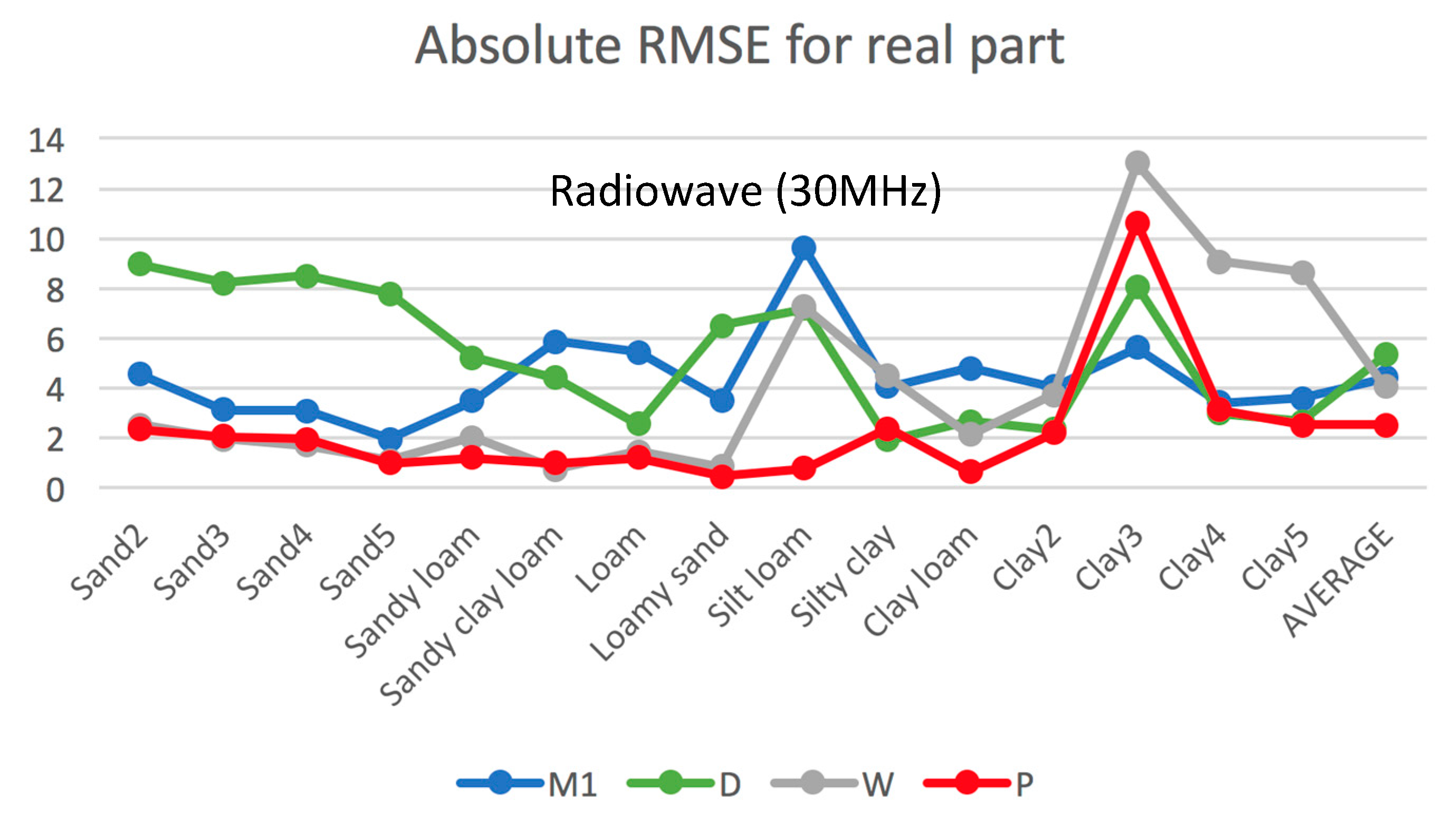
| Soil Texture | Samples | M1 | D | W | P |
|---|---|---|---|---|---|
| Sand2 | L | 4.56 | 8.98 | 2.53 | 2.36 |
| Sand3 | U | 3.13 | 8.23 | 1.95 | 2.06 |
| Sand4 | V | 3.10 | 8.51 | 1.72 | 1.98 |
| Sand5 | W | 1.98 | 7.78 | 1.10 | 0.99 |
| Sandy loam | T | 3.49 | 5.24 | 2.02 | 1.20 |
| Sandy clay loam | Q | 5.86 | 4.41 | 0.77 | 0.99 |
| Loam | N | 5.43 | 2.55 | 1.46 | 1.21 |
| Loamy sand | S | 3.54 | 6.52 | 0.86 | 0.47 |
| Silt loam | P | 9.62 | 7.19 | 7.26 | 0.78 |
| Silty clay | M | 4.07 | 1.94 | 4.49 | 2.38 |
| Clay loam | O | 4.82 | 2.67 | 2.13 | 0.65 |
| Clay2 | J | 4.06 | 2.34 | 3.75 | 2.20 |
| Clay3 | K | 5.63 | 8.07 | 13.00 | 10.63 |
| Clay4 | R | 3.41 | 3.01 | 9.08 | 3.14 |
| Clay5 | X | 3.59 | 2.67 | 8.64 | 2.53 |
| AVERAGE | 4.42 | 5.34 | 4.05 | 2.24 |
© 2017 by the authors. Licensee MDPI, Basel, Switzerland. This article is an open access article distributed under the terms and conditions of the Creative Commons Attribution (CC BY) license (http://creativecommons.org/licenses/by/4.0/).
Share and Cite
Park, C.-H.; Behrendt, A.; LeDrew, E.; Wulfmeyer, V. New Approach for Calculating the Effective Dielectric Constant of the Moist Soil for Microwaves. Remote Sens. 2017, 9, 732. https://doi.org/10.3390/rs9070732
Park C-H, Behrendt A, LeDrew E, Wulfmeyer V. New Approach for Calculating the Effective Dielectric Constant of the Moist Soil for Microwaves. Remote Sensing. 2017; 9(7):732. https://doi.org/10.3390/rs9070732
Chicago/Turabian StylePark, Chang-Hwan, Andreas Behrendt, Ellsworth LeDrew, and Volker Wulfmeyer. 2017. "New Approach for Calculating the Effective Dielectric Constant of the Moist Soil for Microwaves" Remote Sensing 9, no. 7: 732. https://doi.org/10.3390/rs9070732