Characterizing Regional-Scale Combustion Using Satellite Retrievals of CO, NO2 and CO2


1
Department of Civil and Environmental Engineering, Massachusetts Institute of Technology, Cambridge, MA 02139, USA
2
Department of Hydrology and Atmospheric Sciences, University of Arizona, Tucson, AZ 85721, USA
*
Author to whom correspondence should be addressed.
Remote Sens. 2017, 9(7), 744; https://doi.org/10.3390/rs9070744
Submission received: 6 June 2017
/
Revised: 7 July 2017
/
Accepted: 13 July 2017
/
Published: 19 July 2017
(This article belongs to the Special Issue Remote Sensing of Greenhouse Gases)
Abstract
:We present joint analyses of satellite-observed combustion products to examine bulk characteristics of combustion in megacities and fire regions. We use retrievals of CO, NO2 and CO2 from NASA/Terra Measurement of Pollution In The Troposphere, NASA/Aura Ozone Monitoring Instrument, and JAXA Greenhouse Gases Observing Satellite to estimate atmospheric enhancements of these co-emitted species based on their spatiotemporal variability (spread, σ) within 14 regions dominated by combustion emissions. We find that patterns in σXCO/σXCO2 and σXCO/σXNO2 are able to distinguish between combustion types across the globe. These patterns show distinct groupings for biomass burning and the developing/developed status of a region that are not well represented in global emissions inventories. We show here that such multi-species analyses can provide constraints on emission inventories, and be useful in monitoring trends and understanding regional-scale combustion.
1. Introduction
The characteristics and scale of global emissions of pollutants and greenhouse gases into the atmosphere are not currently well understood, particularly for regions where substantial emissions occur due to combustion. These combustion processes lead to locally enhanced emissions and production of CO2, as well as various pollutants and other greenhouse gases, which then impact air quality, climate, and ecosystems [1]. Despite the significant environmental impact, estimates of these emissions from combustion remain uncertain, particularly in remote and rapidly developing regions where combustion processes are poorly characterized due to a lack of detailed information including: fuel type, energy-use, combustion practices, and pollution control strategies [1,2]. This uncertainty is exacerbated by limited observations at the spatiotemporal scales necessary to resolve variations in combustion patterns [3].
Here, we highlight the utility of satellite observations in characterizing combustion over large source regions through a joint analysis of observed products typically used for monitoring air quality [4,5]. We focus this analysis on the substantial local emission sources from biomass burning and large urban regions (megacities). These two sources were selected due to their relative source strength, and because they can be readily observed through analysis of satellite retrievals of atmospheric composition, specifically CO, CO2, and NO2 [6,7,8]. Each of these constituents is emitted concurrently during combustion, and exhibits distinct atmospheric signatures that depend on fuel type, combustion technology/process/practice, and regulatory policies in the region. In a combustion process using a hydrocarbon fuel, both CO and CO2 are produced, depending on the completeness of the combustion. In addition, are produced from the oxidation of nitrogen from the fuel itself and from decomposition of in air at high temperatures [9]. Since combustion processes alter local concentrations of CO, CO2, and NO2, an analysis of their relative abundances and enhancements should provide information regarding local combustion sources, processes, and practices.
Important work has been carried out in recent years toward understanding emissions through analysis of enhancements of chemical species (including isotopes) based on ground [10,11,12,13,14], aircraft [15,16], and satellite observations ([7,17,18,19,20]). However, most of these are focused on either field campaigns for specific megacities (e.g., Los Angeles or Paris [14]), specific regions (e.g., Europe by [20]), or specific ratios between two compounds (e.g., ΔCO/ΔCO2, [17] or ΔNOx/ΔCO2, [7]). For satellite analyses in particular, several multi-species studies have been designed to estimate emissions of air pollutants or surface fluxes of greenhouse gases; yet very few studies have focused on analyzing both from complementary datasets. Reuter et al. [18] used the SCanning Imaging Absorption spectroMeter for Atmospheric CHartographY (Envisat/SCIAMACHY) CO2 and NO2 collocated retrievals to determine associated CO2 and NO2 emissions. Following Berezin et al. [21], who used SCIAMACHY and the Global Ozone Monitoring Experiment (METOP/GOME-2) NO2 to derive fossil-fuel CO2 emissions, Konovalov et al. [19] used the Infrared Atmospheric Sounding Interferometer (METOP/IASI) CO, MODIS Aerosol Optical Depth (AOD) and Fire Radiative Power (FRP) to derive wildfire CO2 emissions. Multi-sensor analyses of ozone from several precursors, including MOPITT CO and OMI NO2 have been carried out by Miyazaki et al. [22] and Inness et al. [23], but both mainly focused on chemical weather related analyses. Additionally, while multi-species inverse modeling studies of pollution sources have made progress using satellite data [24], few studies have directly connected and reconciled with emission inventories through improvements in activity levels and emission factors [25].
In this work, we demonstrate that satellite observations can distinguish differences in combustion source characteristics through analysis of the relative patterns in enhancements of CO and CO2, and NO2 and CO, respectively. Additionally, we show that satellite-observed NO2 and CO can further constrain combustion processes including fire phase and the dominant combustion fuel type in megacities (urban regions with >5 million people). We take advantage of the unique opportunity to study combustion patterns and trends within the nexus of air pollution and carbon cycle science, giving us the ability to draw conclusions relevant to both air quality and climate, particularly for regions with few observations and limited information on local combustion processes.
2. Data and Methods
2.1. Satellite Retrievals and Ancillary Datasets
The main datasets used in this study are summarized in Table 1. Global column-averaged dry air mole fractions of CO2 (XCO2), CO (XCO), and NO2 (XNO2) are taken or derived from GOSAT/ACOS, MOPITT, and OMI/DOMINO Level 2 standard retrieval products, respectively. We focus our analysis on these datasets for the year 2010, which is close to the period used by Silva et al. [17] for their ΔCO2/ΔCO analysis. We use the updated ACOS CO2 retrievals (build 3.3) to take advantage of bias improvements in the newer version. Please refer to Table 1 for references where we highlight the retrieval characteristics of these products and the extent to which they have been validated against other measurements.
To complement our analysis over fire regions, we used MODIS FRP in conjunction with fire emissions from the Global Fire Emission Database (GFEDv3 [34]) to relate phases of the fire (i.e., smoldering or flaming) with observed enhancements of XCO and XNO2. We also used the 0.083° resolution ‘Anthromes’ (Anthropogenic Biomes v1) land cover datasets representing the years 2001–2006 from NASA Socioeconomic Data and Applications Center (SEDAC, [35]) as data filters to locate areas of urban and dense settlements. We compare the satellite-observed results of this study with The Emission Database for Global Atmospheric Research (EDGAR v4.2, [36], 0.1° resolution). Lastly, we used energy-use statistics from the World Bank Development Indicators (WBDI, [37]) as proxies for combustion activity and type, in lieu of sufficient GOSAT XCO2 retrievals over megacities (see Section 3.3).
2.2. Regional Enhancements
We designed this analysis to address several specific aims. First, we identify distinct bulk characteristics of combustion across the globe, comparing results across megacity and biomass burning regions. Then, we include a more in-depth investigation of large-scale biomass burning. Finally, we investigate the satellite-observed relationship between energy use and bulk combustion characteristics across 46 megacities at a much higher resolution using CO and NO2 retrievals. We emphasize the ‘bulk’ nature of our analyses as these satellite column retrievals can only represent combustion signatures at broad spatiotemporal scales [4].
2.2.1. Spatiotemporal Filtering
For the large-scale bulk comparisons involving the biomass burning regions, initial regional selection was based on visual inspection of ‘hotspots’ in trace gas abundance as depicted in the monthly-mean distribution XCO2, XCO, and XNO2. Combustion regions were selected within 4° surrounding the center of these hotspots. Though these regions are rather coarse for the study of individual urban areas, they are consistent with the scale of many of the large biomass burning events and allow for a sufficient number of XCO2 retrievals over all regions. To facilitate comparison across regions, we chose to keep the combustion region size constant. Additionally, the resulting combustion characteristics over these larger regions are consistent with smaller scale analyses [17]. We then selected among all combustion regions exhibiting positive monthly-mean cross correlations between the three chemical species. Our regional selection was directed towards minimizing false positive combustion signatures at the expense of missing several false negative locations and keeping in mind retrieval issues over high latitudes (reduced number of observations, larger relative error, etc.). The combustion regions selected are shown as boxes in the Figure 1, along with annual mean concentrations of the three retrieved species used in this work. They correspond to megacity/urban regions in developed nations (New York, California/Los Angeles, Germany/Rhine Ruhr, Japan/Tokyo), megacity/urban regions in developing nations (China/Beijing, India/New Delhi, Middle East/Tehran, Indonesia, and South Africa) and large-scale biomass burning areas in the tropics (Central Africa, Northern Africa, Amazon, Southeast Asia, and Columbia/Equatorial South America).
For the megacity analysis, we performed high resolution spatial filtering similar to Silva et al. [17]. We applied a land-use/land-cover classification over each megacity with population larger than 5 million in 2010 based on 0.083° resolution ‘anthropogenic biomes’ [38]. We chose this data as our spatial filter instead of population density, as this data enables us to locate areas of urban and dense settlements, which allows for a more tractable definition of the urban extent of megacities. We selected only those retrievals of XCO and XNO2 centered over the urban and dense settlement regions and within the contiguous megacity region. The urban extents from the Anthromes are plotted in Figure 1D, and the megacities are shown as black circles in Figure 1.
To minimize the influence of non-combustion sources (e.g., biogenic CO) and the biospheric sink of CO2, we only use retrievals during winter months (for fossil-fuel combustion) and the fire season (for biomass burning) in this analysis. We used the monthly mean XCO2, XCO, and XNO2 distribution to determine the temporal extent of the winter and fire (three months of the fire season centered on the peak month) periods (see Appendix A for more details). We chose to filter the data for these seasons to further enhance the combustion signature, which otherwise is confounded by other sources. It is important to note that our approach on enhancing the anthropogenic combustion signal represents a best-case scenario of the information content of these retrievals, which in the future should be fully exploited through data assimilation [39]. In particular, augmenting GOSAT with the recent NASA OCO-2 XCO2 products [40] should provide a substantially larger number of data points for megacity analysis at finer scale.
2.2.2. Atmospheric Enhancements
After all data were filtered following the aforementioned criteria, atmospheric enhancements were calculated. We assume that the atmospheric signature of the combustion source behaves like a ‘big smoke stack’ situated within a broader region. We can then model this system as a box treating the species abundance at quasi steady-state. Normally, the average regional atmospheric enhancement () for a given species X is determined as the mean difference between the observed abundance over a polluted environment and a specific background value () that is estimated from spatiotemporal statistics or comparison to ‘clean air’ conditions. If we assume that the data exhibits (or can be transformed to) a Gaussian distribution, and where and are the mean and standard deviation of X across the region and specific period, respectively, then . Under these conditions, the standard deviation in the column data across space and time for a given region is a reasonable measure of enhancement due to regional emissions. In addition, we assume that the ratio of standard deviation between species is proportional to the associated enhancement ratios (). This represents an upper bound as this approach assumes high correlation, , considering the relationship: We note that this assumption is valid only upon careful selection of column retrievals, which we have done through our spatiotemporal filters, ensuring that retrievals are highly correlated on a monthly basis over our select regions. This is not an issue for collocated data used for example by [21] or with the regional enhancement approach by [41]. We use the outlined approach since we are limited globally by the low number of XCO2 retrievals. We note that absolute values of satellite-based ratios represent averaged tropospheric column rather than surface or boundary-layer [5], leading to column values much lower than surface measurements report, particularly for NO2. Additionally, the lifetime of NO2 is low relative to both CO and CO2, which will cause the enhancement of XNO2 to be biased low across the regions relative to the other two chemical species. This is important when interpreting the results of this work in context of other studies.
3. Results and Discussion
3.1. Bulk Characteristics in Combustion Regions
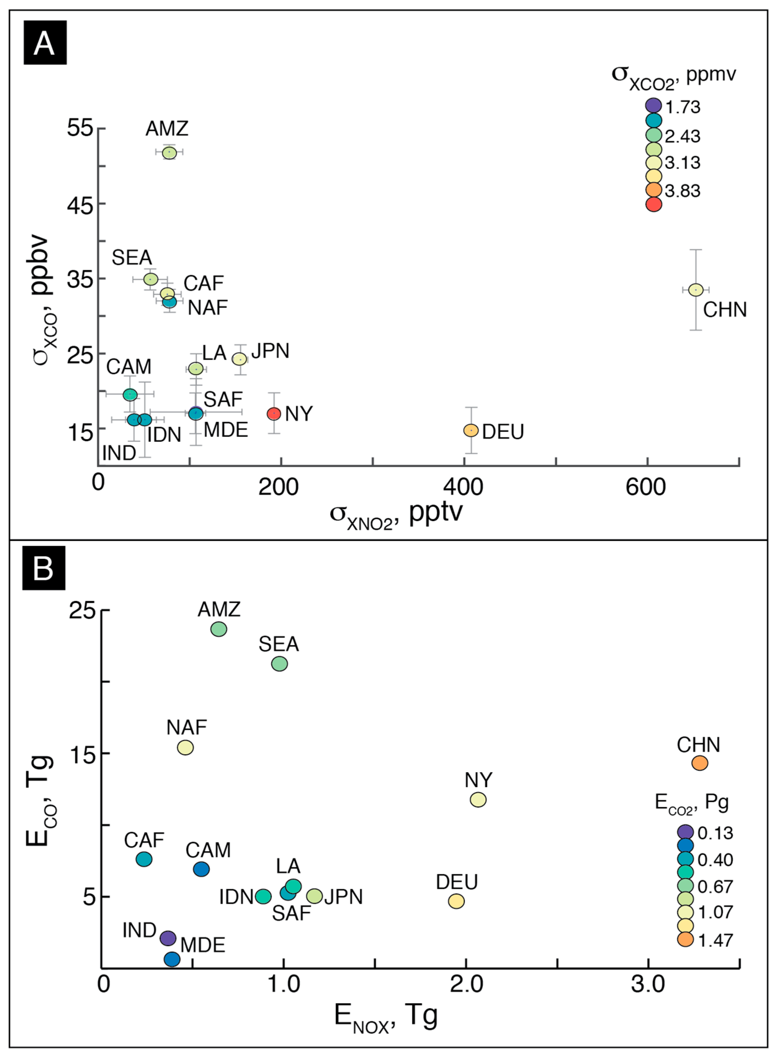
We present in Figure 2A our joint analysis of XCO2, XCO, and XNO2 over selected combustion regions of the world. Figure 2A shows the XCO2 standard deviation (colored circles) plotted as a function of the region’s corresponding XCO and XNO2 standard deviation. We also show in Figure 2A bootstrapped ranges in our estimates accounting for the retrieval precision, and when our assumptions of uniform sampling are relaxed (See Appendix A). This bootstrapping approach was chosen to characterize the uncertainty given the challenges in directly assessing uncertainty given our selection criteria and the relatively small number of XCO2 retrievals. The uncertainty of σXCO2 estimated by this bootstrapping method ranges from 14% to 65% of σXCO2 with the low and high ends corresponding to NY/CHN and SAF/MDE, respectively. LA lies in the median of 25%. Even with these range of estimates, we see a reasonable differentiation between the combustion characteristics (activity and efficiency).
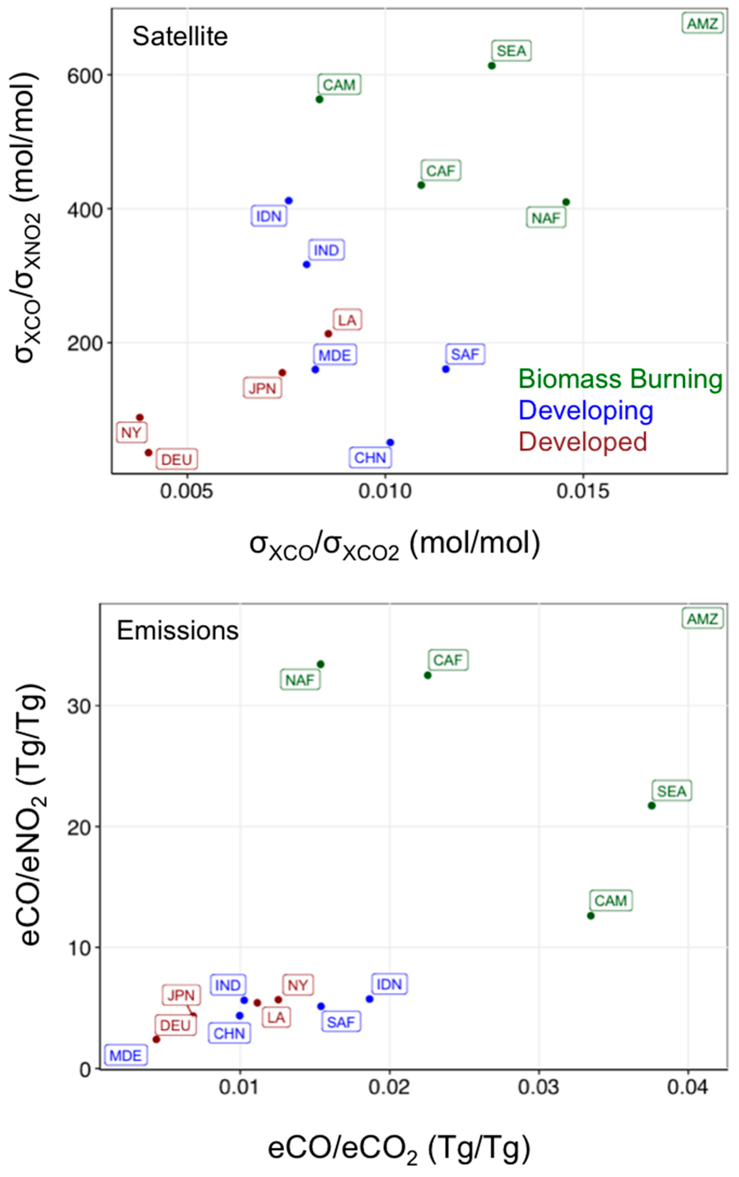
A similar diagram is plotted for an emission-based estimate of combustion patterns. As noted in [10], the emission ratios can be comparable to a concentration-based approach when confounding influences are appropriately considered. We calculated the total emissions of CO, NOx and CO2 across each region, replacing the large-scale biomass burning component in EDGAR with GFEDv.3 and excluding non-road transportation sources. The exclusion of non-road sources will likely lead to a small underestimation of total emissions [42]. The relative distributions between the observations and the emissions inventories are similar, with the biomass burning regions both containing relatively high σ and emissions of CO and low NO2. Both plots also show that the anthropogenic regions have relatively higher σ and emissions of NO2 and lower CO. A more quantitative comparison of the observations and emissions can be completed through the calculation of the CO/CO2 and CO/NO2 ratios. Given that all three constituents are co-emitted during combustion, these ratios can be associated with the bulk combustion characteristics of a given region, as described in Section 2.2. The ratios were calculated from the observed σ and EDGARv4.2 emissions, shown in Figure 3 with colors representing the assumed dominant combustion type.
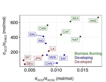
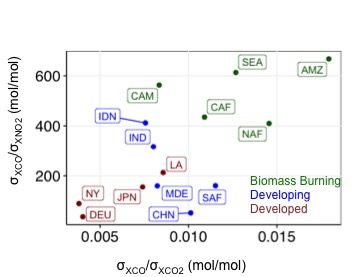
The top panel of Figure 3 shows the observed ratio comparison, where the distinction between the three combustion signatures is apparent. In general, σXCO/σXNO2 responds linearly to σXCO/σXCO2 (r = 0.67), moving from developed through developing to biomass burning regions. Low ratios of both σXCO/σXCO2 and σXCO/σXNO2 correspond to the developed regions, including Germany, New York, and Japan. These results in σXCO/σXCO2 are consistent with previous work by Silva et al. [17], where they found high values of the inverse ratio corresponding to developed regions. This indicates that these developed regions produce relatively small amounts of CO per emitted molecule of CO2, and relatively large amounts of NO2 per emitted molecule of CO. High ratios of σXCO/σXCO2 and σXCO/σXNO2 correspond to the biomass burning regions, which produce relatively more CO to both NO2 and CO2. Developing regions are in between the two, consistent with markedly less efficient combustion than developed regions, but still more efficient than pure biomass burning.
The analogous plot to the observed ratios in Figure 1A for EDGARv4.2 emissions is shown in the bottom panel of Figure 3. Consistent with the satellite-derived ratios, the emissions-based eCO/eCO2 ratio responds linearly to eCO/eNO2 (r = 0.69), and they also show a difference between biomass burning and anthropogenic combustion types. However, there is no distinction between the various developed and developing regions, as exists in the observational distribution. There is little coherence within the anthropogenic regions that could inform this work as to exactly why the emissions inventory is inconsistent with the observations, indicating that both the emission ratios eCO/eCO2 and eCO/eNO2 do not reproduce the observed ratios.
Given that the ratios of emissions and concentrations are different quantities, they cannot be directly compared without the use of a model or some other transfer function. However, it is apparent from Figure 3 that there is an overall relationship between these ratios. We hypothesize that these are related to the dominant combustion characteristics, driven largely by emissions. As a back of the envelope comparison in this work, we normalize both distributions to the highest value in each, the Amazon region. The slope of the line between σXCO/σXCO2 and σXCO/σXNO2 was then calculated for the scaled distributions of both the emission ratios and the observed ratios. The comparison of these two slopes is a useful way to test if the observed distribution of combustion products matches that of the emissions inventories. The slopes match reasonably well, with an observed ratio slope of 0.99 ± 0.32 and an emission ratio slope of 0.80 ± 0.24. Though the slopes agree to within ~20% and their standard errors, the slopes of both distributions are likely dominated by the substantial differences between the anthropogenic and biomass burning regions, a feature captured by both the emissions and the observations. Ultimately, the inconsistencies between the ratios from observations and emissions could be formally reconciled through a data assimilation framework that accounts for all three chemical species observed and related confounding factors.
3.2. Bulk Characteristics in Fire Regions
Analysis of combustion through these three constituents (CO2, CO and NO2) can be useful in the study of fire dynamics and behavior. Due to limited information, most bottom-up emission inventories at present specify the phase of a fire from emission ratios derived from concentration measurements taken near the fire region during specific field campaigns (e.g., [43]). Here, we show that the enhanced atmospheric signal of CO2 from fires can be derived from observations of NO2 and CO. ‘Flaming’ fires are more intense and emit more NO2 (from fuel nitrogen and N2 thermal decomposition at hotter temperatures). They typically show more efficient fire combustion characteristics than the less-intense ‘smoldering’ fires, which occur at relatively colder/wetter conditions and emit significantly more CO [43]. We see evidence supporting this idea from CO and NO2 satellite retrievals, particularly over the Amazon. Daily average time-series of XCO2, XCO, and XNO2 over the Amazon and Southeast Asia are shown in Figure 4A, along with plots of daily GFEDv3 CO emissions and MODIS FRPmax (maximum Fire Radiative Power). The daily GFEDv3 CO emissions were derived from its daily fraction emissions database. A spatial plot over the Amazon (AMZ) during September and over Southeast Asia (SEA) during March is shown in Figure 4B, where the numbers 1 to 3 correspond to the peaks in FRP for both time and space. These months correspond to the respective peak month of the corresponding fire season for these regions. While enhancements of atmospheric CO2 due to fires are not evident due to limited XCO2 retrievals, the spatiotemporal patterns of XCO and XNO2 indicate a dominant bulk flaming phase early in the season (higher NO2 and lower CO) and a smoldering phase later in the season (lower NO2 and higher CO) for year 2010 over AMZ (near Mato Grosso). In SEA (near Cambodia), we see a unimodal distribution in timing and location of the peaks in XCO and XNO2. These patterns correspond well to the spatial and temporal patterns in FRPmax (a measure of fire intensity) over these regions. In AMZ, the first peak in FRP corresponds well with the peak in XNO2 (Figure 4A) and the general location of relatively higher XNO2 shown in Figure 4B. The second peak on the other hand corresponds with the peak in CO (Figure 4A) and the general location of higher CO (Figure 4B). However, the timing of CO emissions from GFEDv3 qualitatively follows more with the 2 peaks in FRP over AMZ. Timing differences between GFED and FRP during the start and end of the main fire events are attributed to errors in our Gaussian fit, which is sensitive to outliers. Nonetheless, we highlight here that while fire activity in newer fire emission inventories is constrained by FRP [44], the fire combustion efficiency could also be constrained by XCO and XNO2. A similar approach using AOD and/or CO has been proposed by Ichoku and Ellison [45] and Konavalov et al. [19]. Most recently, Tang and Arellano [46] demonstrated the utility of jointly analyzing XCO, XNO2, AOD, and FRP retrievals in distinguishing the dominant phase of large fire events in the Amazon. Following Mishra et al. [47] and Schreier et al. [48], they showed that enhancements of XNO2 (XCO and AOD) due to fires are proportional (inversely proportional) to the maximum FRP observed for these events. These relationships are stoichiometrically consistent with flaming and smoldering characteristic of biomass/vegetation combustion. Hence, enhancement ratios of CO (or aerosols) to NO2 (in lieu of CO2) can then be estimated from available satellite retrievals. The joint distribution of FRP and these enhancement ratios can be analogous to looking at the joint phase of fire activity and efficiency. This distribution can potentially provide constraints on emission parameters in fire emission models like GFED. We are currently extending the same analysis by Tang and Arellano [46] to multi-species inversion of emission parameters for the Amazon and other fire regions.
3.3. Bulk Characteristics in Megacities
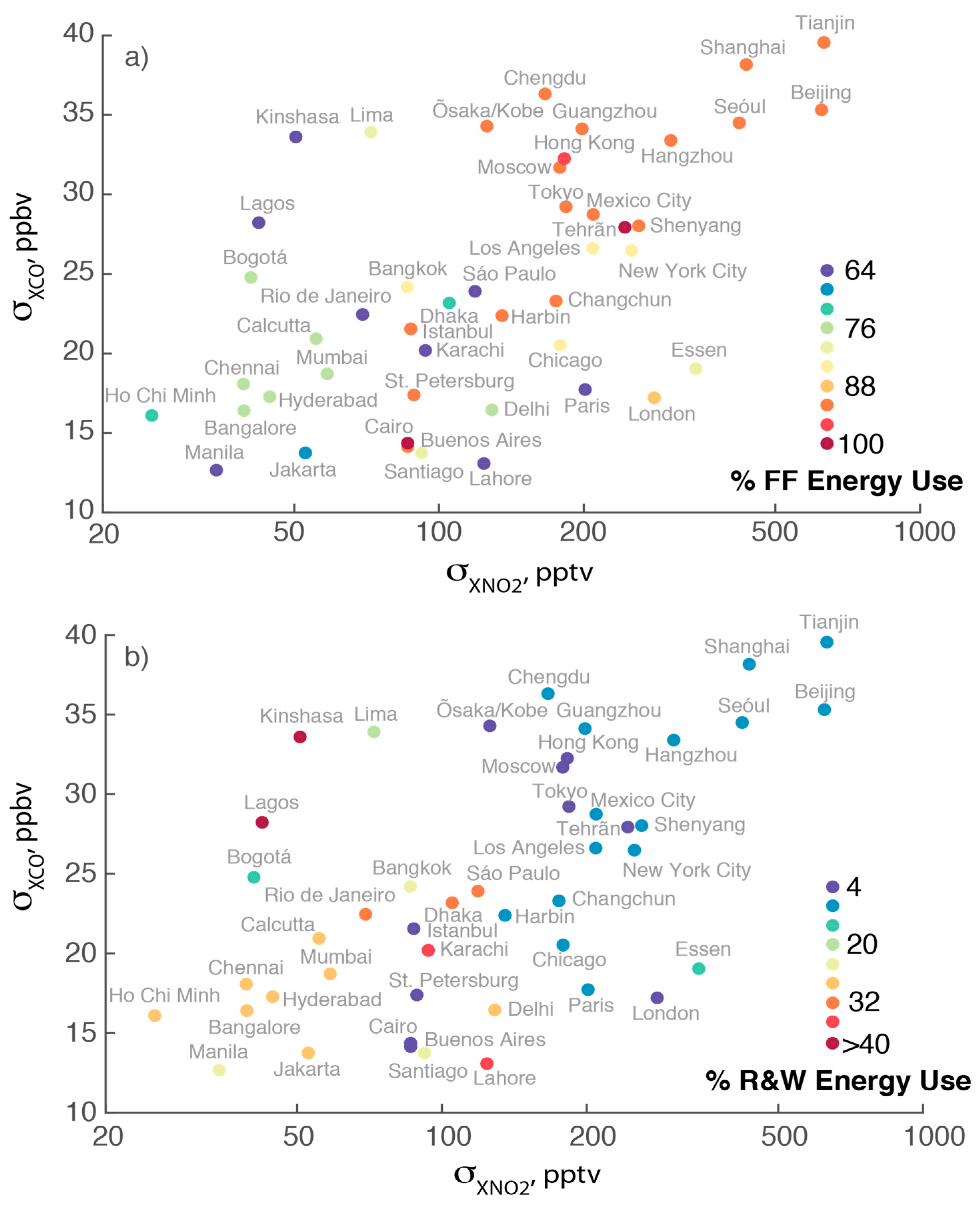
We extend our joint analysis to identify combustion patterns related to energy-use over megacities using World Bank Development Indicators (WBDI) country-based energy-use statistics as proxies for combustion activity, along with the Anthrome dataset for spatial filtering (described in Section 2.2). The WBDI were used because this final analysis over megacities is at too fine a spatial resolution for adequate satellite-based sampling of CO2. The use of coal, oil, and gas for energy and heating is broadly associated with large combustion activity (industries) and high-temperature combustion (power plants), which lend themselves to cost-effective centralized efficiency improvements and pollution control measures [49]. In contrast, the use of biofuel and waste as an energy source for domestic heating and cooking is associated with low-temperature combustion with little or no control technologies in place. In Figure 5, we plot WBDI percent energy consumption by fuel type (fossil-fuel versus combustible renewable and waste) across 46 megacities as a function of XCO and XNO2 spread for the entire year 2010. We show in Figure 5a that most megacities in countries that consume a larger proportion (>75%) of fossil-fuel for energy (i.e., US, China, Japan, Germany, UK), show higher CO and NO2 enhancements than megacities using a higher proportion (>15%) of waste fuels (i.e., India, Brazil, Bangladesh) (see Figure 5b). There are several exceptions to this, most notably Paris, France. In France, nuclear energy is common, so percent waste and fossil-fuel energy consumption are poor metrics for the assessment of combustion processes, and instead the mixture of CO and NO2 measured over this region is more related to transportation and other sectors. Such patterns imply differences in local combustion activity and/or efficiency, and consequently emissions [50], which cannot be completely disentangled through an analysis of XCO and XNO2 alone. However, the patterns that we see are broadly in agreement with CO/NOX molar ratios from the WMO Megacity report [1] showing higher ratios in Sao Paulo, Santiago, Buenos Aires, and Mexico City than the ratios observed in most US cities and Paris in recent decades. A similar agreement in our current understanding of main energy-use and combustion patterns (e.g., EDGAR) can be seen in Los Angeles, Beijing, Tehran, and Dhaka, which all show distinct differences in energy use and the satellite-observed distributions that are related to differences in local emission processes. However, it is difficult at present to compare these values with ground- and aircraft-based enhancement ratios due to the varying scales and representativeness issues [12,16].
Nevertheless, the relationships between relatively frequent measurements of CO and NO2 with energy-use could potentially be leveraged in ways that yield a more complete process-based understanding of CO2 emissions across poorly observed regions. For example, due to issues related to retrieval error and cloud cover, there are no available satellite retrievals of CO2 in 2010 over Kinshasa, a city of 9 million people in the Democratic Republic of Congo. Information regarding CO, NO2, and energy use could be combined to infer the efficacy of pollution control and energy efficiency measures, diagnose the energy mix in different regions, and improve constraint on regional CO2 emissions.
4. Summary and Implications
This work presents a proof-of-concept on observational constraints from current satellite retrievals on bulk characteristics of combustion over megacities and fire regions. We took the approach of estimating CO, NO2, and CO2 enhancements based on their spatiotemporal variability and examined the relative patterns in their joint distribution. We find distinct patterns in bulk characteristics across regions with clear fire or fossil fuel combustion signatures from jointly analyzing GOSAT/ACOS CO2, MOPITT CO, and OMI NO2, retrievals. While promising, our results using these three retrievals are limited to characterizing broad regions due to coarse spatial filtering required for an adequate number of GOSAT CO2 retrievals. Additionally, we show that satellite observations of NO2 and CO can provide useful constraints on fire behavior and dynamics; and we use energy-use statistics to further examine megacity-scale combustion, where we find higher and in megacities using more fossil fuel than waste fuel.
Our results show the utility of this approach for emissions monitoring, verifying and reporting (MRV), process understanding of combustion in current and emerging megacities, and for potentially characterizing anthropogenic CO2 sources. The addition of both CO and NO2 to a space-based analysis of CO2 allows for a more complete and consistent characterization of regional combustion. Analysis of their joint distributions has considerable potential utility in future integrated constituent data assimilation activities where collocation and estimating atmospheric enhancements can be better addressed. This is especially the case with additional data from the OCO-2 mission. Furthermore, such multi-platform/multi-sensor analysis of various chemical species may be used to understand industrial development [2]. This work motivates the need for continuous and preferably collocated satellite measurements of atmospheric composition, including CH4 [51], and studies related to improving the applicability and integration of these observations with ground- and aircraft- based measurements (e.g., DISCOVER-AQ, [52]).
Appendix A
A.1. Bootstrapping Methodology
These estimates are calculated from a Monte Carlo (bootstrap) approach, which we outlined as follows: first, we drew 1000 samples from normally-distributed retrieval—i.e., where is the retrieval value and is its reported precision; then, we calculated the enhancement as the spread of a randomly-selected subset of the data for each sample (20% of data are denied both across the region and time period); and lastly, we calculated the spread of these enhancements across all samples and report this as our range (represented as light line bars in Figure 1A).
A.2. Time Periods and Selection Regions
The ultimate goal of the selection criteria was to capture regions with elevated concentrations of CO, NO2, or CO2, where those enhancements were likely related to combustion. Regions were selected based on visual inspection of hotspots in the satellite observations of CO, NO2, and CO2, in regions that had positive correlations in the enhancements of all three species.
The months (January–December as 1–12) that passed the selection criteria for each region are listed below. Megacity/urban combustion regions are generally during the local winter period (particularly for midlatitude regions) while for biomass burning it is dependent on fire season.
NY = [12,1,2,3]
DEU = [12,1,2,3]
LA = [12,1,2,3]
SEA = [12,1,2,3]
CAF = [6,7,8]
NAF = [12,1,2]
AMZ = [8,9,10]
SAF = [6,7,8]
CAM = [2,3,4]
JPN = [12,1,2,3]
MDE = [12,1,2,3]
IDN = [9,10,11]
IND = [3,4,5]
CHN = [12,1,2,3]
Acknowledgments
This work is supported by NASA ACMAP Grant NNX13AK24G. We acknowledge MOPITT, OMI, MODIS/FIRMS/LANCE, GOSAT/ACOS, GFED and EDGAR teams for data on CO, NO2, FRP, CO2, and associated emissions, respectively. We also thank Kevin Bowman, the NASA CMS team, and Wenfu Tang for helpful insights.
Author Contributions
S.J.S. and A.F.A. conceived and designed the experiments; S.J.S. and A.F.A. analyzed the data; S.J.S. and A.F.A. wrote the paper.
Conflicts of Interest
The authors declare no conflict of interest.
References
- Zhu, T.; Melamed, M.; Parrish, D.; Gauss, M.; Klenner, L.G.; Lawrence, M.; Konare, A.; Liousse, C. WMO/IGAC Impacts of Megacities on Air Pollution and Climate. Available online: http://www.wmo.int/pages/prog/arep/gaw/documents/GAW_205_DRAFT_13_SEPT.pdf (accessed on 6 June 2017).
- Creutzig, F.; Baiocchi, G.; Bierkandt, R.; Pichler, P.P.; Seto, K.C. Global typology of urban energy-use and potentials for an urbanization mitigation wedge. Proc. Natl. Acad. Sci. USA 2015, 112, 6283–6288. [Google Scholar] [CrossRef] [PubMed]
- Hutyra, L.R.; Duren, R.; Gurney, K.R.; Grimm, N.; Kort, E.A.; Larson, E.; Shrestha, G. Urbanization and the carbon cycle: Current capabilities and research outlook from the natural sciences perspective. Earth’s Future 2014, 10, 473–495. [Google Scholar] [CrossRef]
- Duncan, B.N.; Prados, A.I.; Lamsal, L.N.; Liu, Y.; Streets, D.G.; Gupta, P.; Hilsenrath, E.K.; Ralph, A.; Nielsen, J.E.; Beyersdorf, A.J.; et al. Satellite data of atmospheric pollution for US air quality applications: Examples of applications, summary of data end-user resources, answers to FAQs, and common mistakes to avoid. Atmos. Environ. 2014, 94, 647–662. [Google Scholar] [CrossRef]
- Martin, R.V. Satellite remote sensing of surface air quality. Atmos. Environ. 2008, 42, 7823–7843. [Google Scholar] [CrossRef]
- Pommier, M.; Mclinden, C.A.; Deeter, M. Relative changes in CO emissions over megacities based on observations from space. Geophys. Res. Lett. 2013, 40, 3766–3771. [Google Scholar] [CrossRef] [Green Version]
- Hakkarainen, J.; Ialongo, I.; Tamminen, J. Direct space-based observations of anthropogenic CO2 emission areas from OCO-2. Geophys. Res. Lett. 2016, 43. [Google Scholar] [CrossRef]
- Duncan, B.N.; Lamsal, L.N.; Thompson, A.M.; Yoshida, Y.; Lu, Z.; Streets, D.G.; Pickering, K.E. A space-based, high-resolution view of notable changes in urban NOx pollution around the world (2005–2014). J. Geophys. Res. Atmos. 2016, 121, 976–996. [Google Scholar] [CrossRef]
- Flagan, R.C.; Seinfeld, J.H. Fundamentals of Air Pollution Engineering; Courier Corporation: Mineola, NY, USA, 2013. [Google Scholar]
- Parrish, D.D.; Kuster, W.C.; Shao, M.; Yokouchi, Y.; Kondo, Y.; Goldan, P.D.; Shirai, T. Comparison of air pollutant emissions among Mega-Cities. Atmos. Environ. 2009, 43, 6435–6441. [Google Scholar] [CrossRef]
- Pollack, I.B.; Ryerson, T.B.; Trainer, M.; Neuman, J.A.; Roberts, J.M.; Parrish, D.D. Trends in ozone, its precursors, and related secondary oxidation products in Los Angeles, California: A synthesis of measurements from 1960 to 2010. J. Geophys. Res. 2013, 118, 5893–5911. [Google Scholar] [CrossRef]
- Lopez, M.; Schmidt, M.; Delmotte, M.; Colomb, A.; Gros, V.; Janssen, C. CO, NOX and 13CO2 as tracers for fossil fuel CO2: Results from a pilot study in Paris during winter 2010. Atmos. Chem. Phys. 2013, 13, 7343–7358. [Google Scholar] [CrossRef]
- Lindenmaier, R.; Dubey, M.K.; Henderson, B.G.; Butterfield, Z.T.; Herman, J.R.; Rahn, T.; Lee, S.-H. Multi-scale observations of CO2, 13CO2, and pollutants at Four Corners for emission verification and attribution. Proc. Natl. Acad. Sci. USA 2014, 111, 8386–8391. [Google Scholar] [CrossRef] [PubMed]
- Hassler, B.; McDonald, B.C.; Frost, G.J.; Borbon, A.; Carslaw, D.C.; Civerolo, K.; Pollack, I.B. Analysis of long-term observations of NOx and CO in megacities and application to constraining emissions inventories. Geophys. Res. Lett. 2016, 43, 9920–9930. [Google Scholar] [CrossRef]
- Turnbull, J.C.; Karion, A.; Fischer, M.L.; Faloona, I.; Guilderson, T.; Lehman, S.J.; Miller, B.R.; Miller, J.B.; Montzka, S.; Sherwood, T.; et al. Assessment of fossil fuel carbon dioxide and other anthropogenic trace gas emissions from airborne measurements over Sacramento, California in spring 2009. Atmos. Chem. Phys. 2011, 11, 705–721. [Google Scholar] [CrossRef] [Green Version]
- Brioude, J.; Angevine, W.M.; Ahmadov, R.; Kim, S.W.; Evan, S.; McKeen, S.A.; Hsie, E.Y.; Frost, G.J.; Neuman, J.A.; Pollack, I.B.; et al. Top-down estimate of surface flux in the Los Angeles Basin using a mesoscale inverse modeling technique: Assessing anthropogenic emissions of CO, NOx and CO2 and their impacts. Atmos. Chem. Phys. 2013, 13, 3661–3677. [Google Scholar] [CrossRef]
- Silva, S.J.; Arellano, A.F.; Worden, H. Toward anthropogenic combustion emission constraints from space-based analysis of urban CO2/CO sensitivity. Geophys. Res. Lett. 2013, 40, 4971–4976. [Google Scholar] [CrossRef]
- Reuter, M.; Ryerson, T.B.; Trainer, M.; Neuman, J.A.; Roberts, J.M.; Parrish, D.D. Decreasing emissions of NOx relative to CO2 in East Asia inferred from satellite observations. Nat. Geosci. 2014, 7, 792–795. [Google Scholar] [CrossRef]
- Konovalov, I.B.; Berezin, E.V.; Ciais, P.; Broquet, G.; Beekmann, M.; Hadji-Lazaro, J.; Clerbaux, C.; Andreae, M.O.; Kaiser, J.W.; Schulze, E.D.; et al. Constraining CO2 emissions from open biomass burning by satellite observations of co-emitted species: A method and its application to wildfires in Siberia. Atmos. Chem. Phys. 2014, 14, 10383–10410. [Google Scholar] [CrossRef] [Green Version]
- Konovalov, I.B.; Berezin, E.V.; Ciais, P.; Broquet, G.; Zhuravlev, R.V.; Janssens-Maenhout, G. Estimation of fossil-fuel CO2 emissions using satellite measurements of ‘proxy’ species. Atmos. Chem. Phys. 2016, 16, 13509–13540. [Google Scholar] [CrossRef]
- Berezin, E.V.; Konovalov, I.B.; Ciais, P.; Richter, A.; Tao, S.; Janssens-Maenhout, G.; Beekmann, M.; Schulze, E.-D. Multiannual changes of CO2 emissions in China: Indirect estimates derived from satellite measurements of tropospheric NO2 columns. Atmos. Chem. Phys. 2013, 13, 255–309. [Google Scholar] [CrossRef]
- Miyazaki, K.; Eskes, H.J.; Sudo, K. A tropospheric chemistry reanalysis for the years 2005–2012 based on an assimilation of OMI, MLS, TES and MOPITT satellite data. Atmos. Chem. Phys. 2015, 15, 8315–8348. [Google Scholar] [CrossRef]
- Inness, A.; Blechschmidt, A.M.; Bouarar, I.; Chabrillat, S.; Crepulja, M.; Engelen, R.J.; Eskes, H.; Flemming, J.; Gaudel, A.; Hendrick, F.; et al. Data assimilation of satellite retrieved ozone, carbon monoxide and nitrogen dioxide with ECMWF’s Composition-IFS. Atmos. Chem. Phys. 2015, 15, 5275–5303. [Google Scholar] [CrossRef]
- Fortems-Cheiney, A.; Chevallier, F.; Pison, I.; Bousquet, P.; Saunois, M.; Szopa, S.; Cressot, C.; Kurosu, T.P.; Chance, K.; Fried, A. The formaldehyde budget as seen by a global-scale multi-constraint and multi-species inversion system. Atmos. Chem. Phys. 2012, 12, 6699–6721. [Google Scholar] [CrossRef]
- Streets, D.G.; Timothy, C.; Gregory, R.C.; Benjamin, F.; Russell, R.D.; Bryan, N.D.; David, P.E.; John, A.H.; Daven, K.H.; Marc, R.H.; Daniel, J.J.; et al. Emissions estimation from satellite retrievals: A review of current capability. Atmos. Environ. 2013, 77, 1011–1042. [Google Scholar] [CrossRef]
- Measurements of Pollution in the Troposphere (MOPITT). Available online: https://www2.acom.ucar.edu/mopitt (accessed on 6 June 2017).
- Deeter, M.N.; Martínez-Alonso, S.; Edwards, D.P.; Emmons, L.K.; Gille, J.C.; Worden, H.M.; Pittman, J.V.; Daube, B.C.; Wofsy, S.C. Validation of MOPITT Version 5 Thermal-Infrared, near-infrared, and multispectral carbon monoxide profile retrievals for 2000–2011. J. Geophys. Res. 2013. [Google Scholar] [CrossRef]
- TEMIS–Tropospheric NO2. Available online: http://www.temis.nl/airpollution/no2.html (accessed on 6 June 2017).
- Boersma, K.F.; Jacob, D.J.; Bucsela, E.J.; Perring, A.E.; Dirksen, R.; van der A, R.J.; Yantosca, R.M.; Park, R.J.; Wenig, M.O.; Bertram, T.H.; et al. Validation of OMI tropospheric NO2 observations during INTEX-B and application to constrain NOX emissions over the eastern United States and Mexico. Atmos. Environ. 2008, 42, 4480–4497. [Google Scholar] [CrossRef] [Green Version]
- GOSAT Project. Available online: www.gosat.nies.go.jp (accessed on 6 June 2017).
- Crisp, D.; Frankenberg, C.; Messerschmidt, J.; Wennberg, P.O.; Wunch, D.; Yung, Y.L. The ACOS CO2 retrieval algorithm—Part II: Global XCO2 data characterization. Atmos. Meas. Tech. 2012, 5, 687–707. [Google Scholar] [CrossRef]
- Fire Information for Resource Management System. Available online: firms.modaps.eosdis.nasa.gov (accessed on 6 June 2017).
- Freeborn, P.H.; Wooster, M.J.; Roy, D.P.; Cochrane, M.A. Quantification of MODIS fire radiative power (FRP) measurement uncertainty for use in satellite-based active fire characterization and biomass burning estimation. Geophys. Res. Lett. 2014, 41, 1988–1994. [Google Scholar] [CrossRef]
- Global Fire Emissions Database. Available online: http://www.globalfiredata.org (accessed on 6 June 2017).
- Socioeconomic Data and Applications Center. Available online: http://sedac.ciesin.columbia.edu (accessed on 6 June 2017).
- EDGAR. Available online: http://edgar.jrc.ec.europa.eu (accessed on 6 June 2017).
- World Bank Open Data. Available online: http://data.worldbank.org (accessed on 6 June 2017).
- Ellis, E.C.; Ramankutty, N. Putting people in the map: Anthropogenic biomes of the world. Front. Ecol. Environ. 2008, 6, 439–447. [Google Scholar] [CrossRef]
- Bocquet, M.; Elbern, H.; Eskes, H.; Hirtl, M.; Zöabkar, R.; Carmichael, R.; Flemming, J.; Inness, A.; Pagowski, M.; et al. Data assimilation in atmospheric chemistry models: Current status and future prospects for coupled chemistry meteorology models. Atmos. Chem. Phys. 2015, 15, 5325–5358. [Google Scholar] [CrossRef]
- Orbiting Carbon Observatory. Available online: http://oco.jpl.nasa.gov (accessed on 6 June 2017).
- Kort, E.A.; Frankenberg, C.; Miller, C.E.; Oda, T. Space-based observations of megacity carbon dioxide. Geophys. Res. Lett. 2012, 39. [Google Scholar] [CrossRef]
- Fuglestvedt, J.; Berntsen, T.; Myhre, G.; Rypdal, K.; Skeie, R.B. Climate forcing from the transport sectors. Proc. Natl. Acad. Sci. USA 2008, 105, 454–458. [Google Scholar] [CrossRef] [PubMed]
- Andreae, M.O.; Merlet, P. Emission of trace gases and aerosols from biomass burning. Glob. Biogeochem. Cycles 2001, 15, 955–995. [Google Scholar] [CrossRef]
- Kaiser, J.W.; Heil, A.; Andreae, M.O.; Benedetti, A.; Chubarova, N.; Jones, L.; Morcrette, J.J.; Razinger, M.; Schultz, M.G.; Suttie, M.; et al. Biomass burning emissions estimated with a global fire assimilation system based on observed fire radiative power. Biogeosciences 2012, 9, 527–554. [Google Scholar] [CrossRef] [Green Version]
- Ichoku, C.; Ellison, L. Global top-down smoke-aerosol emissions estimation using satellite fire radiative power measurements. Atmos. Chem. Phys. 2014, 14, 6643–6667. [Google Scholar] [CrossRef] [Green Version]
- Tang, W.; Arellano, A.F., Jr. Investigating dominant characteristics of fires across the Amazon during 2005–2014 through satellite data synthesis of combustion signatures. J. Geophys. Res. Atmos. 2017, 121. [Google Scholar] [CrossRef]
- Mishra, A.K.; Lehahn, Y.; Rudich, Y.; Koren, I. Co-variability of smoke and fire in the Amazon Basin. Atmos. Environ. 2015, 109, 97–104. [Google Scholar] [CrossRef]
- Schreier, S.F.; Richter, A.; Kaiser, J.W.; Burrows, J.P. The empirical relationship between satellite-derived tropospheric NO2 and fire radiative power and possible implications for fire emission rates of NOx. Atmos. Chem. Phys. 2014, 14, 2447–2466. [Google Scholar] [CrossRef]
- Ashford, N.A.; Caldart, C.C. Environmental Law, Policy, and Economics: Reclaiming the Environmental Agenda; MIT Press: Cambridge, MA, USA, 2008. [Google Scholar]
- Liu, Z.; Guan, D.; Wei, W.; Davis, S.J.; Ciais, P.; Bai, J.; Peng, S.; Zhang, Q.; Hubacek, K.; Marland, G.; et al. Reduced carbon emission estimates from fossil fuel combustion and cement production in China. Nature 2015, 524, 335–338. [Google Scholar] [CrossRef] [PubMed]
- Wecht, K.J.; Jacob, D.J.; Sulprizio, M.P.; Santoni, G.W.; Wofsy, S.C.; Parker, R.; Bösch, H.; Worden, J. Spatially resolving methane emissions in California: Constraints from the CalNex aircraft campaign and from present (GOSAT, TES) and future (TROPOMI, Geostationary) satellite observations. Atmos. Chem. Phys. 2014, 14, 8173–8184. [Google Scholar] [CrossRef] [Green Version]
- DISCOVER-AQ Program Home. Available online: http://discover-aq.larc.nasa.gov (accessed on 6 June 2017).
Figure 1.
Annual mean retrieved concentrations of XCO2 (A), XCO (B), and XNO2 (C) for the year 2010 used in this work. Panel (D) shows the urban extents as defined by the Anthromes dataset. Megacity locations are shown as black points, and the boxes represent the combustion regions selected for this analysis.
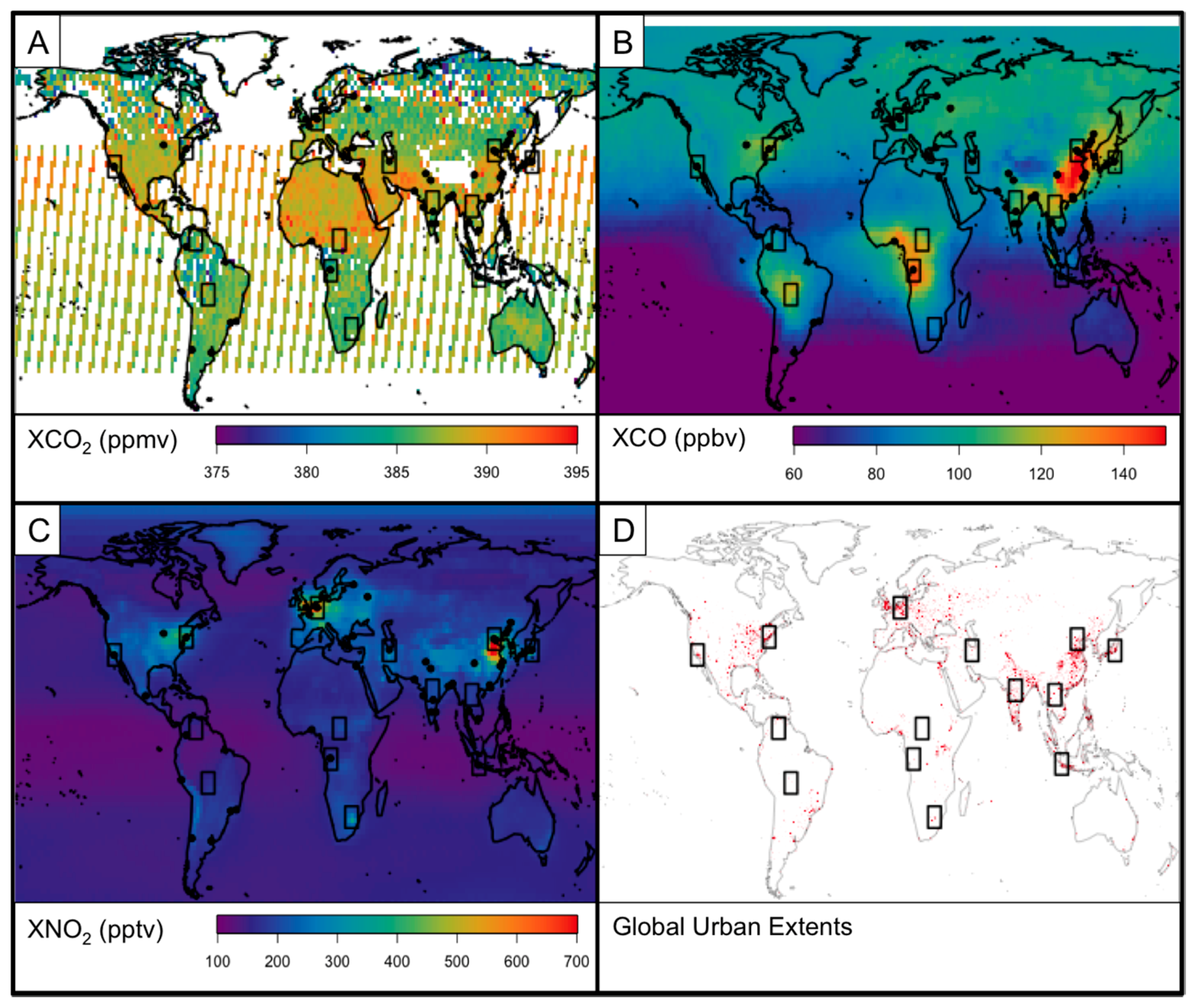
Figure 2.
Regional-scale combustion signatures derived from: (A) spread of XCO2, XCO and XNO2 satellite retrievals, and (B) emission estimates from EDGAR4.2 database with GFEDv3 fire emissions. Note that (A) and (B) have different units. Light line bars correspond to the range of our estimates in (see text for error calculation using boot-strap method).

Figure 3.
Ratios of CO/CO2 plotted against the CO/NO2 ratio, derived from the satellite retrievals (top), and the EDGARv4.2 emissions inventory (bottom). The colors represent the dominant combustion category of a given region.
Figure 3.
Ratios of CO/CO2 plotted against the CO/NO2 ratio, derived from the satellite retrievals (top), and the EDGARv4.2 emissions inventory (bottom). The colors represent the dominant combustion category of a given region.

Figure 4.
Temporal (A) and spatial (B) pattern of large-scale biomass burning signatures (XCO, XNO2, XCO2) over the southern Amazon and Southeast Asia for year 2010 fire season (lines correspond to two-term Gaussian model fits). Estimates of CO emissions (in Tg) from GFEDv3 and retrievals of FRP from MODIS (in GW) are plotted for comparison. Numbers 1 to 3 correspond to the peaks in FRP for both time and space.
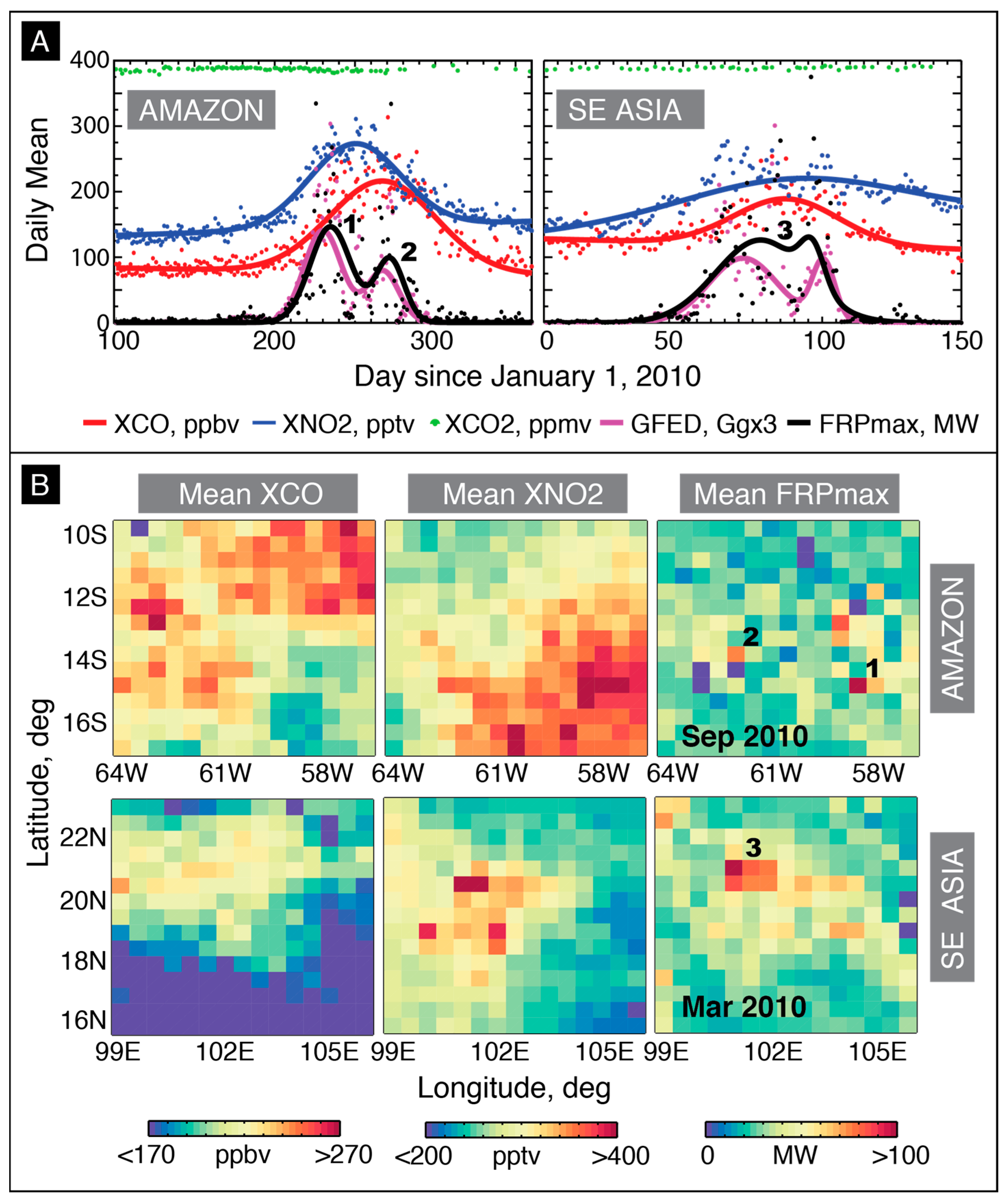
Figure 5.
WBDI percent fossil-fuel energy use versus combustible (a) and renewable and waste consumption (b) across 46 megacities as a function of XCO and XNO2 spread for the year 2010.
Figure 5.
WBDI percent fossil-fuel energy use versus combustible (a) and renewable and waste consumption (b) across 46 megacities as a function of XCO and XNO2 spread for the year 2010.


Table 1.
Satellite data products used in this work.
| Satellite Instrument and Retrieval | Sampling Characteristics | Retrieval Data Characteristics |
|---|---|---|
| (Spectral Region, Resolution, Repeat Cycle, Overpass Time) | (Available Period, Website, Uncertainty, References) | |
| NASA Terra, Measurement of Pollution In The Troposphere (MOPITT v5J), CO total column | TIR/NIR, 22 km, 16 days, 10:30 a.m. | 2000–today, [26], 6–8%, [27] and references therein |
| NASA Aura, Ozone Monitoring Instrument (OMI v2 DOMINO), NO2 trop. column | UV/VIS, 13–26 km, 16 days, 1:45 p.m. | 2004–today, [28], 0.5–1.5e15 molec/cm2, [29] and references therein |
| JAXA GOSAT, Thermal And Near-infrared Sensor for carbon Observation (TANSO-FTS, NASA ACOS b3.3), CO2 column | SWIR, 10.5 km, 3 days, 12:49 p.m. | 2009–today, [30], 1–1.5 ppm, [31] and references therein |
| NASA Terra/Aqua, Moderate Resolution Imaging Spectrometer (MODIS FIRMS MCD14ML c5), FRP | TIR, 1 km, 16 days, 10:30 a.m./1:30 p.m. | 2000/2002–today, [32], 26.6%, [33] and references therein |
© 2017 by the authors. Licensee MDPI, Basel, Switzerland. This article is an open access article distributed under the terms and conditions of the Creative Commons Attribution (CC BY) license (http://creativecommons.org/licenses/by/4.0/).
Share and Cite
MDPI and ACS Style
Silva, S.J.; Arellano, A.F. Characterizing Regional-Scale Combustion Using Satellite Retrievals of CO, NO2 and CO2. Remote Sens. 2017, 9, 744. https://doi.org/10.3390/rs9070744
AMA Style
Silva SJ, Arellano AF. Characterizing Regional-Scale Combustion Using Satellite Retrievals of CO, NO2 and CO2. Remote Sensing. 2017; 9(7):744. https://doi.org/10.3390/rs9070744
Chicago/Turabian StyleSilva, Sam J., and A. F. Arellano. 2017. "Characterizing Regional-Scale Combustion Using Satellite Retrievals of CO, NO2 and CO2" Remote Sensing 9, no. 7: 744. https://doi.org/10.3390/rs9070744
Note that from the first issue of 2016, this journal uses article numbers instead of page numbers. See further details here.