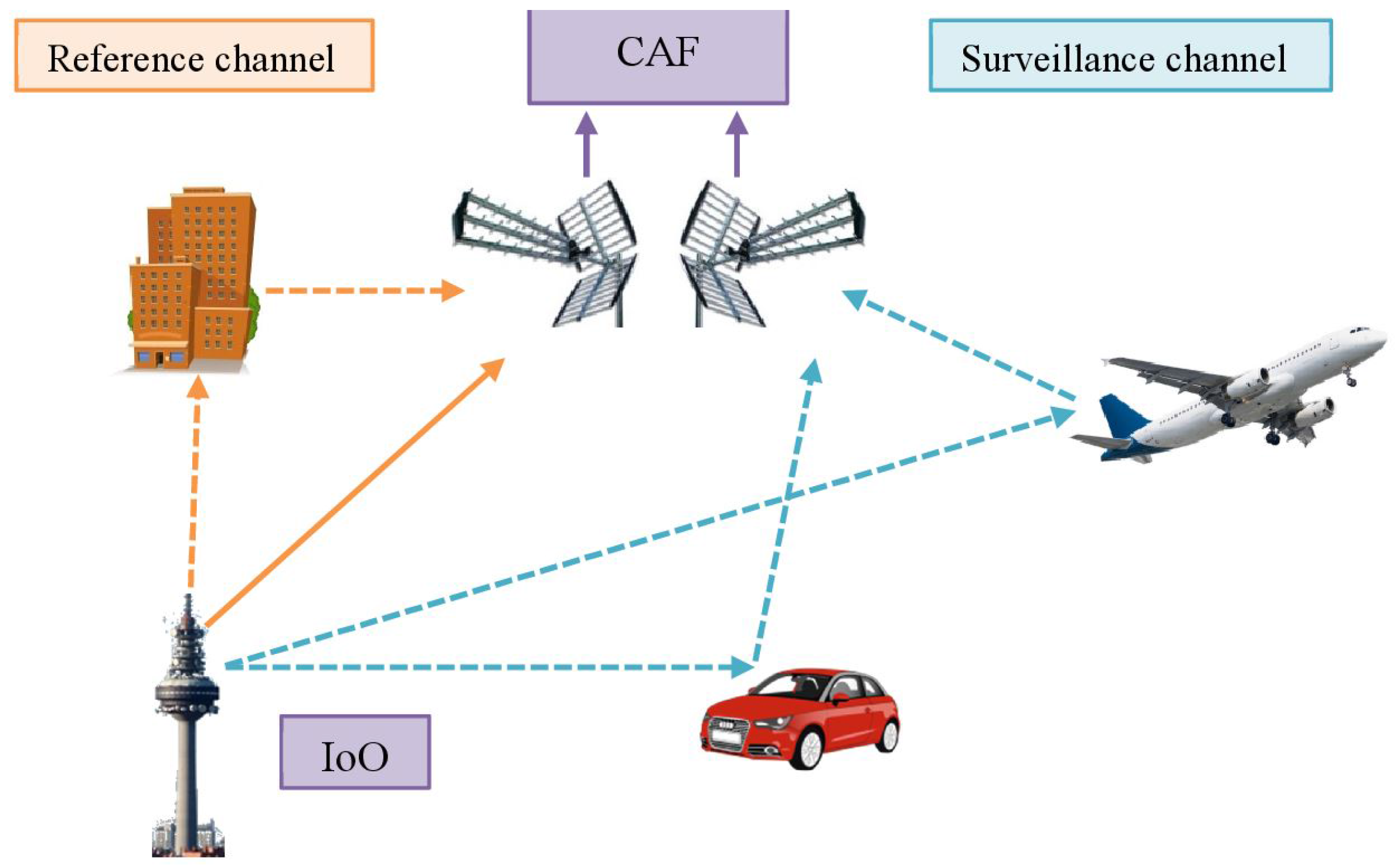
Figure 1.
Basic operating scheme of a Passive Radar System (PRS).
Figure 1.
Basic operating scheme of a Passive Radar System (PRS).
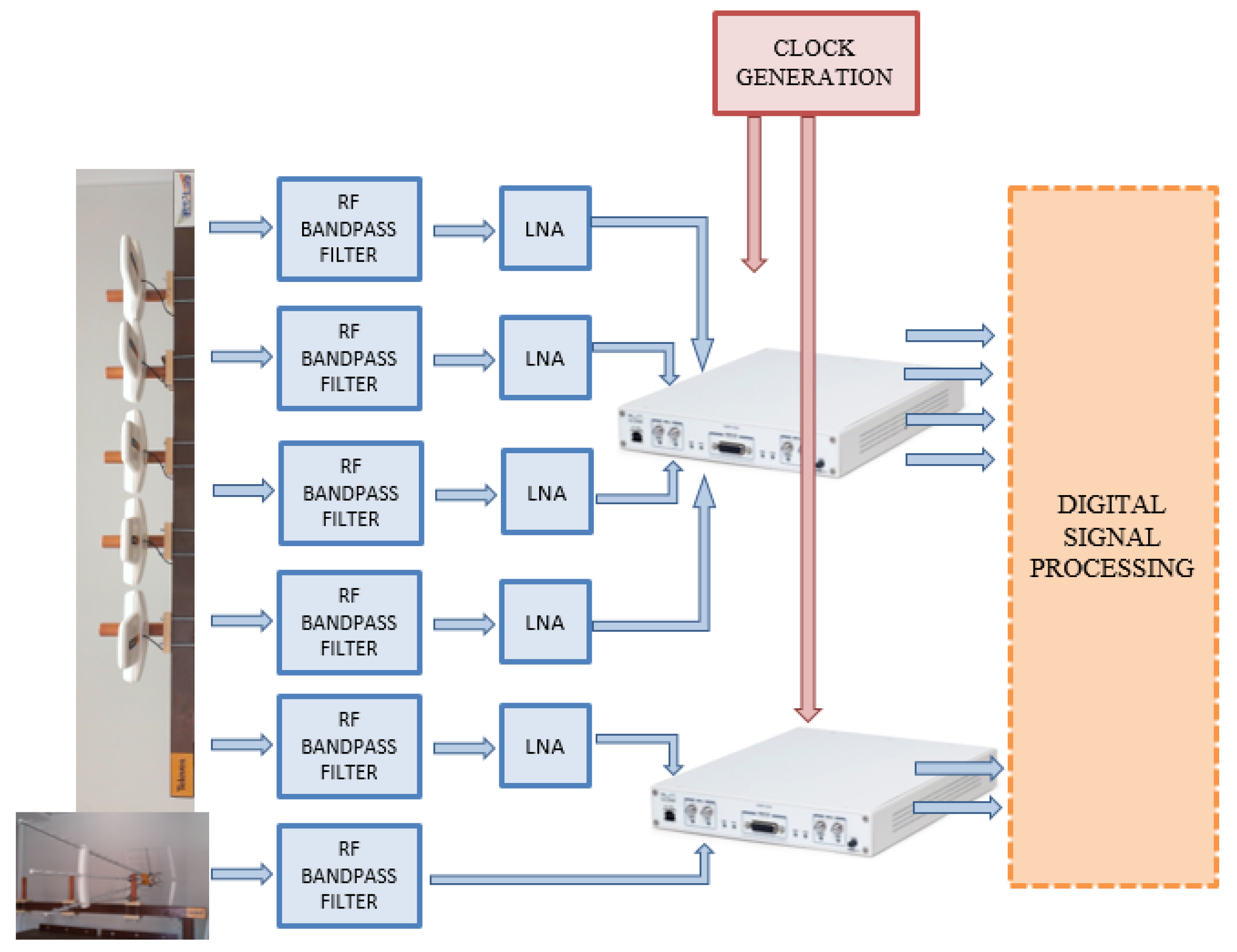
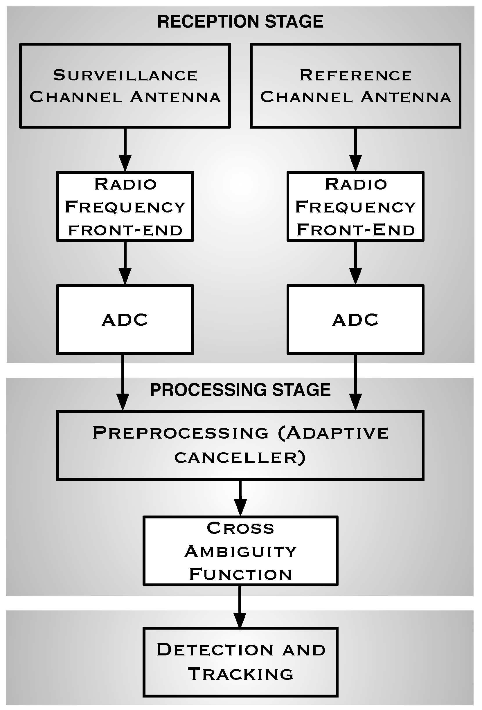
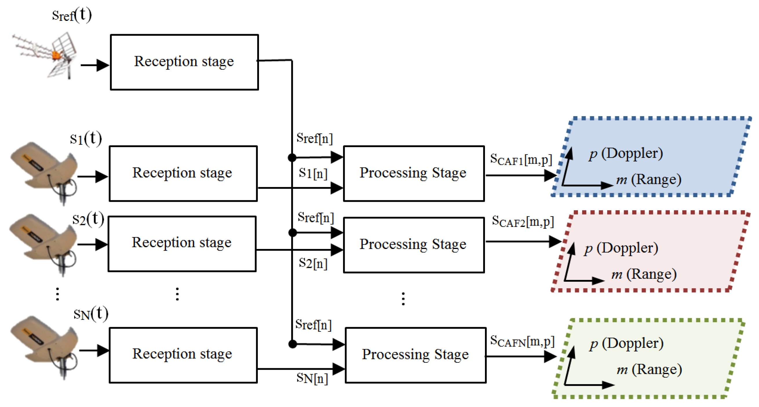
Figure 2.
Basic architecture of a PRS with one surveillance channel and one reference channel.
Figure 2.
Basic architecture of a PRS with one surveillance channel and one reference channel.
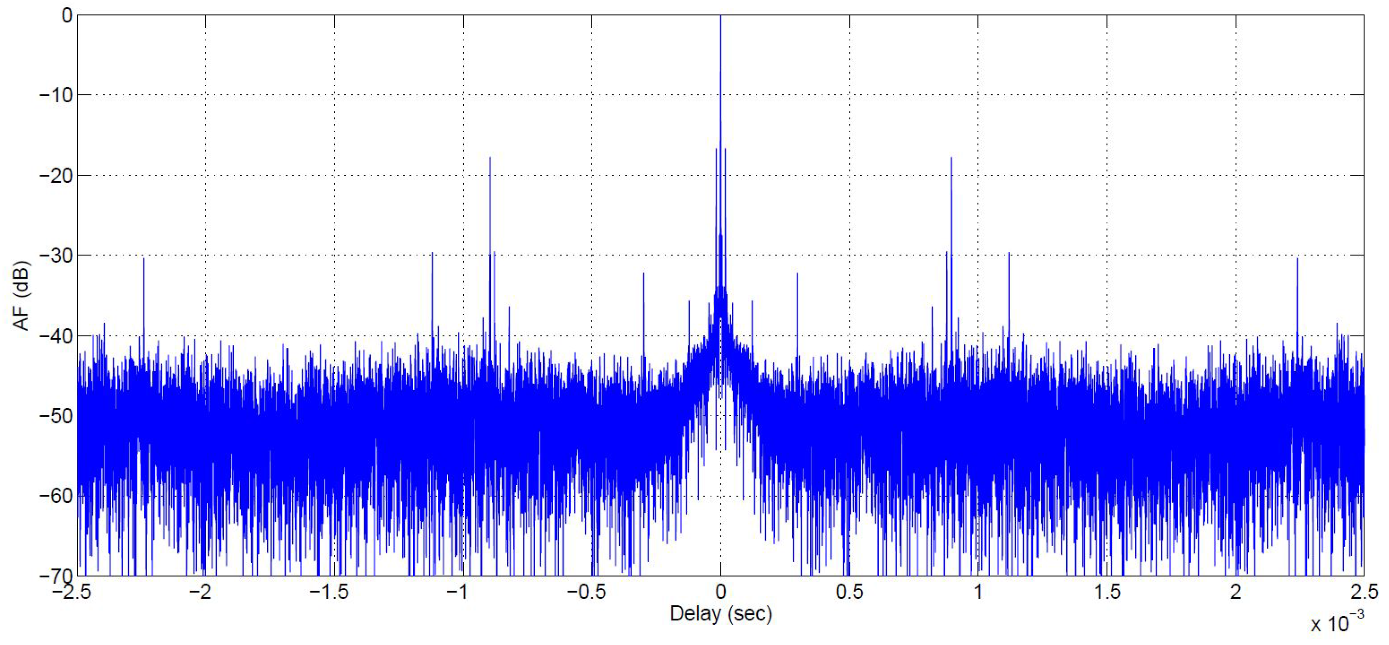
Figure 3.
Zero-Doppler cut of the Ambiguity Function (AF) of a simulated Digital Video Broadcasting-Terrestrial (DVB-T) signal.
Figure 3.
Zero-Doppler cut of the Ambiguity Function (AF) of a simulated Digital Video Broadcasting-Terrestrial (DVB-T) signal.
Figure 4.
Functional block diagram of Improved Detection Techniques for Passive Radars (IDEPAR).
Figure 4.
Functional block diagram of Improved Detection Techniques for Passive Radars (IDEPAR).
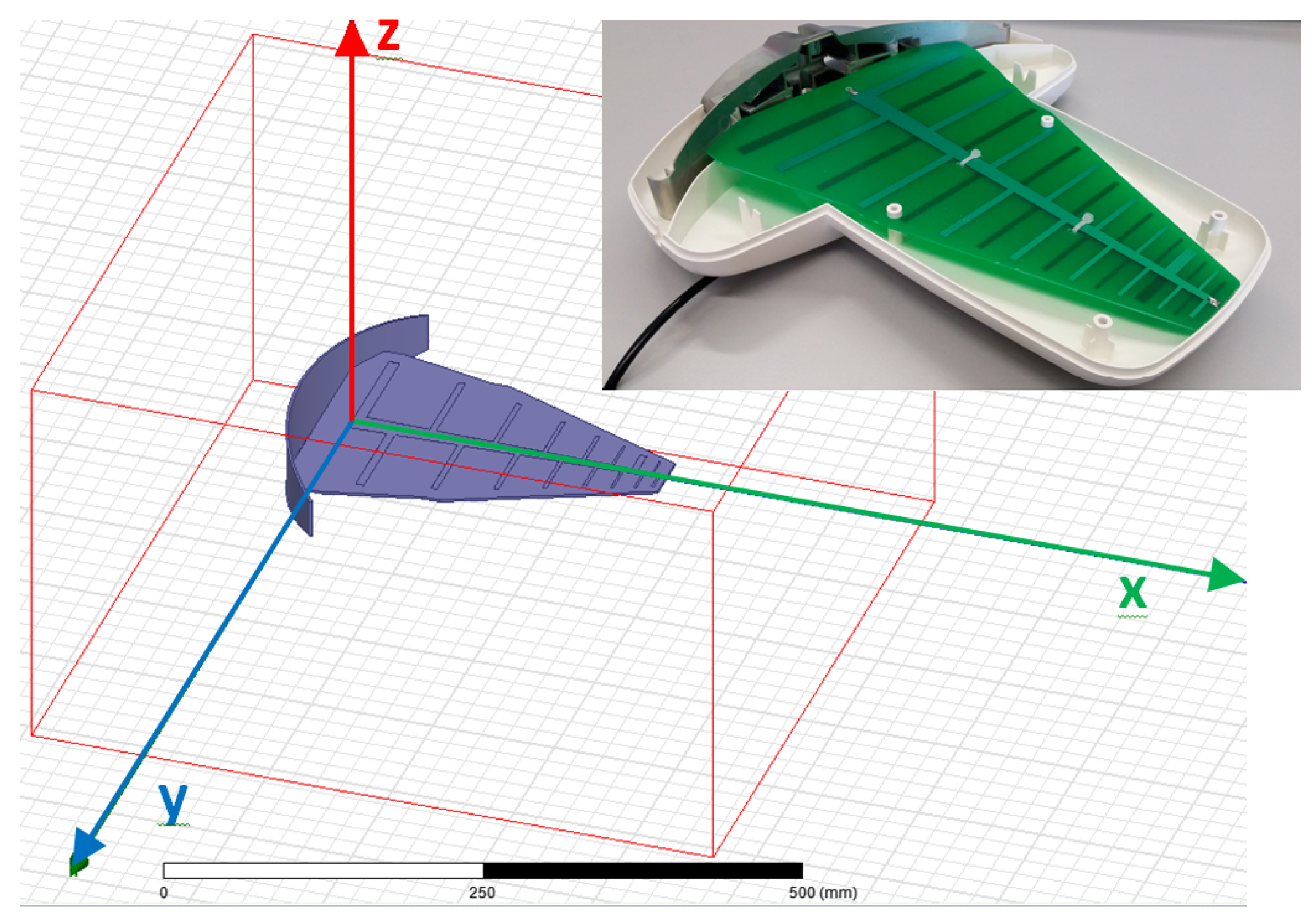
Figure 5.
Televés 4G NOVA antenna.
Figure 5.
Televés 4G NOVA antenna.
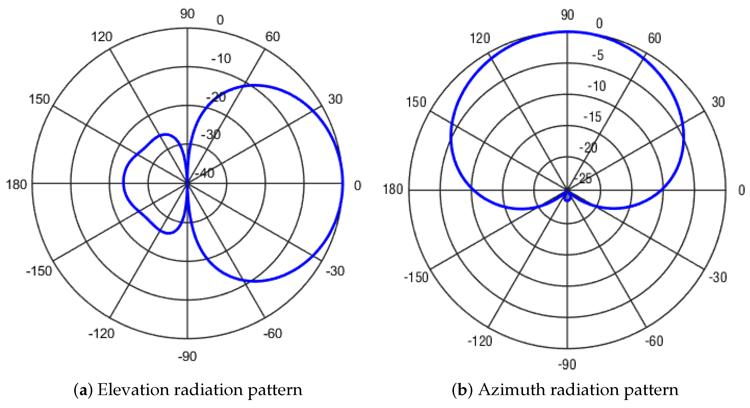
Figure 6.
Televés 4G NOVA antenna radiation pattern generated using ANSYS HFSS.
Figure 6.
Televés 4G NOVA antenna radiation pattern generated using ANSYS HFSS.
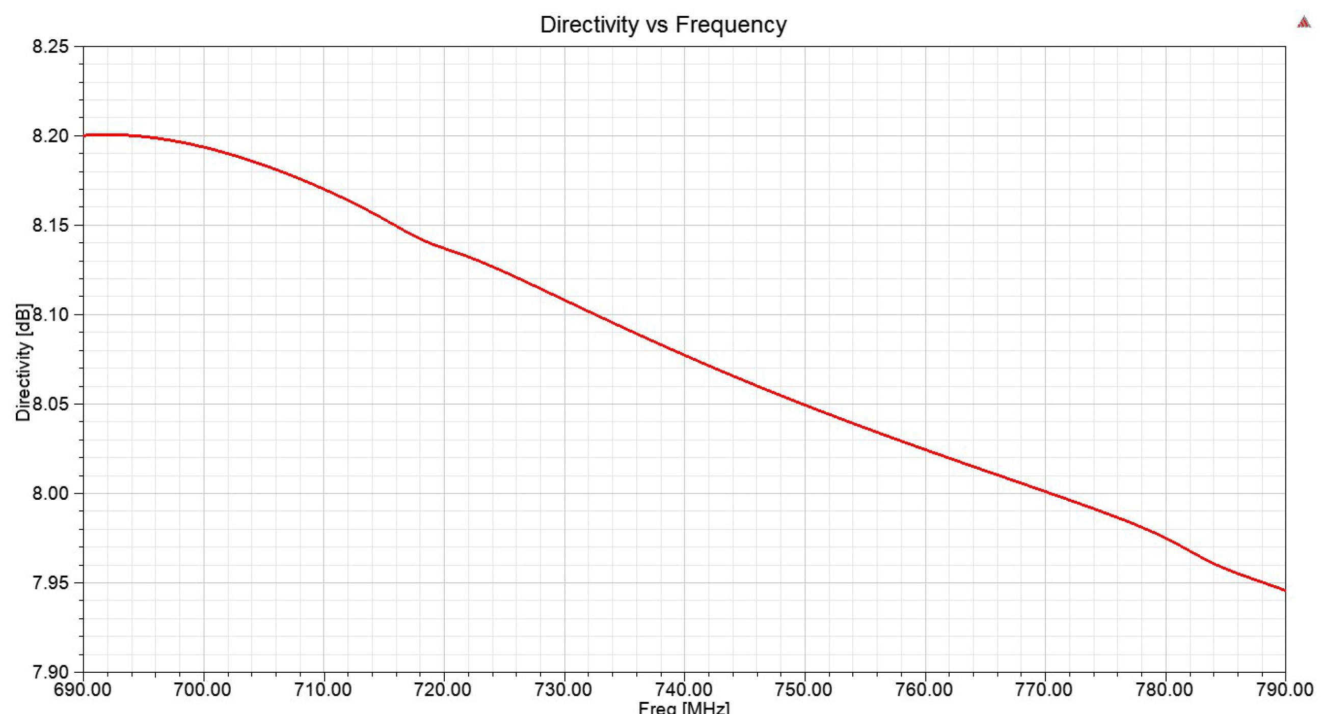
Figure 7.
Gain of the Televés 4G NOVA antenna.
Figure 7.
Gain of the Televés 4G NOVA antenna.
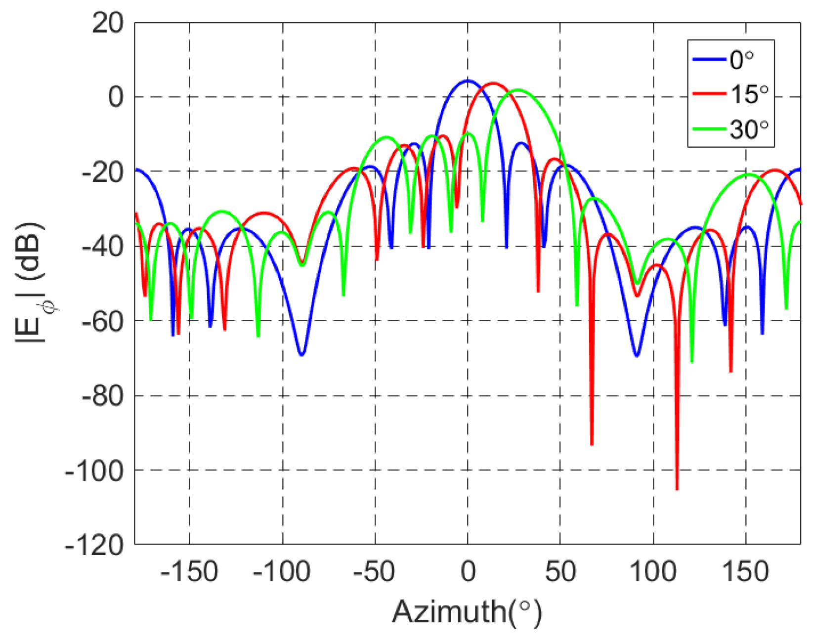
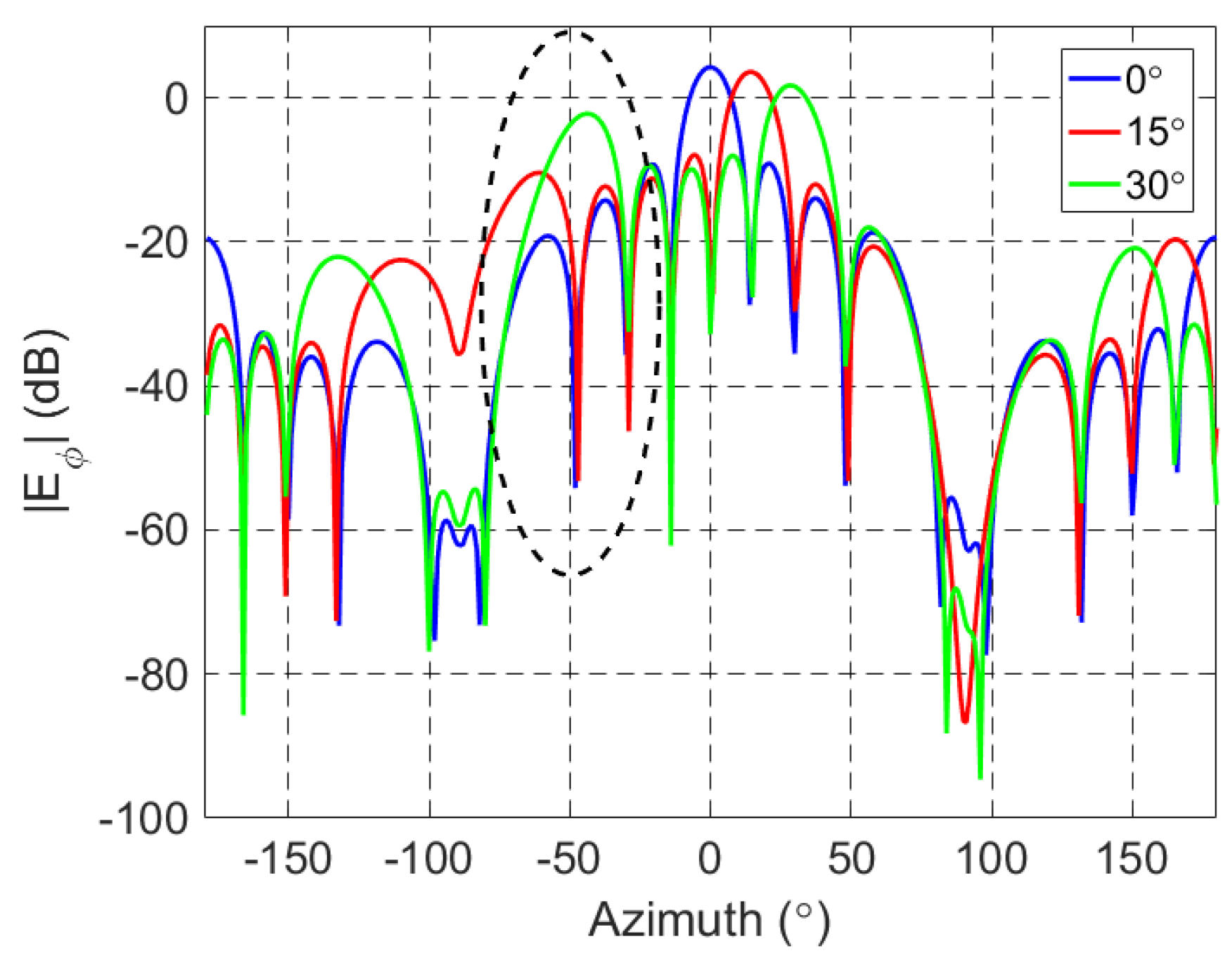
Figure 8.
Azimuth plane radiation pattern of the ULA with five Televes 4G NOVA antennas, for 770 MHz, inter-element spacing equal to 315 mm and three steering directions: (broadside), and . The effect of grating lobes is marked with an ellipse.
Figure 8.
Azimuth plane radiation pattern of the ULA with five Televes 4G NOVA antennas, for 770 MHz, inter-element spacing equal to 315 mm and three steering directions: (broadside), and . The effect of grating lobes is marked with an ellipse.
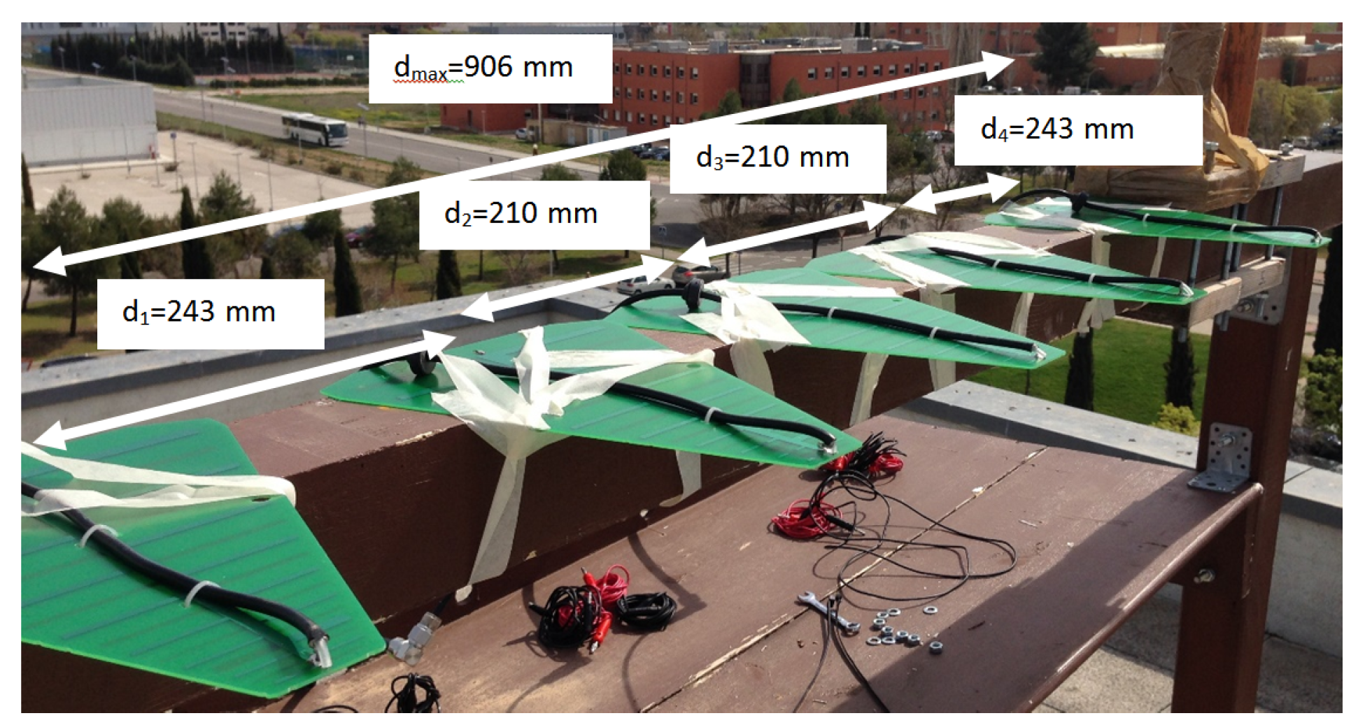
Figure 9.
Designed NULA based on Televés 4G NOVA antennas without the radome detailing the inter-element spacing.
Figure 9.
Designed NULA based on Televés 4G NOVA antennas without the radome detailing the inter-element spacing.
Figure 10.
Azimuth plane radiation pattern of the NULA with five Televes 4G NOVA antennas without the radome or reflector, for 770 MHz, and optimized distances, with three steering directions: (broadside), and .
Figure 10.
Azimuth plane radiation pattern of the NULA with five Televes 4G NOVA antennas without the radome or reflector, for 770 MHz, and optimized distances, with three steering directions: (broadside), and .
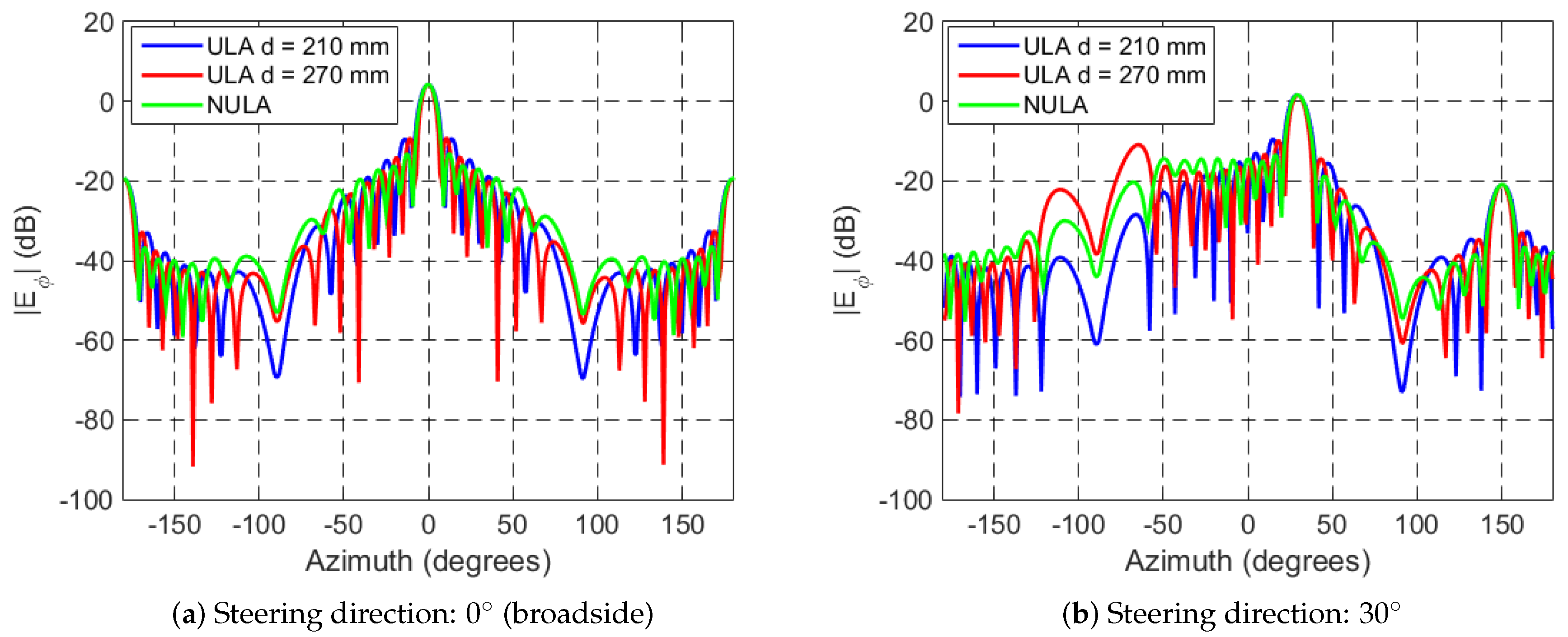
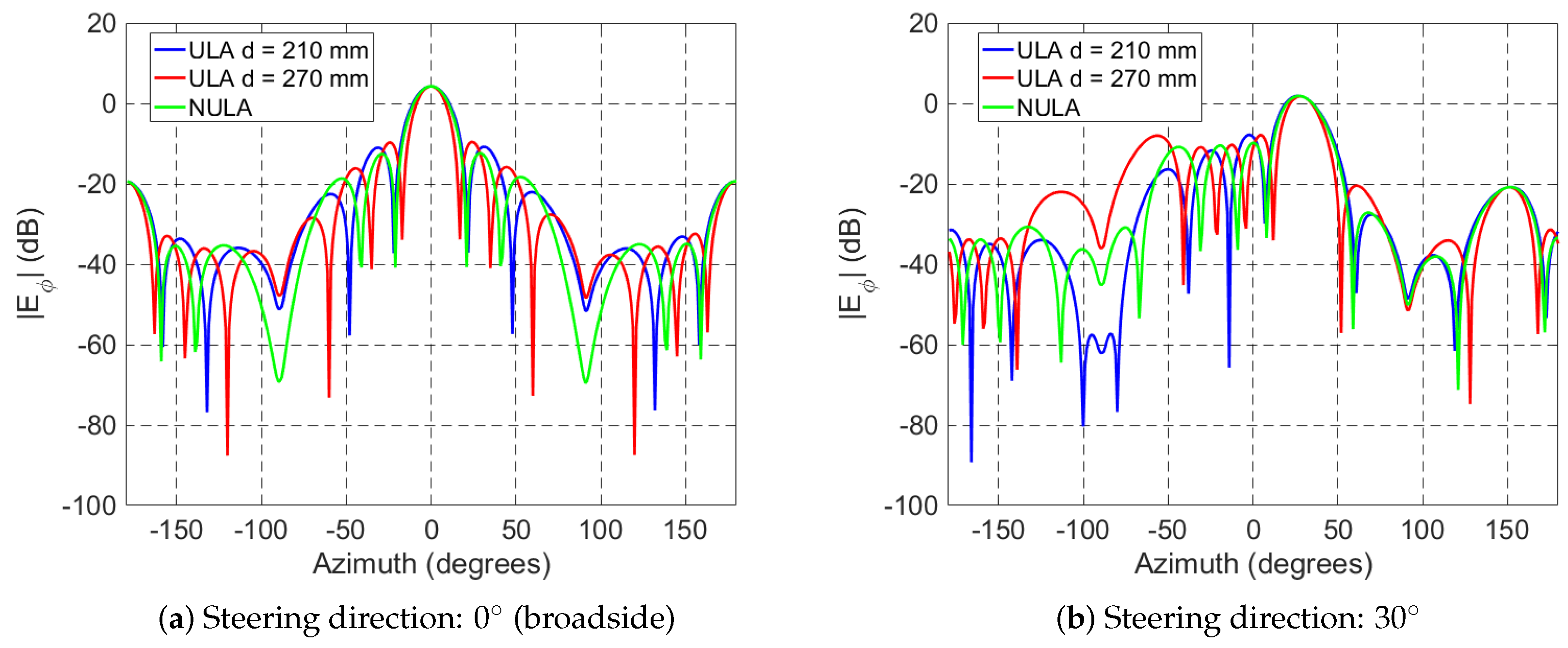
Figure 11.
Azimuth plane radiation patterns of the ULAs (d = 210 mm and 270 mm) and NULA, with five Televes 4G NOVA antennas without the radome or reflector, for 770 MHz.
Figure 11.
Azimuth plane radiation patterns of the ULAs (d = 210 mm and 270 mm) and NULA, with five Televes 4G NOVA antennas without the radome or reflector, for 770 MHz.
Figure 12.
Azimuth plane radiation patterns of the ULAs (d = 210 mm and 270 mm) and NULA, with 11 Televes 4G NOVA antennas without the radome or reflector, for 770 MHz.
Figure 12.
Azimuth plane radiation patterns of the ULAs (d = 210 mm and 270 mm) and NULA, with 11 Televes 4G NOVA antennas without the radome or reflector, for 770 MHz.
Figure 13.
Signals throughout the processing chain previous to the array signal processing stage.
Figure 13.
Signals throughout the processing chain previous to the array signal processing stage.
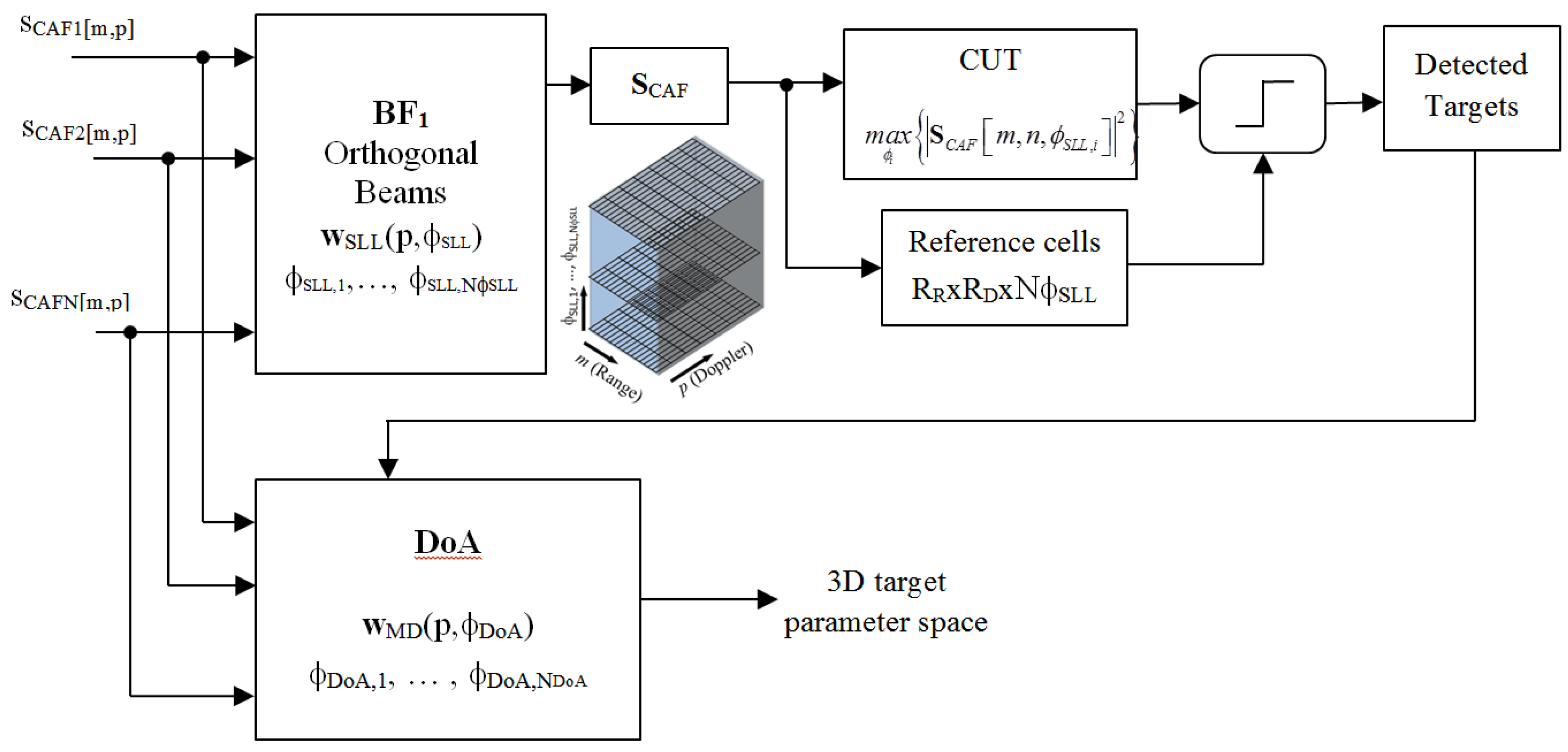
Figure 14.
Two-stage frequency-domain spatial filtering scheme.
Figure 14.
Two-stage frequency-domain spatial filtering scheme.
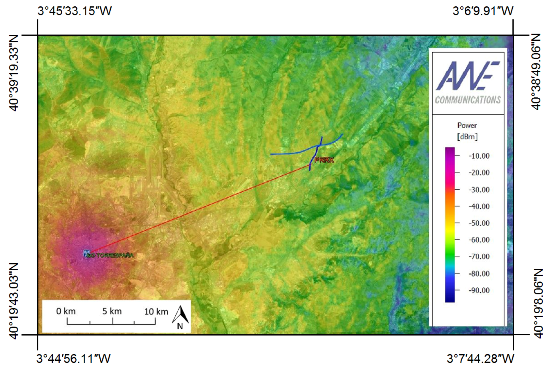
Figure 15.
Received power levels provided by the Torrespaña Illuminator of Opportunity (IoO) in the considered radar scenario.
Figure 15.
Received power levels provided by the Torrespaña Illuminator of Opportunity (IoO) in the considered radar scenario.
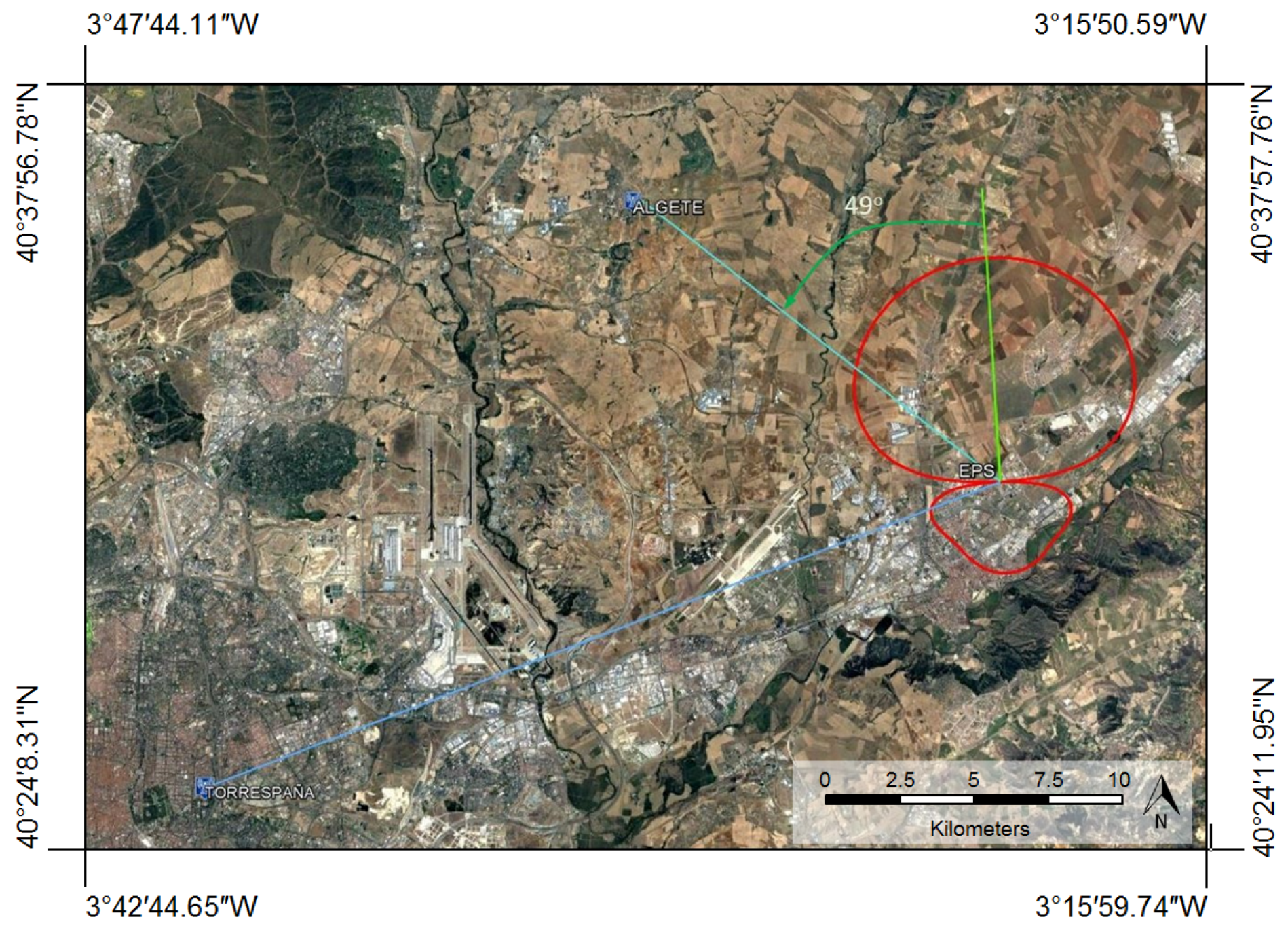
Figure 16.
Radar scenario located at the roof of the Superior Polytechnic School of Alcalá University.
Figure 16.
Radar scenario located at the roof of the Superior Polytechnic School of Alcalá University.
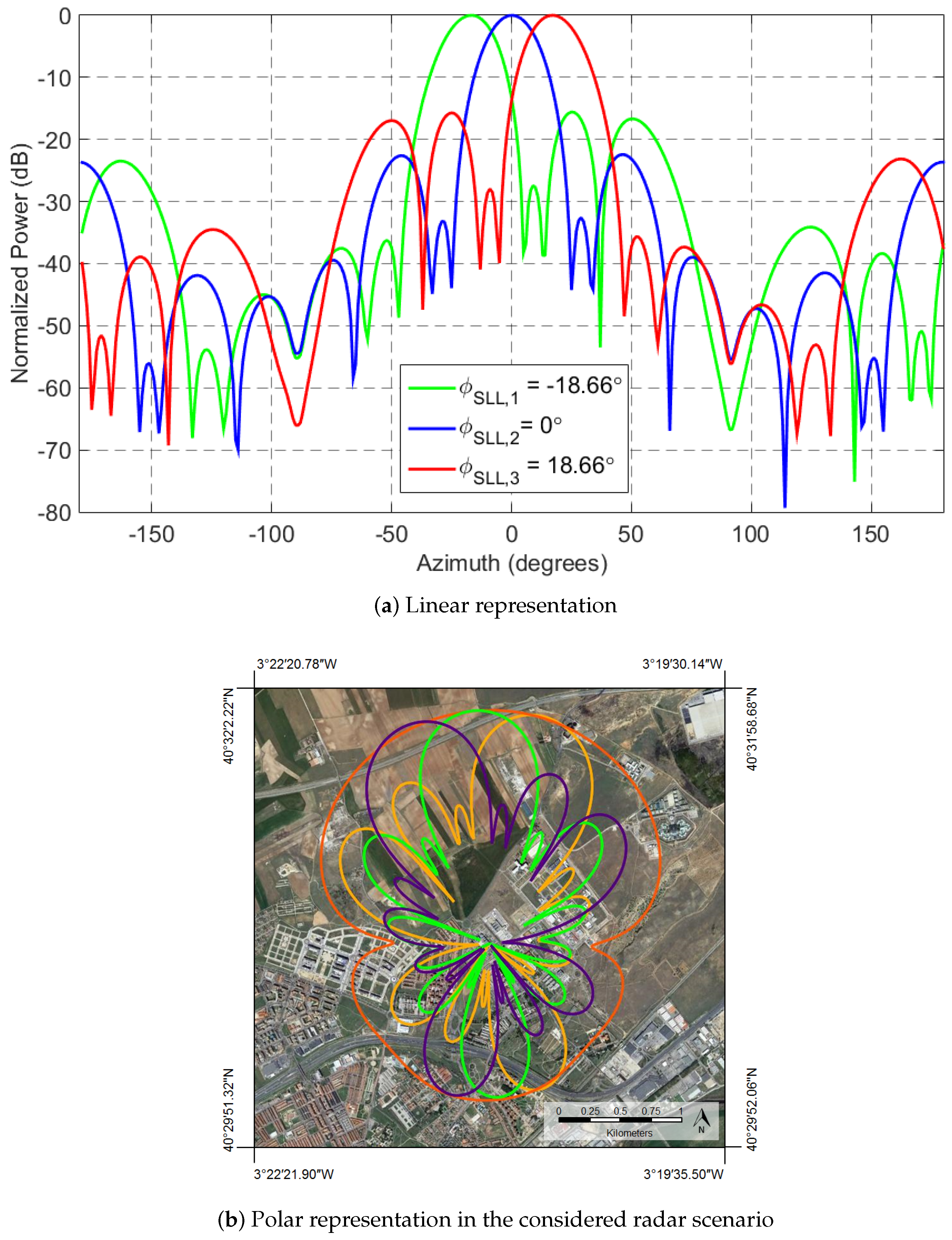
Figure 17.
Azimuth radiation pattern of NULA multiple simultaneous orthogonal beams in the azimuth coverage area φ ∈ [−30°,−30°].
Figure 17.
Azimuth radiation pattern of NULA multiple simultaneous orthogonal beams in the azimuth coverage area φ ∈ [−30°,−30°].
Figure 18.
IDEPAR range coverage in the considered radar scenario. (a) Only one Televés 4G NOVA antenna in the surveillance channel; (b) Televés 4G NOVA antenna array in the surveillance channel.
Figure 18.
IDEPAR range coverage in the considered radar scenario. (a) Only one Televés 4G NOVA antenna in the surveillance channel; (b) Televés 4G NOVA antenna array in the surveillance channel.
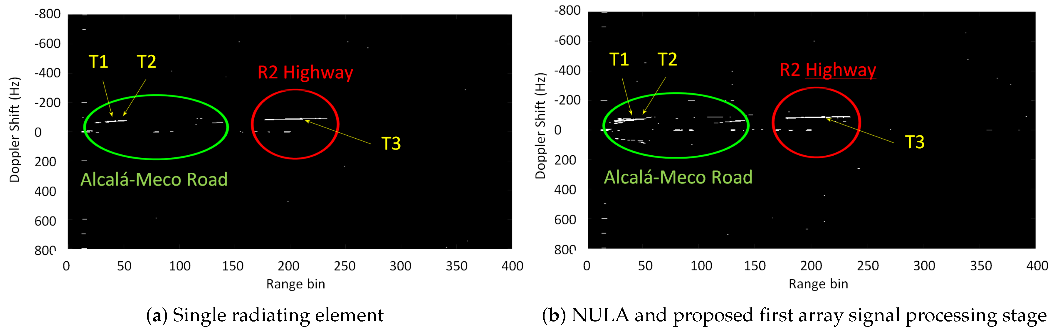
Figure 19.
CFAR detection performance using a single radiating element (a) and the proposed first array signal processing stage applied to the signals acquired by the designed NULA (b).
Figure 19.
CFAR detection performance using a single radiating element (a) and the proposed first array signal processing stage applied to the signals acquired by the designed NULA (b).
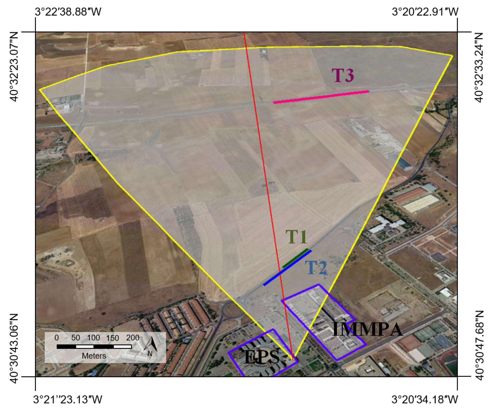
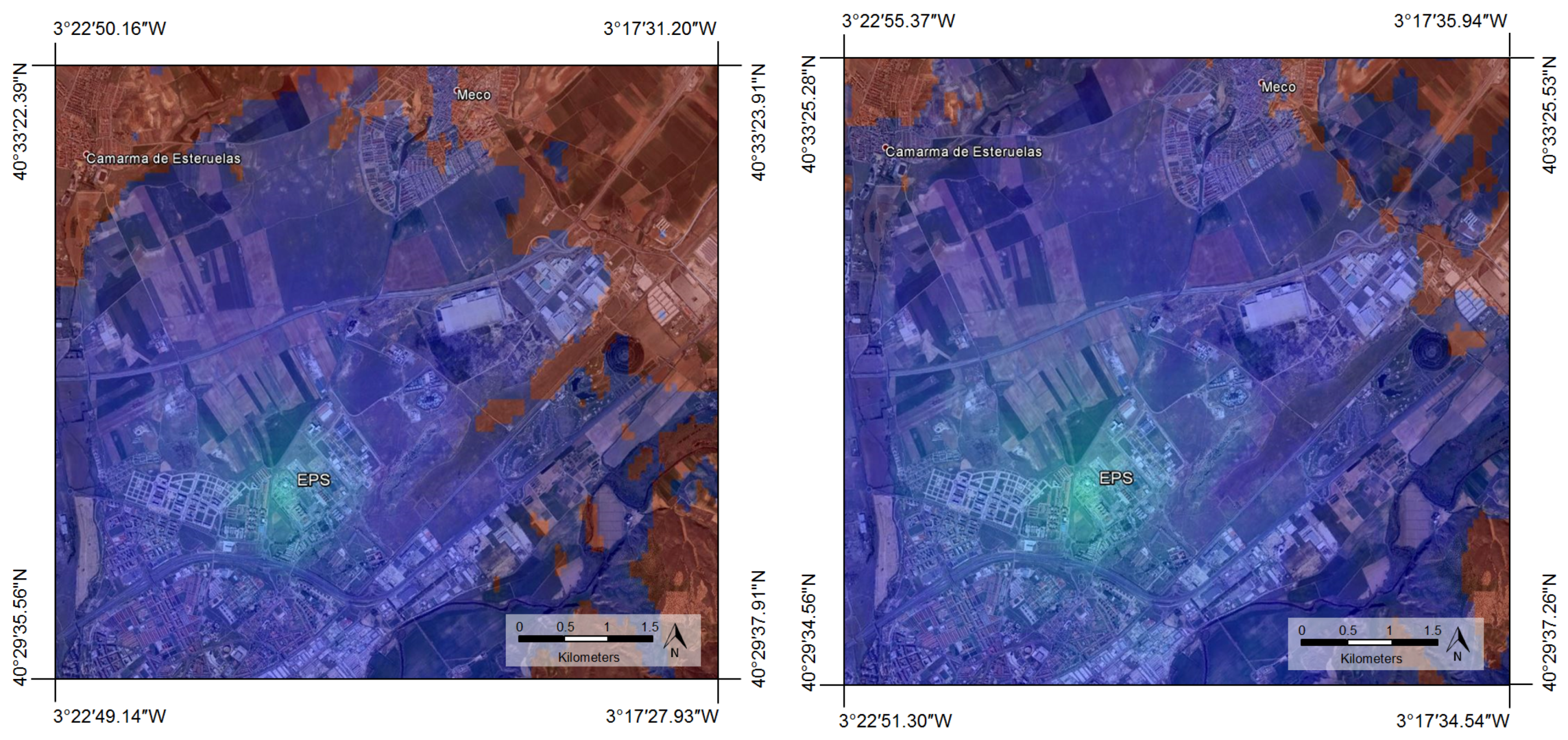
Figure 20.
Targets trajectories in the coverage sector (white). The Polytechnic School of University of Alcalá (EPS, Escuela Politécnica Superior) and a big building made of aluminum (IMMPA, Instituto de Medicina Molecular Príncipe de Asturias) are marked in purple.
Figure 20.
Targets trajectories in the coverage sector (white). The Polytechnic School of University of Alcalá (EPS, Escuela Politécnica Superior) and a big building made of aluminum (IMMPA, Instituto de Medicina Molecular Príncipe de Asturias) are marked in purple.
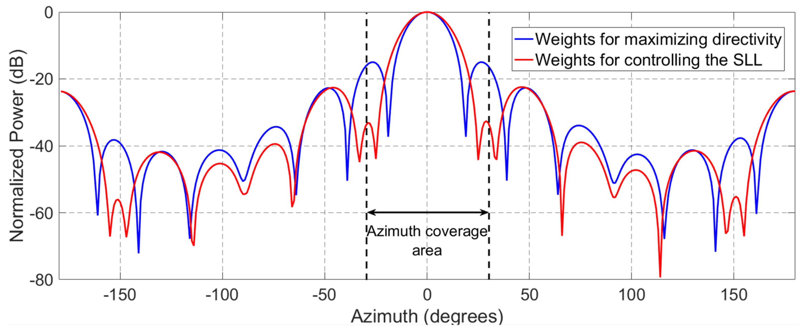
Figure 21.
Comparison of azimuth radiation patterns of NULA with weights calculated for maximizing the directivity (blue) and for guaranteeing dB (red).
Figure 21.
Comparison of azimuth radiation patterns of NULA with weights calculated for maximizing the directivity (blue) and for guaranteeing dB (red).
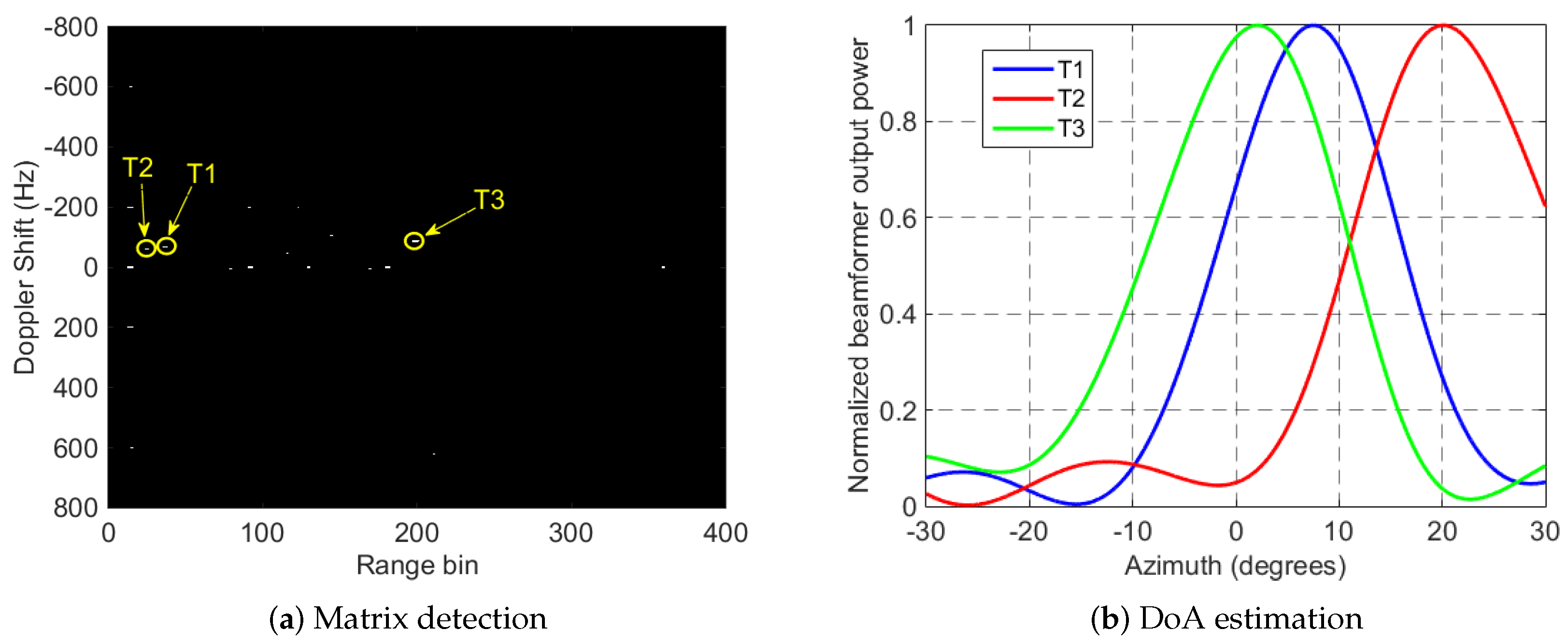
Figure 22.
DoA based on the beamformer output spectrum for detections in the 30th CPI associated with the considered trajectories.
Figure 22.
DoA based on the beamformer output spectrum for detections in the 30th CPI associated with the considered trajectories.
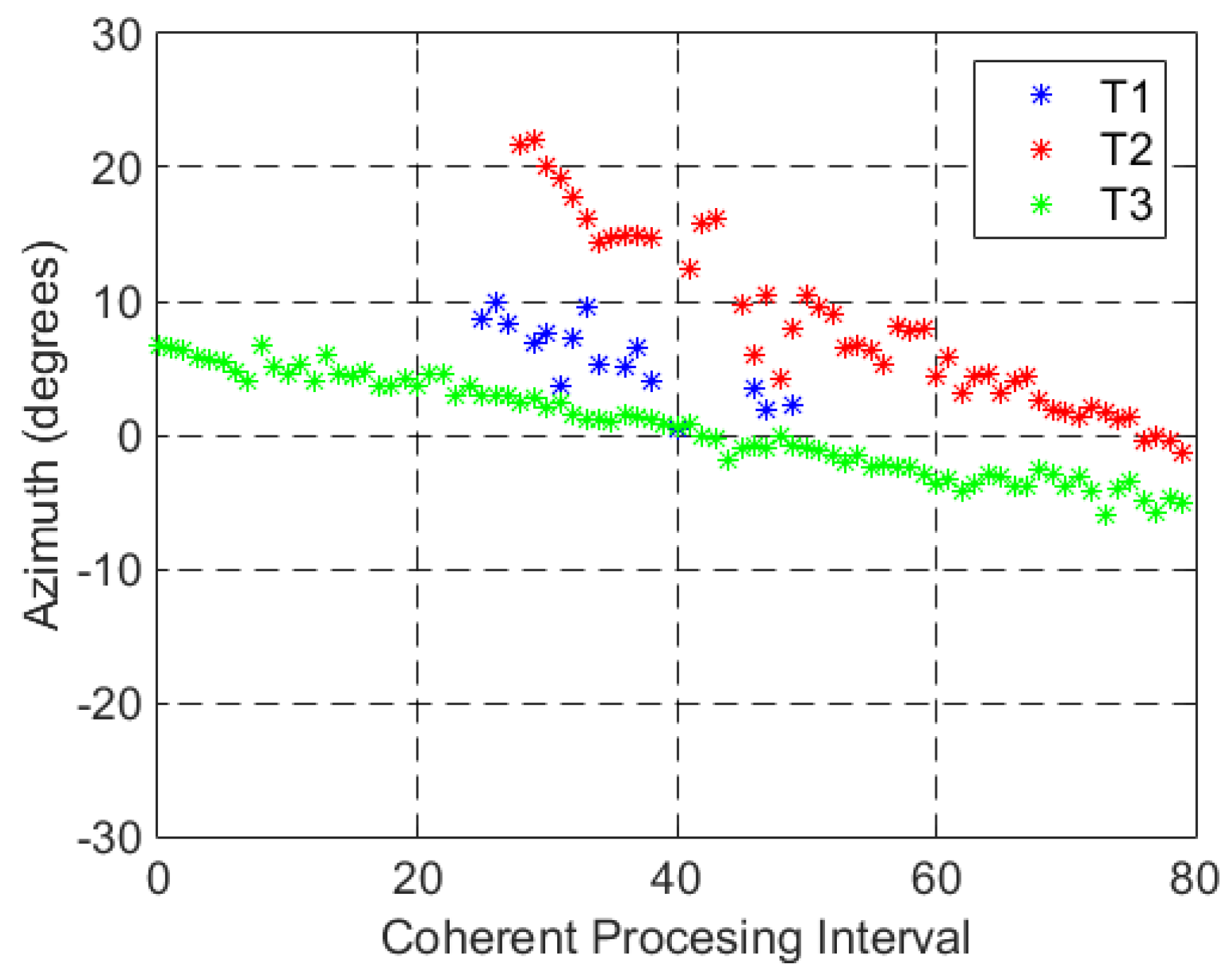
Figure 23.
DoA based on the beamformer output spectrum for targets , and .
Figure 23.
DoA based on the beamformer output spectrum for targets , and .
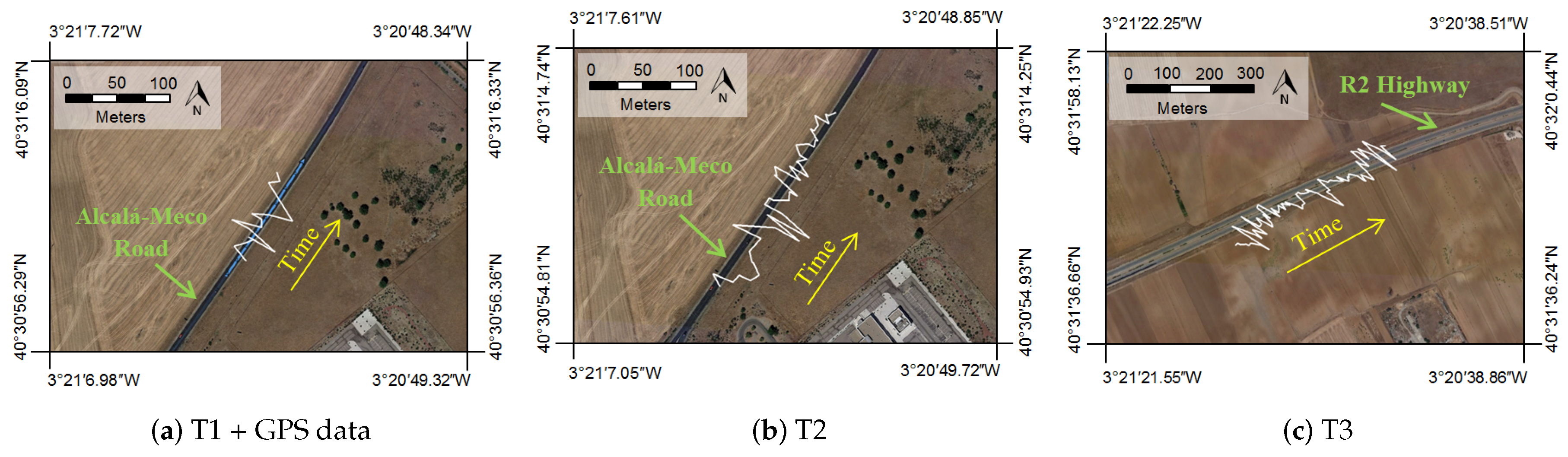
Figure 24.
2D estimated trajectories and GPS data in the radar scenario.
Figure 24.
2D estimated trajectories and GPS data in the radar scenario.
Table 1.
Ambiguity peaks location in the range domain for the 2 k and 8 k modes, due to Guard Interval (GI), Pilot Carriers (PC) and Transport Parameter Signaling (TPS).
Table 1.
Ambiguity peaks location in the range domain for the 2 k and 8 k modes, due to Guard Interval (GI), Pilot Carriers (PC) and Transport Parameter Signaling (TPS).
| Mode | GI Peaks (km) | Scattered PC (km) | Continual PC (km) | TPS (km) |
|---|
| 2 k, | Every | Every & | Every & | |
| 8 k, | Every | Every & | Every & | |
Table 2.
Main characteristics of azimuth plane radiation patterns using conventional weighting of the ULAs with inter-element distances of 210 mm and 270 mm, and a Non-ULA (NULA) with N = 5 elements. The considered steering angles are . SLL, Sidelobe Level; BW, Bandwidth; GLL, Grating Lobe Level.
Table 2.
Main characteristics of azimuth plane radiation patterns using conventional weighting of the ULAs with inter-element distances of 210 mm and 270 mm, and a Non-ULA (NULA) with N = 5 elements. The considered steering angles are . SLL, Sidelobe Level; BW, Bandwidth; GLL, Grating Lobe Level.
| Pointing Angle | Array | BW | SLL (dB) | GLL (dB) | D (dBi) |
|---|
| ULA ( mm) | | 9.43 | x | 12.73 |
| ULA ( mm) | | 9.5 | 9.16 | 13.21 |
| No ULA | | 12.01 | 12.18 | 12.90 |
| ULA ( mm) | | 12.12 | x | 12.86 |
| ULA ( mm) | | 11.57 | x | 13.78 |
| No ULA | | 13.94 | x | 13.13 |
| ULA ( mm) | | 15.06 | x | 12.93 |
| ULA ( mm) | | 13.84 | x | 13.87 |
| No ULA | | 16.62 | x | 13.20 |
| ULA ( mm) | | 12.29 | x | 12.88 |
| ULA ( mm) | | 11.7 | x | 13.80 |
| No ULA | | 14.09 | x | 13.15 |
| ULA ( mm) | | 9.68 | x | 12.72 |
| ULA ( mm) | | 9.64 | 9.75 | 13.21 |
| No ULA | | 11.66 | 12.67 | 12.90 |
Table 3.
Main characteristics of azimuth plane radiation patterns using conventional weighting of the ULAs with inter-element distances of 210 mm and 270 mm and an NULA with N = 11 elements. The considered steering angles are .
Table 3.
Main characteristics of azimuth plane radiation patterns using conventional weighting of the ULAs with inter-element distances of 210 mm and 270 mm and an NULA with N = 11 elements. The considered steering angles are .
| Pointing Angle | Array | BW | SLL (dB) | GLL (dB) | D (dBi) |
|---|
| ULA ( mm) | | 10.98 | x | 15.93 |
| ULA ( mm) | | 11.25 | 11.68 | 16.60 |
| No ULA | | 15.06 | x | 16.14 |
| ULA ( mm) | | 12.25 | x | 16.07 |
| ULA ( mm) | | 12.32 | x | 17.09 |
| No ULA | | 16.25 | x | 16.50 |
| ULA ( mm) | | 13.62 | x | 16.15 |
| ULA ( mm) | | 13.41 | x | 17.18 |
| No ULA | | 17.44 | x | 16.61 |
| ULA ( mm) | | 12.33 | x | 16.09 |
| ULA ( mm) | | 12.38 | x | 17.11 |
| No ULA | | 16.32 | x | 16.52 |
| ULA ( mm) | | 11.09 | x | 15.92 |
| ULA ( mm) | | 11.35 | 12.52 | 16.58 |
| No ULA | | 15.16 | x | 16.13 |
Table 4.
Main characteristics of the azimuth plane radiation patterns generated with maximum directivity weighting vectors of the ULAs with inter-element spacings of 210 mm and 270 mm and the NULA designed in
Section 3.2, for
N = 5 commercial antennas. The considered steering angles are
.
Table 4.
Main characteristics of the azimuth plane radiation patterns generated with maximum directivity weighting vectors of the ULAs with inter-element spacings of 210 mm and 270 mm and the NULA designed in
Section 3.2, for
N = 5 commercial antennas. The considered steering angles are
.
| Pointing Angle | Array | BW | SLL (dB) | GLL (dB) | D (dBi) |
|---|
| ULA ( mm) | | 9.62 | x | 12.73 |
| ULA ( mm) | | 8.53 | 10.6 | 13.21 |
| NULA | | 9.72 | x | 13.36 |
| ULA ( mm) | | 11.95 | x | 12.86 |
| ULA ( mm) | | 11.23 | x | 13.78 |
| NULA | | 11.76 | x | 13.59 |
| ULA ( mm) | | 15.11 | x | 12.93 |
| ULA ( mm) | | 15.36 | x | 13.87 |
| NULA | | 14.73 | x | 13.71 |
| ULA ( mm) | | 12.12 | x | 12.88 |
| ULA ( mm) | | 11.37 | x | 13.80 |
| NULA | | 11.92 | x | 13.61 |
| ULA ( mm) | | 9.81 | x | 12.72 |
| ULA ( mm) | | 8.68 | 11.24 | 13.21 |
| NULA | | 9.71 | x | 13.36 |
Table 5.
Main characteristics of the azimuth plane radiation patterns generated with the maximum directivity weighting vector of the ULAs with inter-element spacings of 210 mm and 270 mm and the NULA designed in
Section 3.2, for
N = 11 commercial antennas. The considered steering angles are
.
Table 5.
Main characteristics of the azimuth plane radiation patterns generated with the maximum directivity weighting vector of the ULAs with inter-element spacings of 210 mm and 270 mm and the NULA designed in
Section 3.2, for
N = 11 commercial antennas. The considered steering angles are
.
| Pointing Angle | Array | BW | SLL (dB) | GLL (dB) | D (dBi) |
|---|
| ULA ( mm) | | 10.98 | x | 15.93 |
| ULA ( mm) | | 9.69 | 12.26 | 16.60 |
| NULA | | 14.34 | x | 16.06 |
| ULA ( mm) | | 12.25 | x | 16.07 |
| ULA ( mm) | | 12.23 | x | 17.09 |
| NULA | | 13.22 | x | 16.48 |
| ULA ( mm) | | 13.62 | x | 16.15 |
| ULA ( mm) | | 13.39 | x | 17.18 |
| NULA | | 14.68 | x | 16.63 |
| ULA ( mm) | | 12.33 | x | 16.09 |
| ULA ( mm) | | 12.29 | x | 17.11 |
| NULA | | 13.30 | x | 16.5 |
| ULA ( mm) | | 11.09 | x | 15.92 |
| ULA ( mm) | | 9.78 | 13.10 | 16.58 |
| NULA | | 14.44 | x | 16.05 |
Table 6.
Main characteristics of the azimuth plane radiation patterns generated with the SLL control weighting vector of the ULAs with inter-element spacings of 210 mm and 270 mm and the NULA designed in
Section 3.2, for
N = 5 commercial antennas. The considered steering angles are
.
Table 6.
Main characteristics of the azimuth plane radiation patterns generated with the SLL control weighting vector of the ULAs with inter-element spacings of 210 mm and 270 mm and the NULA designed in
Section 3.2, for
N = 5 commercial antennas. The considered steering angles are
.
| Pointing Angle | Array | BW | SLL (dB) | GLL (dB) | D (dBi) |
|---|
| ULA ( mm) | | 15.42 | x | 12.61 |
| ULA ( mm) | | 15.37 | 14.29 | 13.10 |
| NULA | | 15.39 | x | 12.87 |
| ULA ( mm) | | 18.18 | x | 12.58 |
| ULA ( mm) | | 17.49 | x | 13.56 |
| NULA | | 17.9 | x | 12.97 |
| ULA ( mm) | | 21.41 | x | 12.60 |
| ULA ( mm) | | 19.95 | x | 13.60 |
| NULA | | 20.69 | x | 13.03 |
| ULA ( mm) | | 18.36 | x | 12.61 |
| ULA ( mm) | | 17.63 | x | 13.58 |
| NULA | | 18.06 | x | 13 |
| ULA ( mm) | | 15.61 | x | 12.62 |
| ULA ( mm) | | 15.23 | 13.98 | 13.09 |
| NULA | | 15.57 | x | 12.87 |
Table 7.
Main characteristics of the azimuth plane radiation patterns generated with the SLL control weighting vector of the ULAs with inter-element spacings of 210 mm and 270 mm and the NULA designed in
Section 3.2, for
N = 11 commercial antennas. The considered steering angles are
.
Table 7.
Main characteristics of the azimuth plane radiation patterns generated with the SLL control weighting vector of the ULAs with inter-element spacings of 210 mm and 270 mm and the NULA designed in
Section 3.2, for
N = 11 commercial antennas. The considered steering angles are
.
| Pointing Angle | Array | BW | SLL (dB) | GLL (dB) | D (dBi) |
|---|
| ULA ( mm) | | 19.48 | x | 15.49 |
| ULA ( mm) | | 19.72 | 11.24 | 16.23 |
| NULA | | 19.52 | x | 15.66 |
| ULA ( mm) | | 21.03 | x | 15.51 |
| ULA ( mm) | | 20.92 | x | 16.58 |
| NULA | | 23.52 | x | 15.76 |
| ULA ( mm) | | 22.61 | x | 15.57 |
| ULA ( mm) | | 22.21 | x | 16.64 |
| NULA | | 29.08 | x | 15.82 |
| ULA ( mm) | | 21.12 | x | 15.53 |
| ULA ( mm) | | 20.99 | x | 16.60 |
| NULA | | 23.22 | x | 15.78 |
| ULA ( mm) | | 19.61 | x | 15.49 |
| ULA ( mm) | | 19.82 | 12.01 | 16.21 |
| NULA | | 19.65 | x | 15.65 |
Table 8.
IoO and IDEPAR receiver emplacement coordinates.
Table 8.
IoO and IDEPAR receiver emplacement coordinates.
| | Latitude | Longitude | Altitude |
|---|
| Torrespaña transmitter | N | W | 658 m |
| IDEPAR receiver | N | W | 628 m |
Table 9.
Representative average values of the estimated BRCS of the car model selected for the study. BRCS, Bistatic Radar Cross-Section.
Table 9.
Representative average values of the estimated BRCS of the car model selected for the study. BRCS, Bistatic Radar Cross-Section.
| Bistatic Angle | | | | |
|---|
| BRCS | dBsm | dBsm | dBsm | dBsm |
Table 10.
Detection performances evaluated for the controlled car.
Table 10.
Detection performances evaluated for the controlled car.
| | | |
|---|
| Single radiating element | | |
| NULA () | | |
| NULA () | | |
Table 11.
Number of detections with respect to the number of Coherent Processing Intervals (CPIs) associated with the considered trajectories.
Table 11.
Number of detections with respect to the number of Coherent Processing Intervals (CPIs) associated with the considered trajectories.
| | T1 | T2 | T3 |
|---|
| Single radiating element | | | |
| NULA () | | | |
| NULA () | | | |
Table 12.
Signal-to-Interference Ratios (SIR) study for the selected targets.
Table 12.
Signal-to-Interference Ratios (SIR) study for the selected targets.
| | T1 | T2 | T3 |
|---|
| Single radiating element | dB | dB | dB |
| NULA () | dB | dB | dB |
| NULA () | dB | dB | dB |


