
Reconstructing Satellite-Based Monthly Precipitation over Northeast China Using Machine Learning Algorithms


1
Guangzhou Institute of Geography, Guangzhou 510070, China
2
Key Laboratory of Guangdong for Utilization of Remote Sensing and Geographical Information System, Guangzhou 510070, China
3
Guangdong Open Laboratory of Geospatial Information Technology and Application, Guangzhou 510070, China
4
College of Environment and Planning, Henan University, Kaifeng 475004, China
5
State Key Laboratory of Resources and Environmental Information System, Institute of Geographic Sciences and Natural Resources Research, Chinese Academy of Sciences, Beijing 100101, China
*
Author to whom correspondence should be addressed.
Remote Sens. 2017, 9(8), 781; https://doi.org/10.3390/rs9080781
Submission received: 31 May 2017
/
Revised: 12 July 2017
/
Accepted: 26 July 2017
/
Published: 30 July 2017
(This article belongs to the Special Issue Remote Sensing Precipitation Measurement, Validation, and Applications)
Abstract
:Attaining accurate precipitation data is critical to understanding land surface processes and global climate change. The development of satellite sensors and remote sensing technology has resulted in multi-source precipitation datasets that provide reliable estimates of precipitation over un-gauged areas. However, gaps exist over high latitude areas due to the limited spatial extent of several satellite-based precipitation products. In this study, we propose an approach for the reconstruction of the Tropical Rainfall Measuring Mission (TRMM) 3B43 monthly precipitation data over Northeast China based on the interaction between precipitation and surface environment. Two machine learning algorithms, support vector machine (SVM) and random forests (RF), are implemented to detect possible relationships between precipitation and normalized difference vegetation index (NDVI), land surface temperature (LST), and digital elevation model (DEM). The relationships between precipitation and geographical location variations based on longitude and latitude are also considered in the reconstruction model. The reconstruction of monthly precipitation in the study area is conducted in two spatial resolutions (25 km and 1 km). The validation is performed using in-situ observations from eight meteorological stations within the study area. The results show that the RF algorithm is robust and not sensitive to the choice of parameters, while the training accuracy of the SVM algorithm has relatively large fluctuations depending on the parameter settings and month. The precipitation data reconstructed with RF show strong correlation with in situ observations at each station and are more accurate than that obtained using the SVM algorithm. In general, the accuracy of the estimated precipitation at 1 km resolution is slightly lower than that of data at 25 km resolution. The estimation errors are positively related to the average precipitation.
1. Introduction
Precipitation is a significant factor affecting surface drought and wetness conditions, ecosystem health, and regional environment change [1,2]. Precipitation data are the basic observation items of meteorological stations. For a long time, meteorological ground observation stations have mainly been used to observe precipitation. Today, with the improvements in observation technology, ground precipitation stations are automated and fundamental for the precipitation observation system [3,4]. However, the observation site can only reflect the precipitation information of limited discrete points. The individual site can only represent the precipitation within a certain radius around the location, especially in complex terrains, which is influenced by local environmental factors. Acquiring precipitation observations over mountainous and underdeveloped regions is therefore still difficult due to the sparse rain gauge network.
The development of satellite technologies revolutionized the observations and acquisition of precipitation information, and enriched the data sources for precipitation observations [5,6,7,8,9,10,11,12,13,14]. Remote sensing has been the main tool for the estimation of precipitation, and several satellite-based precipitation datasets have been developed [15], such as the Global Precipitation Climatology Project (GPCP) [12], Global Satellite Mapping of Precipitation Project (GSMaP) [16], Climate Prediction Center (CPC) Morphing method (CMORPH) [17], Meteosat Visible and Infrared Imager (MVIRI) [18], and the Tropical Rainfall Measuring Mission (TRMM) [19,20]. Among those remote sensing precipitation datasets, the TRMM satellite (equipped with the first active microwave sensor dedicated to detect precipitation) and the TRMM precipitation datasets have provided reliable data on water cycles for ecological models and environmental and climate change studies [21].
However, acquiring precipitation datasets over regions without satellite coverage is still challenging. For example, the spatial coverage of existing global satellite-based TRMM precipitation datasets is 50° S to 50° N. The question therefore arises whether the application of the satellite precipitation datasets may be limited by its spatial extents in global climate modeling. Hydrologic modeling applications might also be restricted over high-latitude areas, especially in areas with sparse in situ networks for precipitation measurements. There are various methods, including multiple linear regression, machine learning, time series analysis, and interpolation techniques that have been used to fill gaps in climatic variables, such as streamflow, total water storage changes, air temperature, and soil moisture [22,23,24]. However, they have not been widely used for the reconstruction of satellite-based precipitation. Due to the temporal and spatial complexity of precipitation itself and the complex relationship with other influencing factors, simple fitting algorithms or image restoration methods based on an image itself are difficult to use and the resulting products are unreliable. Therefore, auxiliary information might be introduced into the reconstruction process.
Selecting appropriate land surface characteristics that are strongly related to precipitation is the primary issue. Those datasets must be easily accessible and widely covered. Previous studies acknowledged the response of vegetation to precipitation [25,26,27,28]; vegetation can also influence the development of moist convection both locally and on scales of ten to thousands of kilometers [2,29]. Multiple studies reported the co-variability between surface temperature and precipitation [30,31]. When the ground is wet, more energy likely contributes to evaporation. If the ground is wet due to rainfall, the associated clouds block the sun, reducing the energy and temperature. Furthermore, high rates of evaporation could occur directly from bare soil after periods of rain, further suppressing the sensible heat and surface temperature [32,33]. Therefore, remote sensing vegetation indices (e.g., the Normalized Difference Vegetation Index, NDVI) and land surface temperature (LST) are often used to monitor dry and wet surface state [25,27,28,34,35]. Moreover, the topography could also have great impact on the regional atmospheric circulation and spatial pattern of precipitation [36,37]. In theory, an increase in the elevation could increase the relative humidity of air masses by expanding and cooling arising air masses, resulting in precipitation [38]. Globally covered NDVI, LST, and digital elevation model (DEM) products with fine spatial resolution provide reliable remote sensing data. These data products are all released online and are easily accessible.
The purpose of this study is to develop an approach for the estimation of precipitation over regions that are not covered by satellite-based precipitation datasets. Based on the relationship between precipitation and NDVI, LST and DEM, we constructed estimation models using machine learning algorithms, and conducted a case study over regions in Northeast China that are uncovered by TRMM 3B43 precipitation data.
2. Study Area and Data Resources
2.1. Study Area
China is located in the eastern part of Asia at the western Pacific coast, between 20°13′ N and 53°34′ N, 73° E and 135°05′ E, covering a total area of 9.6 million km2. China’s climate is mainly dominated by dry seasons and wet monsoons [39,40], which lead to pronounced precipitation and temperature differences between winter and summer [41]. The study area, with a total area of 175,546 km2, is located in the northern part of Northeast China (Figure 1). The region is in the high latitudes and belongs to the cold temperate zone. Precipitation data from eight meteorological ground stations in the study area are used for validation (Figure 1b). Based on in situ observations, the average annual precipitation in the study area is 448.5 mm. The wettest month is July (monthly average precipitation is 123.7 mm), while the driest month is February (monthly average precipitation is 4.2 mm).
2.2. Data Resources
The remote sensing precipitation data were obtained from the Tropical Rainfall Measuring Mission (TRMM), which is a research satellite launched in 1997 for monitoring precipitation over the tropical and sub-tropical regions [19]. The original spatial resolution of precipitation data obtained from TRMM is 0.25° × 0.25°, and the spatial coverage of products is 50° N–50° S. The datasets used in this study are monthly precipitation data from the version 7 of TRMM 3B43 product (TRMM 3B43 V7) of 2003, 2006 and 2009 (http://pmm.nasa.gov/TRMM/trmm-instruments). The original data were projected to the Albers Conical Equal Area projection and the spatial resolution of the data was resampled to 25-km.
The monthly NDVI and land surface temperature (LST) datasets were obtained from Moderate Resolution Imaging Spectroradiometer (MODIS) products that acquired with Terra (https://lpdaac.usgs.gov/). These products with original sinusoidal projection were re-projected to the Albers Conical Equal Area projection. The spatial resolution of the data was maintained at 1 km.
The DEM data were obtained from the NASA Shuttle Radar Topographic Mission (SRTM) (http://srtm.csi.cgiar.org/) [42]. DEM data with 30 and 90m spatial resolutions are available. The data with 90 m spatial resolution were downloaded considering the spatial scales of this study. Then the data were re-sampled to 1 km using an average algorithm by averaging the values of all pixels within each 1 km pixel.
3. Methods
3.1. Precipitation Reconstruction Algorithm
The basic idea of the reconstruction method in this study is to build estimation models using samples extracted from available TRMM 3B43 pixels; the models are established based on the relationship between precipitation and land surface characteristics. In this study, we considered NDVI, daytime LST (LSTday), nighttime LST (LSTnight), day-night LST difference (LSTDN), and DEM as land surface characteristics. The land surface characteristics datasets over the study area were then used as input for the established model to estimate the precipitation over the un-covered region. This method is based on the assumption that the machine learning algorithm can simulate the relationship between precipitation and land surface characteristics with high accuracy. This simulation model can be used to estimate the precipitation over regions that were uncovered by the precipitation datasets.
Relationships between precipitation and the surface conditions may vary widely from one environment to another and from one region to another. Therefore, to establish a robust reconstructing model, sufficient training datasets were required to guarantee that there are enough training samples. Meanwhile, concerning the spatial heterogeneity of precipitation, we included geo-locations (latitude and longitude) as independent variables. In this study, we used the TRMM data covering the China land area as input dependent variable samples, and land surface temperature, NDVI, DEM, and geo-locations (latitude and longitude) were input as independent variables. The process of the approach can be described as follows:
- (1)
- In regions covered with snow, water bodies, and desert, the NDVI values are usually constant under 0.0. To eliminate the influence of snow and water bodies, the threshold NDVI < 0.0 was used to distinguish and remove snow, and water body pixels from original monthly NDVI images.
- (2)
- The LSTDN was calculated by subtracting LSTnight from LSTday; NDVI1km, DEM1km, LSTday-1km, LSTnight-1km, LSTDN-1km were resampled to 25 km resolution using an average method. The geographical coordinates of the center of each 25 × 25 km grid were extracted.
- (3)
- The relationship between the resampled independent variables and TRMM 3B43 V7 precipitation data were established using machine learning algorithms. In this study, we tested two machine learning algorithms for simulating the monthly precipitation, support vector machine (SVM) and random forests (RF).
- (4)
- The reconstruction of monthly precipitation in the study area was conducted on two scales. First, the resampled independent variables (NDVI, DEM, LSTday, LSTnight and LSTDN ) with 25 km spatial resolution were input into the established model. Reconstructed results of 25 km resolution were achieved. Second, the 1 km spatial resolution precipitation can be simulated by applying the established model to the variables with original 1 km spatial resolution.
3.2. Support Vector Machine (SVM)
The SVM is an outstanding machine learning algorithm for classification and regression problems, and has been successfully applied in different fields such as soil moisture estimation [43], impervious surface estimation [44] and biophysical parameter estimation from remote sensing data [45]. The original SVM algorithm was invented by Vladimir Vapnik and his co-workers in the early 1990s for classification problems, and then was extended to the case of regression [46,47]. The basic idea of the SVM algorithm is derived from optimization theory that uses a hyper-plane to classify the input variables into an m-dimensional feature space with maximal margin. The maximal margin is derived by solving the constrained dual problem:
where are independent variables, is dependent variables, C is the capacity parameter cost, and i = 1, …., L is the sample size and the approximating function is given by
where and are Lagrange multipliers, and b is the “bias” term; and is the kernel function that measures non-linear dependence between the two input variables x, and xi. The xi’s are “support vectors”, and N (usually ) is the number of selected data points or support vectors corresponding to values of the independent variable that are at least away from actual observations. The training pattern in the dual formulation can be used to estimate the dot product of two vectors of any dimensions and is regarded as the advantage of the dual formulation. This advantage in SVM is used to deal with non-linear function approximations.
Selecting a suitable kernel function and kernel parameter are important steps involved in SVM modeling. In this study, we selected the Radial Basis Function (RBF) as the kernel. The RBF kernel function is given by
where is specified by keyword gamma, must be greater than 0.
Thus, when training an SVM with the RBF kernel, two parameters must be considered: C and gamma. The parameter C, common to all SVM kernels, trades off misclassification of training examples against simplicity of the decision surface. A low C makes the decision surface smooth, while a high C aims at classifying all training examples correctly. The gamma defines how much influence a single training example has. The larger gamma is, the closer other examples must be to be affected. Interested readers are referred to Kalra and Ahmad [48] for the illustration of the working mechanism and an example of the SVM technique.
3.3. Random Forests (RF)
Random Forests (RF) as an non-parameter and ensemble learning algorithm for regression and classification had been increasingly applied and was reported to yield high accuracy and be robust to outliers [49]. The RF, which was proposed by Breiman [50], is a combination of tree predictors such that each tree depends on the values of a randomly chosen subset of input variables vectors sampled independently and with the same distribution for all trees in the forests [50]. The tree predictor is based on the classification and regression trees (CART) algorithm [51]. The basic idea of CART is to construct a tree-like graph or model of decisions and their possible consequences. It generates relative homogeneous subgroups by recursively partitioning the training dataset to the maximum variance between groups of independent and dependent variables. In each of the terminal nodes of the tree, a simple and accurate model is built to explain the relationship of independent and dependent variables. The RF regression algorithm process can be briefly described as follows:
- (1)
- The ntree (number of trees) samples sets are randomly drawn from the original training sample set with replacement. Each sample set is a bootstrap sample, and the elements that are not included in the bootstrap are termed “out-of-bag data” (OOB) for that bootstrap sample.
- (2)
- For each bootstrap sample, an un-pruned regression tree is grown with the modification that a random subset of the variables, from which the best variables are split, is selected at each node.
- (3)
- Predictions for new samples can be made by averaging the predictions from all the individual regression trees:where N is the number of trees, is the prediction from each individual regression tree.
4. Results and Analysis
4.1. Performance of Regression Algortihms
The selected algorithms are openly accessible and easy to use; they are clearly documented elsewhere. Sources of the codes are implemented in scikit-learn, which is a Python package integrating a wide range of state-of-the-art machine learning algorithms for medium-scale supervised and unsupervised problems [52]. The establishment of the RF and SVM based models largely depends on certain parameterizations, and the choice of optimal parameters is significant. In practice, we conducted experiments to cover a majority range of parameter combinations for each algorithm [50,51,52,53,54,55,56,57] (Table 1). A grid search algorithm was implemented to find the optimal parameters for each algorithm. The grid search exhaustively considers all parameter combinations with a cross-validation scheme. We used a k-fold strategy, which divides all the samples in k groups of samples, called folds, of equal sizes. The prediction function is learned using k-1 folds, and the fold left out is used for test. In this study, we used default k value 3.
The SVM and RF model were trained by using the same datasets with 25 km spatial resolution. All available pixels covering China land area were used as samples, including 14,893 pixels for each month. Figure 2 shows the training accuracy of the two algorithms under different parameter conditions. The accuracy of the SVM algorithm is greatly influenced by the gamma parameter, and the Cost has less effect on the accuracy of the algorithm. When the gamma changes in the range of [2−6, 26], the R2 gradually increases and then decreases, and reaches the maximums when gamma = 24 and gamma = 25. It can be seen that the accuracy of the SVM algorithm with the parameter setting changes shows relatively large fluctuations. This indicates that SVM is sensitive to the choice of parameters. For the RF algorithm, when the number of trees (n_estimators) changes within [20, 200], the average fitting accuracy of the algorithm continues to rise, and gradually stabilize when n_estimators is larger than 100. It can be seen that although the accuracy of RF algorithm fitting increases with the number of trees, the R2 has been at a high level when using the various parameters. The average R2 is greater than 0.99. This indicates that the RF algorithm is not sensitive to the choice of parameters and is robust. Table 2 shows the average R2, mean absolute error (MAE), and the root mean squared error (RMSE) of the two algorithms for each month. It can be seen that the training accuracy of SVM varies in different months, while the R2 of RF for each month are all greater than 0.99 for each month.
4.2. Reconstruction Results
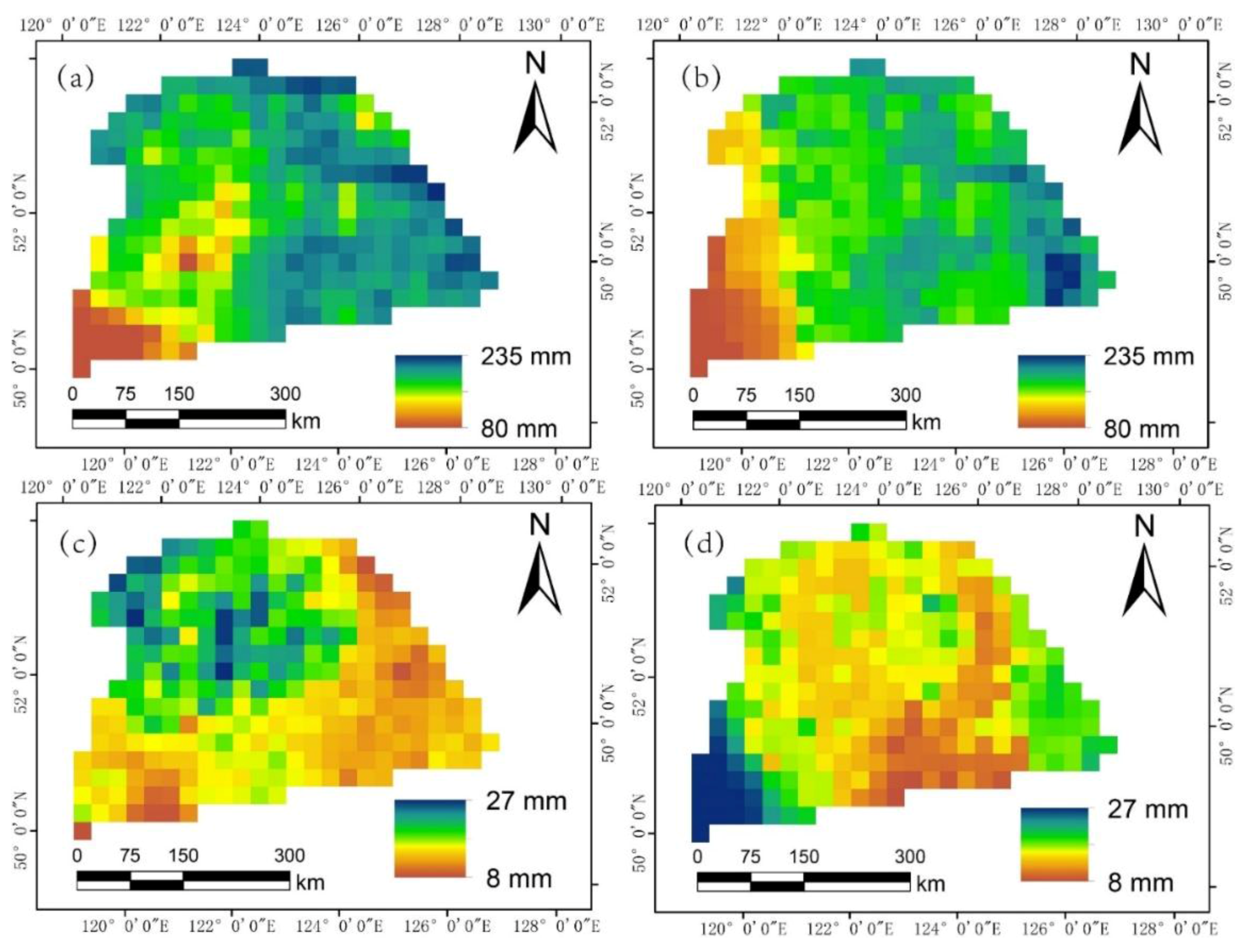
The estimated results at 25 km resolution for June and October of 2009 are presented in Figure 3. The results estimated at 1 km resolution for January, June and October are presented in Figure 4. Based on the visual comparison, the results at 1 km resolution provide more detailed spatial information compared with the results of 25 km resolution. The estimated results of TRMM 3B43 precipitation using SVM and RF show quite different spatial distribution characteristics.
4.3. Validation and Error Analysis
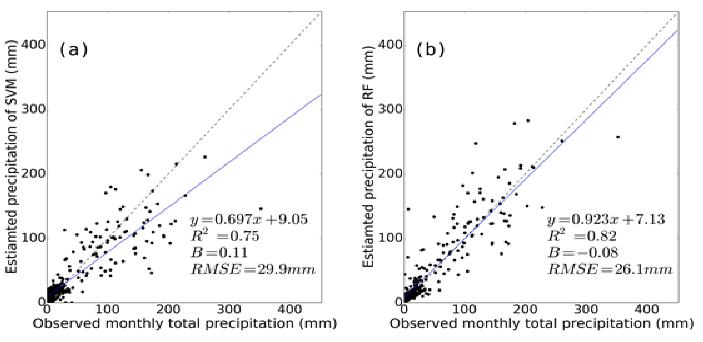
The results with coarse (25 km) and fine (1 km) spatial resolution were validated with observations from eight meteorological stations in the study area. Figure 5 shows the scatter plots of the results with coarse resolution and the observations for each algorithm; Figure 6 presents the scatter plots of the results with fine resolution and the observations for each algorithm.
It can be seen that the results obtained using the RF algorithm at 25 km and 1 km resolution are more accurate than that of the SVM. The estimated precipitation based on RF strongly correlates with the in situ observations; R2 of RF is larger than 0.8. However, the accuracy of the precipitation estimated at 1 km resolution is slightly lower than that at 25 km resolution.
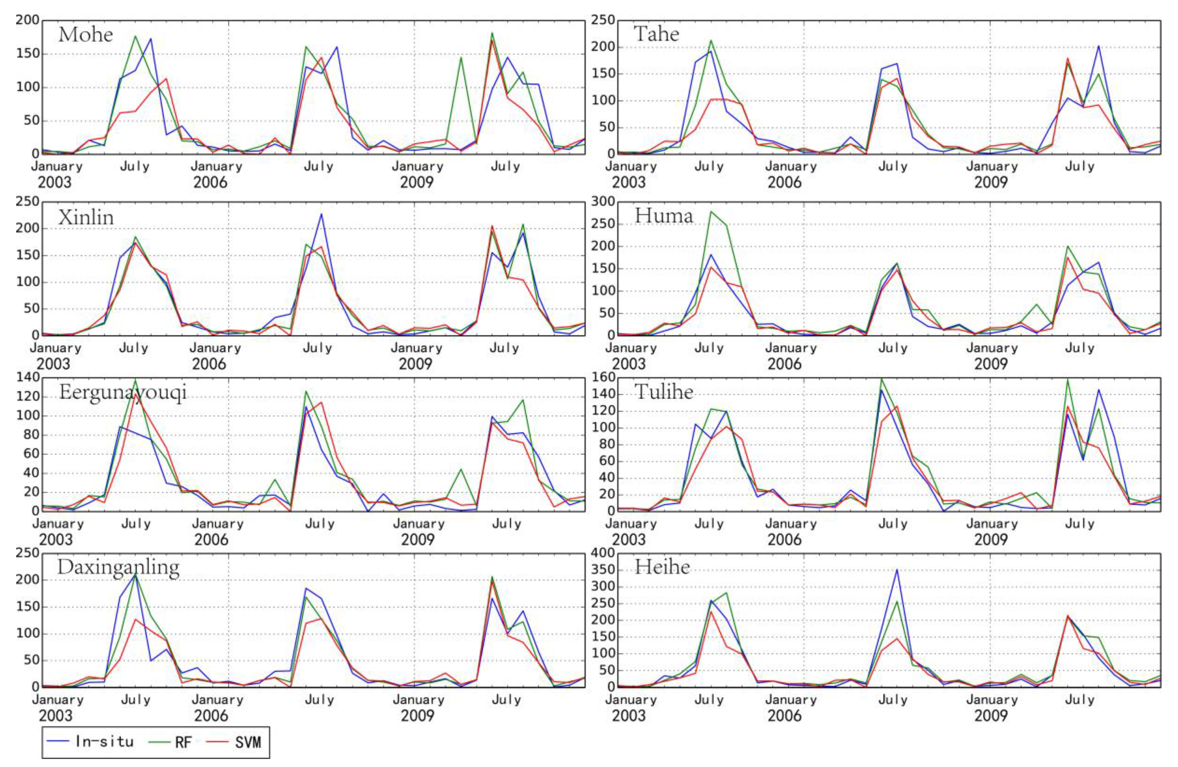
We examined the temporal behavior of the in situ measurements and the precipitation reconstructed at eight stations during the entire period (the results at 1 km spatial resolution are displayed in Figure 7). Except for individual months, the reconstruction results are in good agreement with the site observations. The precipitation estimated at the eight sites accurately reflects annual and inter-annual variations of the precipitation; the results obtained from the RF algorithm are closer to the observations.
Table 3 and Table 4 show the R2, RMSE, and Bias between observations and estimated monthly precipitation of 25 km and 1 km resolution at eight stations, respectively. Accurate precipitation estimates were obtained at each station. According to Table 3, with respect to the results at 25 km resolution, the R2 of the RF algorithm is higher than that of the SVM algorithm at each station, ranging from 0.72 to 0.93. The R2 values of Eergunayouqi, Tulihe, Daxinganling, and Heihe are larger than 0.9. The RMSE of the RF algorithm at each site is lower than that of the SVM algorithm. However, the Bias of the RF algorithm is larger than that of the SVM algorithm at five stations (Mohe, Tahe, Huma, Tulihe, and Daxinganling).
In general, the RF algorithm shows a higher accuracy than the SVM at 1 km resolution for each individual station. However, the SVM performed better than RF at the Huma Station. Except for the Mohe Station, the estimated precipitation is in good agreement with the observations, with R2 higher than 0.8. The best agreement was observed at the Heihe Station (R2 = 0.91), followed by Tulihe (R2 = 0.90). Overall, the RF algorithm tends to underestimate the monthly precipitation, with a negative Bias; the Bias reached −0.24 and −0.18 at the Huma and Eergunanyouqi stations, respectively.
To investigate the relationship between the estimation errors and precipitation observations, we calculated the average MAE of the reconstructed results for each station and the average precipitation observations of the stations (Figure 8). In general, the estimation errors positively correlate with the average precipitation; the MAEs increase with increasing average precipitation. The MAE of the SVM model increases at a rate of 2.6 mm/10 mm (R2 = 0.43); the MAE increase rate of the RF model was 2.2 mm/10 mm (R2 = 0.35). These results indicate that the errors increase as the total monthly precipitation increases and that the rate of increase of RF is lower than that of the SVM.
5. Discussion
5.1. Scale Sensitivity of the Model
In this study, we rebuilt precipitation data for Northeast China. The reconstructing models were established at 25 km resolution. The scale effect is one of the most important issues in remote sensing research. The information and characteristics reflected by different scales might be completely different. The same model might produce completely different results at different spatial scales. Based on Immerzeel et al. (2009) and Jia et al. (2011), models established based on precipitation and NDVI/DEM might have different accuracies at different spatial scales. To explore the scale sensitivity of the reconstruction model, we established models at 25 km, 50 km, 75 km, and 100 km resolution based on the two machine learning algorithms. The simulation abilities of the models were analyzed at different scales.
Figure 9 shows the simulation accuracy (R2 and RMSE) of the two machine learning algorithms based on four different scales. The R2 and RMSE of the different scales are quite similar. This indicates that the machine learning algorithm of the reconstruction model is not affected by scale changes. In addition, the RF-based model has a higher accuracy at each scale and in each month; however, Figure 9d shows that the accuracy of the RF-based model decreases from 25 to 100 km. Therefore, it is reasonable to establish the reconstruction model at the 25 km scale. If the model is established at a larger scale (50 km to 100 km), the original TRMM data need to be scaled up, which will cause the loss of spatial information and introduce uncertainty to the reconstruction model.
5.2. Influence Factors of the Reconstructing Model
The factors influencing the precipitation are complex and diverse. The factors affecting the accuracy of the precipitation reconstruction model also vary, including various environmental factors considered in the reconstruction model and the accuracy of multi-source remote sensing information.
The TRMM precipitation products have been the focus of research and applications due to the high data quality and accuracy. In theory, the accuracy of reconstruction results largely depends on the accuracy of the original satellite precipitation data. Although TRMM 3B43 V7 precipitation products show a high consistency with in situ observations, the accuracy of the TRMM data might vary during different seasons and from one region to another. Multiple studies showed that the satellite precipitation datasets have a limited ability in estimating trace and solid precipitation. Therefore, the accuracy of reconstructed precipitation might be lower during winter.
The response of vegetation to precipitation has been extensively studied. Water is an important factor affecting the growth of vegetation. Therefore, NDVI, as the best indicator of vegetation growth, has been widely used in precipitation monitoring. Figure 10 shows the in situ observed precipitation and NDVI values at eight stations during the entire period. Figure 11 presents the in situ observed precipitation and land surface temperature values at eight stations. According to the figures, there are positive relationships between precipitation and the NDVI and LST variables. Compared with the land surface temperature, the variation curve of NDVI agrees well with the change of precipitation. However, both the LST and NDVI cannot be consistent with changes in precipitation in some individual months. There are limitations by using NDVI and LST as indicator variables. The NDVI and LST cannot objectively reflect the real precipitation change due to human and natural factors. For example, harvesting and irrigating farmland artificially changes the NDVI and surface temperature, and defoliation of vegetation might worsen the relationship between precipitation and NDVI, LST. The NDVI and LST changes caused by human intervention and natural factors are not controlled by precipitation. In addition, NDVI cannot effectively reflect the change of precipitation in sparsely vegetated areas (NDVI is a constant smaller than or close to zero) and lush vegetation areas (NDVI saturation). The NDVI and surface temperature data are transient data, reflecting the transient state of the surface environment; however, the impact of precipitation on the surface environment is continuous. Although those data have been composited by calculating maximum and average values, data gaps and quality issues caused by clouds and atmospheric conditions still exist, which have an impact on the accuracy of reconstruction results.
6. Conclusions
In this study, a reconstruction algorithm is proposed for monthly TRMM 3B43 precipitation based on machine learning algorithms. The reconstruction is performed over Northeast China at two spatial resolutions (25 km and 1 km). The reconstructed precipitation is validated with in situ observations of eight meteorological stations in the study area.
Based on the training results, the RF algorithm produces a higher training accuracy than the SVM. Moreover, the accuracy of the SVM is greatly affected by the selection of parameters and varies in different months. In contrast, the RF produces a consistent and high accuracy. This indicates that the RF algorithm is more robust than the SVM. The validation results show that the reconstructed monthly precipitation based on RF is more accurate than the results obtained from the SVM. The results estimated by RF show high correlations with the in situ observations for each station and the estimated precipitation at eight stations accurately reflects annual and interannual variations. In general, the RF algorithm outperforms the SVM with respect to the reconstruction model.
The relationship between the estimations errors and precipitation observations was analyzed by comparing the average MAE with the average precipitation observations at each station. The results show that there is a positive relationship between the absolute error and average precipitation. The absolute errors increase as the monthly total precipitation increases, while the rate of increase of RF is lower than that of SVM.
The scale effect is important for remote sensing models. We also analyzed the scale sensitivity of the reconstruction model by comparing the accuracy of the models established at different scales (25 km, 50 km, 75 km, and 100 km). The results show that the training accuracies are quite similar at different scales, indicating that the reconstruction model is not affected by scale changes.
Acknowledgments
This work was jointly supported by the National Natural Science Foundation of China (41601175), the Foundation and Advanced Technology Research Plan of Henan Province (152300410067), the University Science and Technology Innovation Team Support Plan of Henan Province (16IRTSTHN012), the key scientific research project of Henan province (16A610001), the Natural Science Foundation of Guangdong Academy of Sciences (QNJJ201601), the Natural Science Foundation of Guangdong Academy of Sciences (QNJJ201601), GDAS' Special Project of Science and Technology Development(2017GDASCX-0801, 2017GDASCX-0804). The authors are indebted to the National Aeronautics and Space Administration for providing the MODIS, TRMM, and DEM data that were used in this study. We also thank the National Data Sharing Infrastructure of Earth System Science for providing the boundary data of China. In addition, we would like to thank the anonymous reviewers for their helpful comments and suggestions in enhancing this manuscript.
Author Contributions
Wenlong Jing drafted the manuscript and was responsible for the research design, experiment, and analysis. Pengyan Zhang reviewed the manuscript and was responsible for the research design and analysis. Hao Jiang and Xiaodan Zhao supported the data preparation and the interpretation of the results. All of the authors contributed to editing and reviewing the manuscript.
Conflicts of Interest
The authors declare no conflict of interest.
References
- Sapiano, M.R.P.; Arkin, P.A. An intercomparison and validation of high-resolution satellite precipitation estimates with 3-hourly gauge data. J. Hydrometeorol. 2009, 10, 149–166. [Google Scholar] [CrossRef]
- Taylor, C.M.; de Jeu, R.A.M.; Guichard, F.; Harris, P.P.; Dorigo, W.A. Afternoon rain more likely over drier soils. Nature 2012, 489, 423–426. [Google Scholar] [CrossRef] [PubMed] [Green Version]
- Schwaller, M.R.; Morris, K.R. A ground validation network for the global precipitation measurement mission. J. Atmos. Ocean. Technol. 2011, 28, 301–319. [Google Scholar] [CrossRef]
- Schneider, U.; Becker, A.; Finger, P.; Meyer-Christoffer, A.; Ziese, M.; Rudolf, B. Gpcc’s new land surface precipitation climatology based on quality-controlled in situ data and its role in quantifying the global water cycle. Theor. Appl. Climatol. 2014, 115, 15–40. [Google Scholar] [CrossRef]
- Munoz, E.A.; Di Paola, F.; Lanfri, M.; Arteaga, F.J. Observing the troposphere through the advanced technology microwave sensor (atms) to retrieve rain rate. IEEE Lat. Am. Trans. 2016, 14, 586–594. [Google Scholar] [CrossRef]
- Sanò, P.; Panegrossi, G.; Casella, D.; Di Paola, F.; Milani, L.; Mugnai, A.; Petracca, M.; Dietrich, S. The passive microwave neural network precipitation retrieval (pnpr) algorithm for amsu/mhs observations: Description and application to european case studies. Atmos. Meas. Tech. 2015, 8, 837–857. [Google Scholar] [CrossRef]
- Munoz, E.A.; Paola, F.D.; Lanfri, M. Advances on rain rate retrieval from satellite platforms using artificial neural networks. IEEE Lat. Am. Trans. 2015, 13, 3179–3186. [Google Scholar] [CrossRef]
- Di Paola, F.; Ricciardelli, E.; Cimini, D.; Romano, F.; Viggiano, M.; Cuomo, V. Analysis of catania flash flood case study by using combined microwave and infrared technique. J. Hydrometeorol. 2014, 15, 1989–1998. [Google Scholar] [CrossRef]
- Cimini, D.; Romano, F.; Ricciardelli, E.; Di Paola, F.; Viggiano, M.; Marzano, F.S.; Colaiuda, V.; Picciotti, E.; Vulpiani, G.; Cuomo, V. Validation of satellite opemw precipitation product with ground-based weather radar and rain gauge networks. Atmos. Meas. Tech. 2013, 6, 3181–3196. [Google Scholar] [CrossRef]
- Di Paola, F.; Casella, D.; Dietrich, S.; Mugnai, A.; Ricciardelli, E.; Romano, F.; Sanò, P. Combined mw-ir precipitation evolving technique (pet) of convective rain fields. Nat. Hazards Earth Syst. Sci. 2012, 12, 3557–3570. [Google Scholar] [CrossRef] [Green Version]
- Casella, D.; Dietrich, S.; Di Paola, F.; Formenton, M.; Mugnai, A.; Porcù, F.; Sanò, P. Pm-gcd—A combined ir–mw satellite technique for frequent retrieval of heavy precipitation. Nat. Hazards Earth Syst. Sci. 2012, 12, 231–240. [Google Scholar] [CrossRef] [Green Version]
- Huffman, G.J.; Adler, R.F.; Arkin, P.; Chang, A.; Ferraro, R.; Gruber, A.; Janowiak, J.; McNab, A.; Rudolf, B.; Schneider, U. The global precipitation climatology project (gpcp) combined precipitation dataset. Bull. Am. Meteorol. Soc. 1997, 78, 5–20. [Google Scholar] [CrossRef]
- Duan, Z.; Bastiaanssen, W.G.M. First results from version 7 trmm 3b43 precipitation product in combination with a new downscaling–calibration procedure. Remote Sens. Environ. 2013, 131, 1–13. [Google Scholar] [CrossRef]
- Huffman, G.J.; Adler, R.F.; Curtis, S.; Bolvin, D.T.; Nelkin, E.J. Global rainfall analyses at monthly and 3-h time scales. In Measuring Precipitation from Space: Eurainsat and the Future; Levizzani, V., Bauer, P., Turk, F.J., Eds.; Springer: Dordrecht, The Netherlands, 2007; pp. 291–305. [Google Scholar]
- Munchak, S.J.; Skofronick-Jackson, G. Evaluation of precipitation detection over various surfaces from passive microwave imagers and sounders. Atmos. Res. 2013, 131, 81–94. [Google Scholar] [CrossRef]
- Kubota, T.; Shige, S.; Hashizume, H.; Aonashi, K.; Takahashi, N.; Seto, S.; Hirose, M.; Takayabu, Y.N.; Ushio, T.; Nakagawa, K.; et al. Global precipitation map using satellite-borne microwave radiometers by the gsmap project: Production and validation. IEEE Trans. Geosci. Remote Sens. 2007, 45, 2259–2275. [Google Scholar] [CrossRef]
- Joyce, R.J.; Janowiak, J.E.; Arkin, P.A.; Xie, P. Cmorph: A method that produces global precipitation estimates from passive microwave and infrared data at high spatial and temporal resolution. J. Hydrometeorol. 2004, 5, 287–296. [Google Scholar] [CrossRef]
- Bennartz, R.; Schroeder, M. Convective activity over africa and the tropical atlantic inferred from 20 years of geostationary meteosat infrared observations. J. Clim. 2012, 25, 156–169. [Google Scholar] [CrossRef]
- Huffman, G.J.; Bolvin, D.T.; Nelkin, E.J.; Wolff, D.B.; Adler, R.F.; Gu, G.; Hong, Y.; Bowman, K.P.; Stocker, E.F. The trmm multisatellite precipitation analysis (tmpa): Quasi-global, multiyear, combined-sensor precipitation estimates at fine scales. J. Hydrometeorol. 2007, 8, 38–55. [Google Scholar] [CrossRef]
- Asadullah, A.; McIntyre, N.; Kigobe, M.A.X. Evaluation of five satellite products for estimation of rainfall over uganda/evaluation de cinq produits satellitaires pour l’estimation des précipitations en ouganda. Hydrol. Sci. J. 2008, 53, 1137–1150. [Google Scholar] [CrossRef]
- Iguchi, T.; Kozu, T.; Meneghini, R.; Awaka, J.; Okamoto, K.I. Rain-profiling algorithm for the trmm precipitation radar. J. Appl. Meteorl. 2000, 39, 2038–2052. [Google Scholar] [CrossRef]
- Cui, Y.; Long, D.; Hong, Y.; Zeng, C.; Zhou, J.; Han, Z.; Liu, R.; Wan, W. Validation and reconstruction of fy-3b/mwri soil moisture using an artificial neural network based on reconstructed modis optical products over the tibetan plateau. J. Hydrol. 2016, 543, 242–254. [Google Scholar] [CrossRef]
- Coulibaly, P.; Evora, N.D. Comparison of neural network methods for infilling missing daily weather records. J. Hydrol. 2007, 341, 27–41. [Google Scholar] [CrossRef]
- Long, D.; Shen, Y.; Sun, A.; Hong, Y.; Longuevergne, L.; Yang, Y.; Li, B.; Chen, L. Drought and flood monitoring for a large karst plateau in southwest china using extended grace data. Remote Sens. Environ. 2014, 155, 145–160. [Google Scholar] [CrossRef]
- Zhang, X.; Friedl, M.A.; Schaaf, C.B.; Strahler, A.H.; Liu, Z. Monitoring the response of vegetation phenology to precipitation in africa by coupling modis and trmm instruments. J. Geophys. Res.: Atmos. 2005, 110. [Google Scholar] [CrossRef]
- Wang, J.; Price, K.P.; Rich, P.M. Spatial patterns of ndvi in response to precipitation and temperature in the central great plains. Int. J. Remote Sens. 2001, 22, 3827–3844. [Google Scholar] [CrossRef]
- Vicente-Serrano, S.M.; Gouveia, C.; Camarero, J.J.; Beguería, S.; Trigo, R.; López-Moreno, J.I.; Azorín-Molina, C.; Pasho, E.; Lorenzo-Lacruz, J.; Revuelto, J.; et al. Response of vegetation to drought time-scales across global land biomes. Proc. Natl. Acad. Sci. USA 2013, 110, 52–57. [Google Scholar] [CrossRef] [PubMed] [Green Version]
- Zhong, L.; Ma, Y.; Salama, M.S.; Su, Z. Assessment of vegetation dynamics and their response to variations in precipitation and temperature in the tibetan plateau. Clim. Chang. 2010, 103, 519–535. [Google Scholar] [CrossRef]
- Spracklen, D.V.; Arnold, S.R.; Taylor, C.M. Observations of increased tropical rainfall preceded by air passage over forests. Nature 2012, 489, 282–285. [Google Scholar] [CrossRef] [PubMed]
- Lemone, M.A.; Grossman, R.L.; Chen, F.; Ikeda, K.; Yates, D. Choosing the averaging interval for comparison of observed and modeled fluxes along aircraft transects over a heterogeneous surface. J. Hydrometeorol. 2003, 4, 179–195. [Google Scholar] [CrossRef]
- Trenberth, K.E.; Shea, D.J. Relationships between precipitation and surface temperature. Geophys. Res. Lett. 2005, 32. [Google Scholar] [CrossRef]
- De Kauwe, M.G.; Taylor, C.M.; Harris, P.P.; Weedon, G.P.; Ellis, R.J. Quantifying land surface temperature variability for two sahelian mesoscale regions during the wet season. J. Hydrometeorol. 2013, 14, 1605–1619. [Google Scholar] [CrossRef]
- Wallace, J.S.; Holwill, C.J. Soil evaporation from tiger-bush in south-west niger. J. Hydrol. 1997, 188–189, 426–442. [Google Scholar] [CrossRef]
- Kogan, F.N. Application of vegetation index and brightness temperature for drought detection. Adv. Space Res. 1995, 15, 91–100. [Google Scholar] [CrossRef]
- Liu, W.T.; Kogan, F.N. Monitoring regional drought using the vegetation condition index. Int. J. Remote Sens. 1996, 17, 2761–2782. [Google Scholar] [CrossRef]
- Guan, H.; Wilson, J.L.; Xie, H. A cluster-optimizing regression-based approach for precipitation spatial downscaling in mountainous terrain. J. Hydrol. 2009, 375, 578–588. [Google Scholar] [CrossRef]
- Yin, Z.-Y.; Zhang, X.; Liu, X.; Colella, M.; Chen, X. An assessment of the biases of satellite rainfall estimates over the tibetan plateau and correction methods based on topographic analysis. J. Hydrometeorol. 2008, 9, 301–326. [Google Scholar] [CrossRef]
- Sokol, Z.; Bližňák, V. Areal distribution and precipitation–altitude relationship of heavy short-term precipitation in the czech republic in the warm part of the year. Atmos. Res. 2009, 94, 652–662. [Google Scholar] [CrossRef]
- Xu, X.; Lu, C.; Shi, X.; Ding, Y. Large-scale topography of china: A factor for the seasonal progression of the meiyu rainband? J. Geophys. Res. 2010, 115. [Google Scholar] [CrossRef]
- Yang, F.; Lau, K.M. Trend and variability of china precipitation in spring and summer: Linkage to sea-surface temperatures. Int. J. Climatol. 2004, 24, 1625–1644. [Google Scholar] [CrossRef]
- Zhai, P.; Zhang, X.; Wan, H.; Pan, X. Trends in total precipitation and frequency of daily precipitation extremes over china. J. Clim. 2005, 18, 1096–1108. [Google Scholar] [CrossRef]
- Jarvis, A.; Reuter, H.I.; Nelson, A.; Guevara, E. Hole-Filled Srtm for the Globe Version 4. Available online: cgiar-csi srtm 90m database (accessed on 31 January 2016).
- Ahmad, S.; Kalra, A.; Stephen, H. Estimating soil moisture using remote sensing data: A machine learning approach. Adv. Water Resour. 2010, 33, 69–80. [Google Scholar] [CrossRef]
- Weng, Q. Remote sensing of impervious surfaces in the urban areas: Requirements, methods, and trends. Remote Sens. Environ. 2012, 117, 34–49. [Google Scholar] [CrossRef]
- Mountrakis, G.; Im, J.; Ogole, C. Support vector machines in remote sensing: A review. ISPRS J. Photogramm. Remote Sens. 2011, 66, 247–259. [Google Scholar] [CrossRef]
- Vapnik, V. The Nature of Statistical Learning Theory; Springer: New York, NY, USA, 1995. [Google Scholar]
- Vapnik, V. Statistical Learning Theory; Wiley: New York, NY, USA, 1998. [Google Scholar]
- Kalra, A.; Ahmad, S. Using Oceanic-Atmospheric Oscillations for Long Lead Time Streamflow Forecasting; American Geophysical Union: Washington, DC, USA, 2009; pp. 450–455. [Google Scholar]
- Gislason, P.O.; Benediktsson, J.A.; Sveinsson, J.R. Random forests for land cover classification. Pattern Recognit. Lett. 2006, 27, 294–300. [Google Scholar] [CrossRef]
- Breiman, L. Random forests. Mach. Learn. 2001, 45, 5–32. [Google Scholar] [CrossRef]
- Breiman, L.; Friedman, J.H.; Olshen, R.A.; Stone, C.J. Classification and Regression Trees; Chapman and Hall/CRC: Boca Raton, FL, USA, 1984. [Google Scholar]
- Pedregosa, F.; Varoquaux, G.; Gramfort, A.; Michel, V.; Thirion, B.; Grisel, O.; Blondel, M.; Prettenhofer, P.; Weiss, R.; Dubourg, V.; et al. Scikit-learn: Machine learning in python. J. Mach. Learn. Res. 2011, 12, 2825–2830. [Google Scholar]
- Li, C.; Wang, J.; Wang, L.; Hu, L.; Gong, P. Comparison of classification algorithms and training sample sizes in urban land classification with landsat thematic mapper imagery. Remote Sens. 2014, 6, 964–983. [Google Scholar] [CrossRef]
- Rokach, L.; Maimon, O. Data Mining with Decision Trees: Theory and Applications; World Scientific Pub Co. Inc.: 5 Toh Tuck Link, Singapore, 2008. [Google Scholar]
- Altman, N.S. An introduction to kernel and nearest-neighbor nonparametric regression. Am. Stat. 1992, 46, 175–185. [Google Scholar] [CrossRef]
- Harrington, P. Machine Learning in Action; Manning Publications: Hempstead, NY, USA, 2012. [Google Scholar]
- Hand, D.J.; Mannila, H.; Smyth, P. Principles of Data Mining; The MIT Press: Cambridge, MA, USA; London, UK, 2001; p. 546. [Google Scholar]
Figure 1.
(a) Tropical Rainfall Measuring Mission (TRMM) 3B43 V7 precipitation data over China in August 2009; (b) region in Northeast China uncovered by TRMM.
Figure 1.
(a) Tropical Rainfall Measuring Mission (TRMM) 3B43 V7 precipitation data over China in August 2009; (b) region in Northeast China uncovered by TRMM.
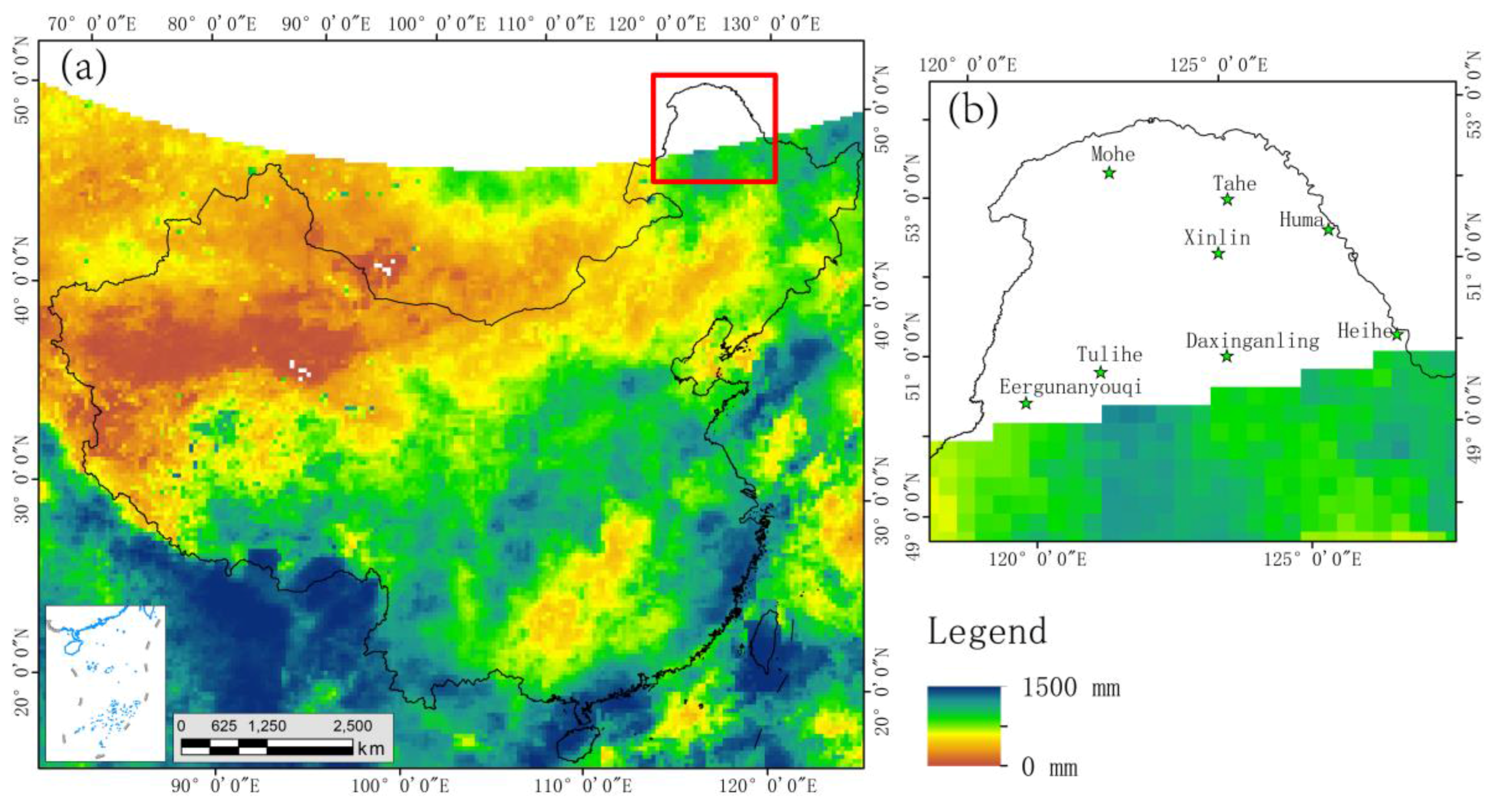
Figure 2.
Boxplots of determination coefficient of training process by using different parameters.

Figure 3.
Reconstruction results at 25 km spatial resolution: (a) reconstructed precipitation for June 2009 by using support vector machine (SVM); (b) reconstructed precipitation for June 2009 by using RF; (c) reconstructed precipitation for September 2009 by using SVM; (d) reconstructed precipitation for September 2009 by using random forests (RF).

Figure 4.
Reconstruction results at 1 km spatial resolution: (a) reconstructed precipitation for June 2009 by using SVM; (b) reconstructed precipitation for June 2009 by using RF; (c) reconstructed precipitation for September 2009 by using SVM; (d) reconstructed precipitation for September 2009 by using RF.
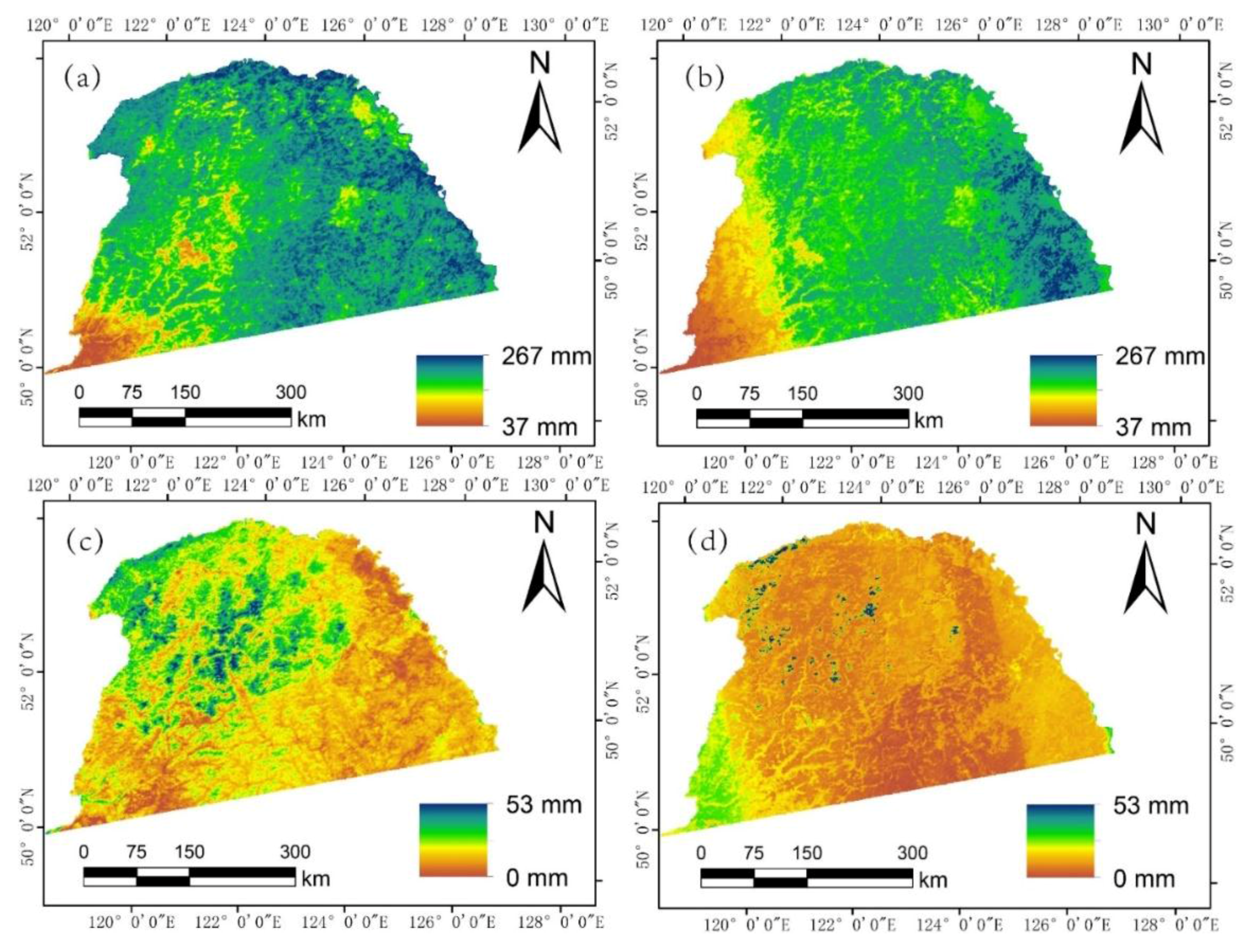
Figure 5.
Scatter plots between observed monthly total precipitation and estimated results using (a) SVM and (b) RF at spatial resolution of 25 km.
Figure 5.
Scatter plots between observed monthly total precipitation and estimated results using (a) SVM and (b) RF at spatial resolution of 25 km.
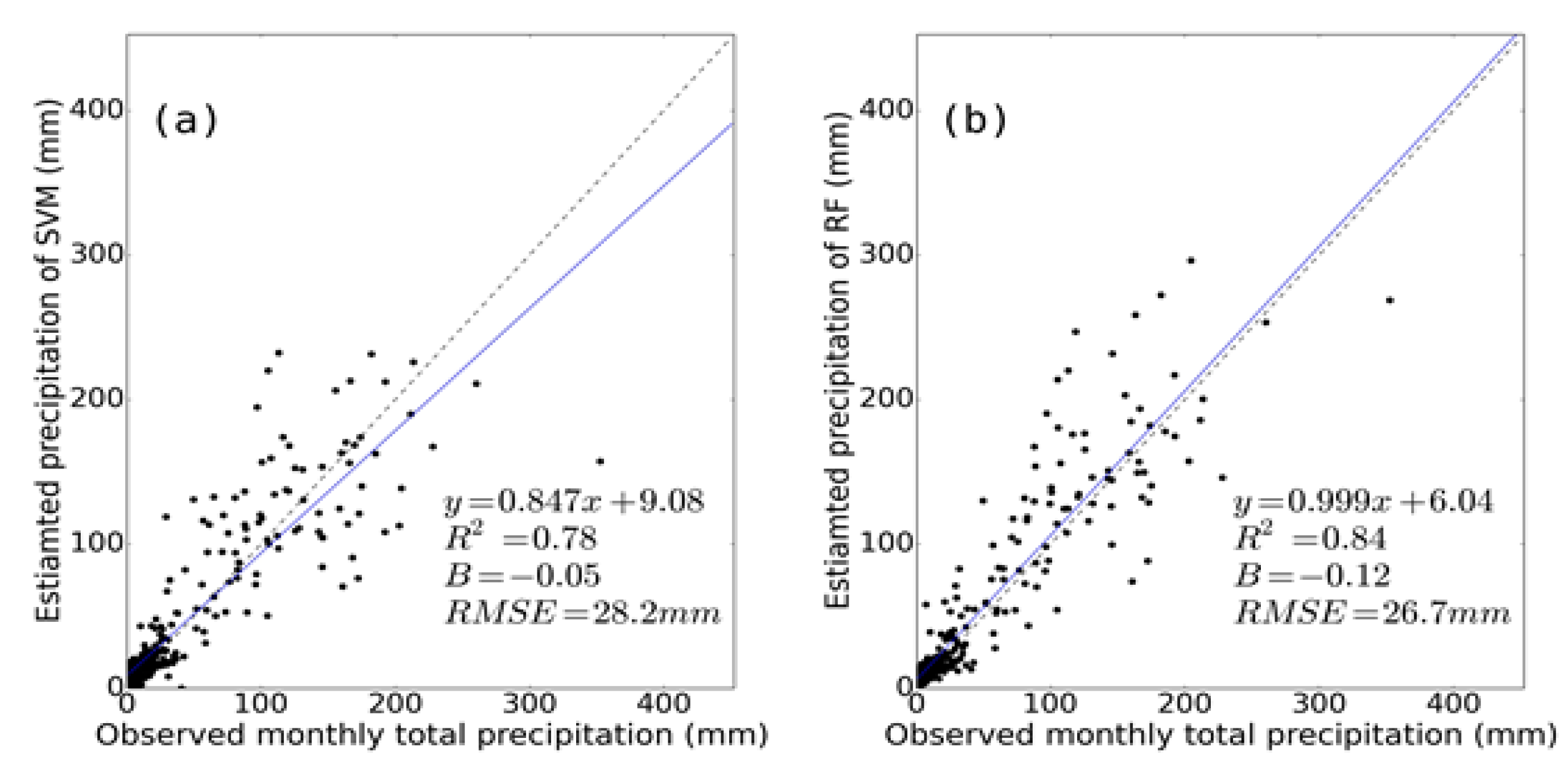
Figure 6.
Scatter plots between observed monthly total precipitation and estimated results using (a) SVM and (b) RF at spatial resolution of 1 km.
Figure 6.
Scatter plots between observed monthly total precipitation and estimated results using (a) SVM and (b) RF at spatial resolution of 1 km.

Figure 7.
Comparison of in situ observations and reconstructed monthly precipitation by using RF and SVM at eight stations, respectively.
Figure 7.
Comparison of in situ observations and reconstructed monthly precipitation by using RF and SVM at eight stations, respectively.

Figure 8.
Scatter plots between average mean absolute error (MAE) of reconstructed precipitation for each station and average precipitation observations of the stations: (a) SVM; (b) RF.
Figure 8.
Scatter plots between average mean absolute error (MAE) of reconstructed precipitation for each station and average precipitation observations of the stations: (a) SVM; (b) RF.
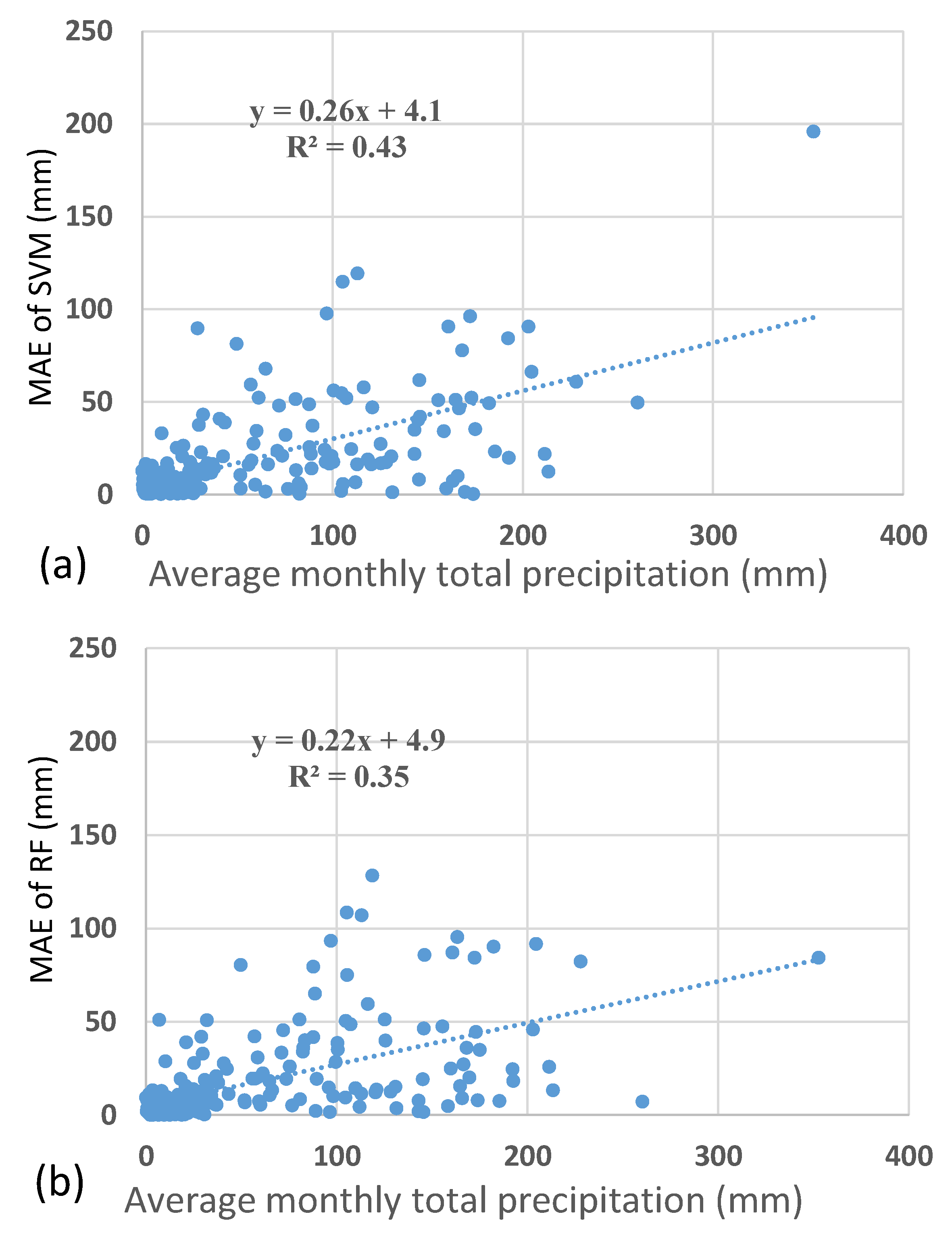
Figure 9.
(a) The R2 achieved by using SVM on different scale from January to December; (b) the R2 achieved by using RF on different scale from January to December; (c) The MAE achieved by using SVM on different scale from January to December; (d) The MAE achieved by using RF on different scale from January to December.
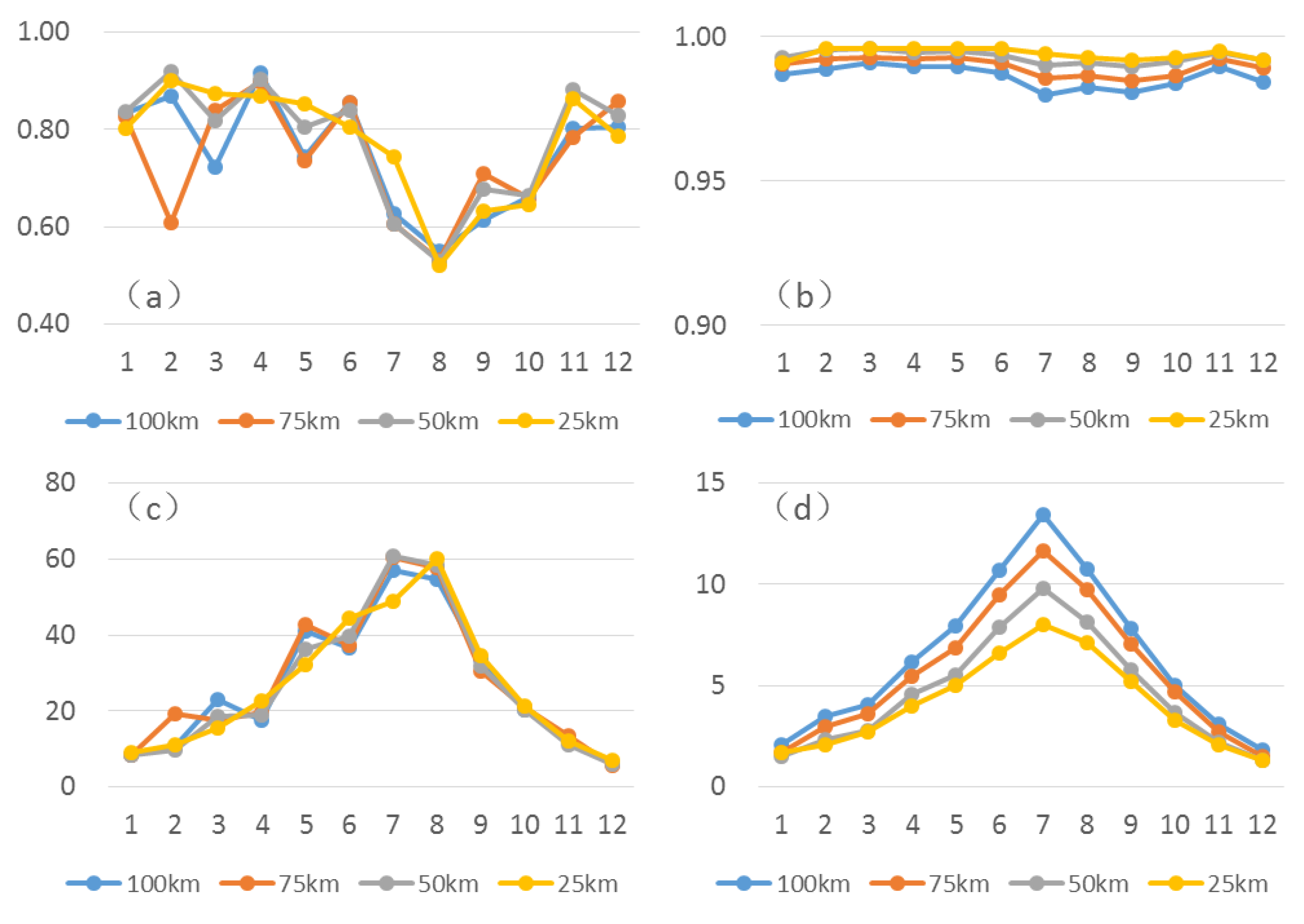
Figure 10.
Comparison of in situ observed precipitation and normalized difference vegetation index (NDVI) values at eight stations, respectively.
Figure 10.
Comparison of in situ observed precipitation and normalized difference vegetation index (NDVI) values at eight stations, respectively.

Figure 11.
Comparison of in situ observed precipitation, daytime land surface temperature (LST), and nighttime LST values at eight stations, respectively.
Figure 11.
Comparison of in situ observed precipitation, daytime land surface temperature (LST), and nighttime LST values at eight stations, respectively.


Table 1.
Parameter combinations for each algorithm.
| Algorithm | Parameter Type | Parameters |
|---|---|---|
| Support Vectors Machine | Kernel | rbf |
| Cost(C) | 20, 40, 60,80,100, 150, 200, 220, 250, 280,300 | |
| gamma | 2−6, 2−5, 2−4, 2−3, 2−2, 2−1, 1, 21, 22, 23, 24, 25, 26 | |
| Random Forests | n_estimators | 20, 40, 60, 80, 100, 120, 140, 160, 180, 200 |
Table 2.
The averaged training accuracy for different months by using the two algorithms.
| Month | SVM | RF | ||||
|---|---|---|---|---|---|---|
| R2 | MAE (mm) | RMSE (mm) | R2 | MAE (mm) | RMSE (mm) | |
| January | 0.803 | 4.2 | 8.9 | 0.991 | 0.7 | 1.7 |
| February | 0.901 | 5.1 | 11.0 | 0.996 | 1.0 | 2.1 |
| March | 0.875 | 7.5 | 15.5 | 0.996 | 1.4 | 2.7 |
| April | 0.870 | 11.8 | 22.6 | 0.996 | 2.2 | 4.0 |
| May | 0.853 | 17.8 | 32.1 | 0.996 | 2.9 | 5.0 |
| June | 0.806 | 25.7 | 44.3 | 0.996 | 3.9 | 6.6 |
| July | 0.743 | 30.0 | 49.0 | 0.994 | 5.0 | 8.0 |
| August | 0.522 | 36.5 | 60.0 | 0.993 | 4.2 | 7.1 |
| September | 0.633 | 19.9 | 34.5 | 0.992 | 3.1 | 5.2 |
| October | 0.647 | 9.9 | 21.4 | 0.993 | 1.8 | 3.3 |
| November | 0.863 | 6.2 | 12.1 | 0.995 | 1.1 | 2.1 |
| December | 0.786 | 3.4 | 7.0 | 0.992 | 0.6 | 1.3 |
| Average | 0.775 | 14.8 | 26.5 | 0.994 | 2.3 | 4.1 |
Table 3.
The correlation coefficient, root mean squared error (RMSE), and Bias between observed and estimated monthly precipitation of 25 km resolution at eight stations.
Table 3.
The correlation coefficient, root mean squared error (RMSE), and Bias between observed and estimated monthly precipitation of 25 km resolution at eight stations.
| Station | R2 | RMSE (mm) | B | |||
|---|---|---|---|---|---|---|
| SVM | RF | SVM | RF | SVM | RF | |
| Mohe | 0.66 | 0.72 | 32.53 | 31.30 | −0.02 | −0.09 |
| Tahe | 0.71 | 0.76 | 34.59 | 31.87 | −0.11 | −0.12 |
| Xinlin | 0.85 | 0.89 | 24.96 | 21.60 | 0.06 | 0.01 |
| Huma | 0.83 | 0.88 | 28.52 | 38.38 | −0.17 | −0.28 |
| Eergunayouqi | 0.88 | 0.92 | 16.54 | 13.67 | −0.19 | −0.18 |
| Tulihe | 0.86 | 0.93 | 21.80 | 21.13 | −0.16 | −0.18 |
| Daxinganling | 0.86 | 0.91 | 23.63 | 19.29 | 0.01 | −0.03 |
| Heihe | 0.86 | 0.90 | 37.20 | 27.23 | 0.16 | −0.07 |
Table 4.
The correlation coefficient, RMSE, and Bias between observed and estimated monthly precipitation of 1 km resolution at eight stations.
Table 4.
The correlation coefficient, RMSE, and Bias between observed and estimated monthly precipitation of 1 km resolution at eight stations.
| Station | R2 | RMSE (mm) | B | |||
|---|---|---|---|---|---|---|
| SVM | RF | SVM | RF | SVM | RF | |
| Mohe | 0.66 | 0.72 | 32.53 | 31.30 | −0.02 | −0.09 |
| Tahe | 0.71 | 0.76 | 34.59 | 31.87 | −0.11 | −0.12 |
| Xinlin | 0.85 | 0.89 | 24.96 | 21.60 | 0.06 | 0.01 |
| Huma | 0.83 | 0.88 | 28.52 | 38.38 | −0.17 | −0.28 |
| Eergunayouqi | 0.88 | 0.92 | 16.54 | 13.67 | −0.19 | −0.18 |
| Tulihe | 0.86 | 0.93 | 21.80 | 21.13 | −0.16 | −0.18 |
| Daxinganling | 0.86 | 0.91 | 23.63 | 19.29 | 0.01 | −0.03 |
| Heihe | 0.86 | 0.90 | 37.20 | 27.23 | 0.16 | −0.07 |
© 2017 by the authors. Licensee MDPI, Basel, Switzerland. This article is an open access article distributed under the terms and conditions of the Creative Commons Attribution (CC BY) license (http://creativecommons.org/licenses/by/4.0/).
Share and Cite
MDPI and ACS Style
Jing, W.; Zhang, P.; Jiang, H.; Zhao, X. Reconstructing Satellite-Based Monthly Precipitation over Northeast China Using Machine Learning Algorithms. Remote Sens. 2017, 9, 781. https://doi.org/10.3390/rs9080781
AMA Style
Jing W, Zhang P, Jiang H, Zhao X. Reconstructing Satellite-Based Monthly Precipitation over Northeast China Using Machine Learning Algorithms. Remote Sensing. 2017; 9(8):781. https://doi.org/10.3390/rs9080781
Chicago/Turabian StyleJing, Wenlong, Pengyan Zhang, Hao Jiang, and Xiaodan Zhao. 2017. "Reconstructing Satellite-Based Monthly Precipitation over Northeast China Using Machine Learning Algorithms" Remote Sensing 9, no. 8: 781. https://doi.org/10.3390/rs9080781
Note that from the first issue of 2016, this journal uses article numbers instead of page numbers. See further details here.