Radiometric Cross-Calibration of GF-4 PMS Sensor Based on Assimilation of Landsat-8 OLI Images


1
State Key Laboratory of Information Engineering in Surveying, Mapping and Remote Sensing, Wuhan University, Wuhan 430079, China
2
Department of Geographical Sciences, University of Maryland, College Park, MD 20742, USA
*
Author to whom correspondence should be addressed.
Remote Sens. 2017, 9(8), 811; https://doi.org/10.3390/rs9080811
Submission received: 23 April 2017
/
Revised: 29 July 2017
/
Accepted: 4 August 2017
/
Published: 9 August 2017
Abstract
:Earth observation data obtained from remote sensors must undergo radiometric calibration before use in quantitative applications. However, the large view angles of the panchromatic multispectral sensor (PMS) aboard the GF-4 satellite pose challenges for cross-calibration due to the effects of atmospheric radiation transfer and the bidirectional reflectance distribution function (BRDF). To address this problem, this paper introduces a novel cross-calibration method based on data assimilation considering cross-calibration as an optimal approximation problem. The GF-4 PMS was cross-calibrated with the well-calibrated Landsat-8 Operational Land Imager (OLI) as the reference sensor. In order to correct unequal bidirectional reflection effects, an adjustment factor for the BRDF was established, making complex models unnecessary. The proposed method employed the Shuffled Complex Evolution-University of Arizona (SCE-UA) algorithm to find the optimal calibration coefficients and BRDF adjustment factor through an iterative process. The validation results revealed a surface reflectance error of <5% for the new cross-calibration coefficients. The accuracy of calibration coefficients were significantly improved when compared to the officially published coefficients as well as those derived using conventional methods. The uncertainty produced by the proposed method was less than 7%, meeting the demands for future quantitative applications and research. This method is also applicable to other sensors with large view angles.
1. Introduction
China began implementation of a high-definition earth observation system (HDREOS) in 2010 as a step towards an all-weather, all-day earth observation network with global coverage. As an important part of the system, the GF-4, launched on 29 December 2015, is the first Chinese optical remote sensing satellite in geostationary orbit designed specifically for civil use. A panchromatic multispectral sensor (PMS) sensor is onboard the GF-4 satellite, providing images for about one third of the earth at a high spatial resolution (50 m) and wide coverage (500 km). It can not only adjust to the observation area within a few minutes, but also achieves up-to-the-minute high-frequency continuous imaging of the same area. In the first operating year, the GF-4 PMS played an important role in many applications including monitoring a forest fire in Diebu city Gansu province, China and the Nepartak typhoon (http://www.cresda.com/CN/xwzx/xwdt/index.shtml).
Accurate radiometric calibration is a prerequisite for quantitative applications of the GF-4 PMS. Vicarious calibration and cross-calibration are commonly used on-orbit calibration techniques [1,2,3,4,5]. The China Center for Resources Satellite Data and Application (CCRSDA) used the vicarious calibration technique to calibrate the GF-4 PMS at the Dunhuang calibration site, and published the radiometric calibration coefficients on its official website (http://www.cresda.com/CN/Downloads/dbcs/10506.shtml). However, uncertainty in the official coefficients has not been verified by any other reports or studies. Vicarious calibration is time-consuming, expensive, and labor intensive because of the strict requirements of synchronous field measurements. Furthermore, it cannot be used to calibrate historical sensor data [6]. Cross-calibration is another important method, based on a reference sensor without synchronous surface observations. The accuracy of the cross-calibration method could be as high as that of the vicarious calibration technique, with much lower cost and at a higher frequency. Cross-calibration can be used for historical images. Thus, cross-calibration is an alternative way to radiometrically calibrate GF-4 PMS with high accuracy and low cost.
Cross-calibration has been applied to optical sensors with small view angles, but rarely to sensors with large view angles. Mishra et al. used cross-calibration techniques to evaluate the radiometric consistency between Landsat-8 Operational Land Imager (OLI) and Landsat 7 Enhanced Thematic Mapper Plus (ETM+) over the Libya 4 pseudo invariant calibration site [7]. Gao et al. used a simple cross-calibration method named spectrum matching (SM) to cross-calibrate the GF-1 PMS with the Landsat-8 OLI and MODIS (Moderate-Resolution Imaging Spectroradiometer) as the reference sensors, and the Landsat-8 OLI yielded more accurate calibration coefficients than those estimated by the MODIS [6]. Li et al. cross-calibrated GF-1 WFV (Wide Field of View) using an image-based cross-calibration method with respect to the Landsat-8 OLI [8]. Most previous studies calibrated a target sensor using a reference sensor both with small view angles and considered the Top of Atmosphere (TOA) radiance or reflectance of the two sensor data are equal without Atmospheric Correction or bidirectional reflectance distribution function (BRDF) correction. It is unnecessary to consider the unequal effects of atmospheric radiation transfer and BRDF between the two sensors when calibrating a target sensor, as these effects are approximately the same when using simultaneous image pairs. However, for cross-calibrating the target sensor (GF-4 PMS) with a large view angle against the reference sensor (Landsat-8 OLI) with a narrow view angle, these issues may add error to the cross-calibration coefficients, because the atmospheric radiation transfer and BRDF are both closely related to view angles [9,10,11,12]. Angal et al. and Feng et al. used the semi-empirical kernel function model with the aid of MODIS BRDF products to eliminate the BRDF effects [13,14]. Yang et al. retrieved the BRDF parameters of the GF-1 WFV and GF-4 PMS data using the BRDF characterization of the calibration site fitted by the Landsat-8/OLI data and the digital elevation model (DEM) derived by the ZY-3 three-line camera data (TLC) [15,16]. These methods are complex and may produce new errors due to the significant differences in spatial resolution between the MODIS BRDF or the DEM products and the GF-4 PMS.
In this paper, we propose a novel and simple cross-calibration method based on data assimilation for sensors with large view angles. The proposed method was implemented to cross-calibrate GF-4 PMS with Landsat-8 OLI at the Dunhuang calibration site, China. The Landsat-8 OLI is one of the most commonly used reference sensors for cross-calibration [17], with uncertainties in calibration as low as 3% for reflectance and 5% for radiance [18]. We considered cross-calibration as an optimal approximation problem and introduced data assimilation techniques into this process. A BRDF adjustment factor was established to correct the unequal bidirectional effects, making complex models unnecessary. The Shuffled Complex Evolution-University of Arizona (SCE-UA) algorithm determined the optimal calibration coefficients and BRDF adjustment factor, through an iterative process.
The rest of this paper is as follows: Section 2 summarizes the characteristics of test sites, satellites and data sets, followed by the cross-calibration method in Section 3. Section 4 presents cross-calibration and validation results from the proposed method and a comparison of these results to RTM-BRDF and SM methods, as well as officially provided coefficients. The uncertainties of the proposed method are detailed in this section. Section 5 discusses the results of the proposed method and possible applications in the future.
2. Calibration Sites and Data Sets
2.1. Calibration Sites
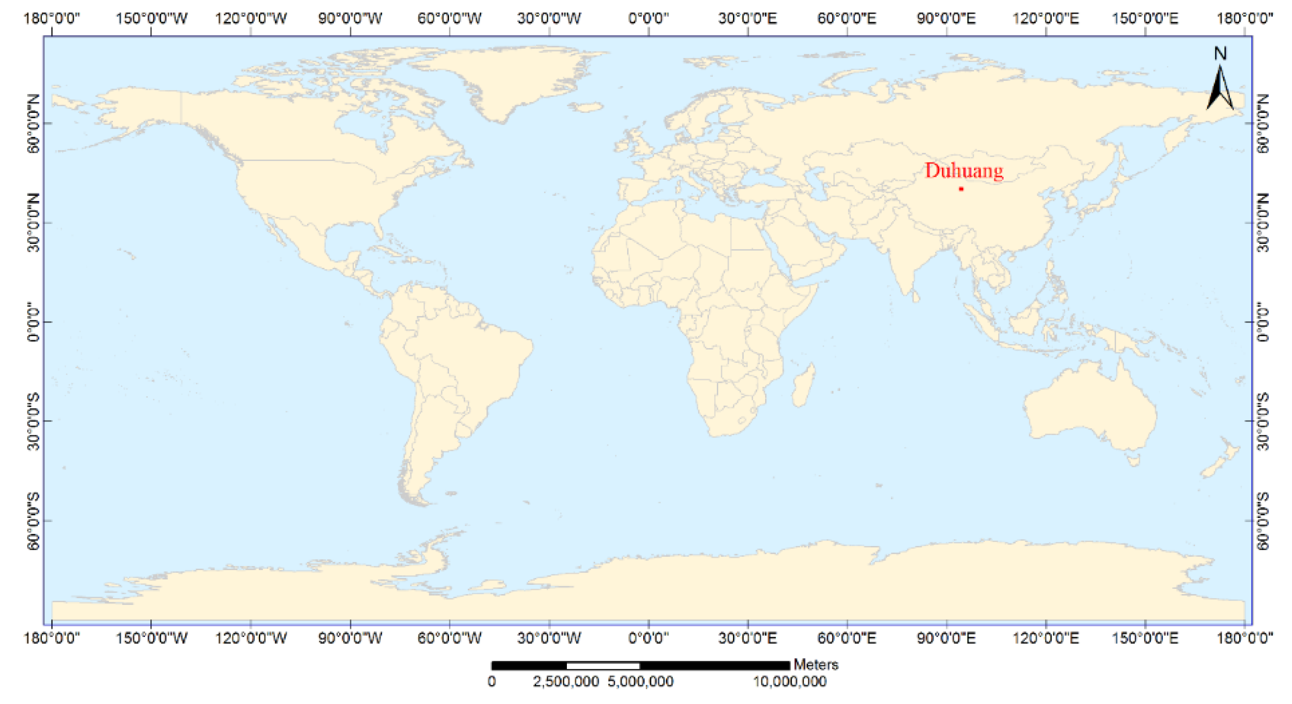
The Dunhuang calibration site is the test site used in our research; it is China’s first on-orbit calibration site for visible/near infrared (NIR) sensors. The site is located 70 km southwest of Dunhuang city, Gansu province, China, has the geographic coordinates 40°05′N–40°25’N, 94°24’E–94°40’E, and is at an elevation of about 1160 m above sea level. Situated in a desert alluvial fan, it has a uniform area of 10 km × 10 km with the radiometric spatial uniformity of 2% coefficient of variation (CV) and temporal stability of about 3% CV [19]. The surface of the ground is homogeneous and flat, composed of small black stones, sand, and clay with no vegetation. According to data from the Dunhuang Meteorological Bureau, the site typically has 112 clear-sky days and 288 days with a visibility ≥10 km, indicating that there is low probability of interference from aerosols, water vapor, and clouds at the Dunhuang test site. In addition, the surface reflectance spectrum is in the middle part of the dynamic range of the optical satellite remote sensors and is relatively stable [19]. Therefore, the Dunhuang calibration site has been widely used for calibrating many sensors such as the CBERS-02/CCD, FY-3A/MERIS, and HJ-1A, 1B/CCD [3,20,21].
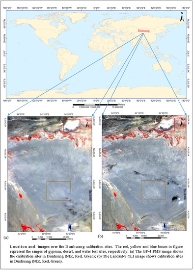
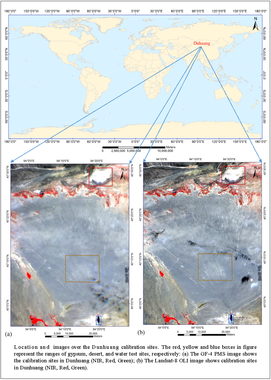
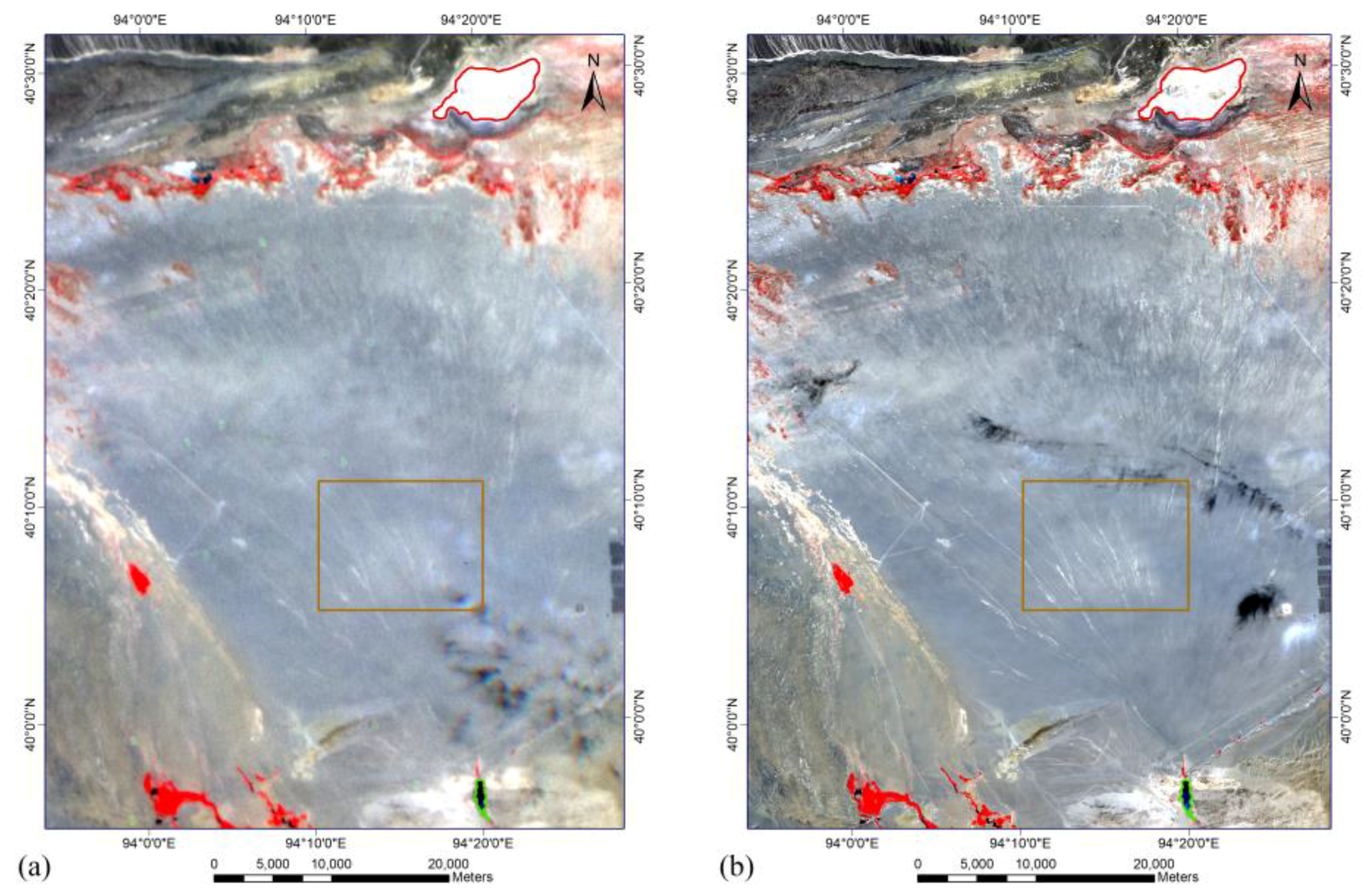
To collect samples with reflectance from low to high, in addition to the main site, samples were collected from the highly reflective gypsum located 20 km north of the desert field and from the lowly reflective water targets; these were used as additional test sites for cross-calibration (see in Figure 1). The historical measured data show that: these three sites have stable surface reflectance and their relative differences of the spectral reflectance within the range of 350–1000 nm are all less than 1% [22].
2.2. Data Sets
Two sets of data obtained on different dates were employed in the experiment, one from the Dunhuang test site for cross-calibration and another for validation from Wuhan and Yunnan in China. Both consist of GF-4 PMS and Landasat-8 OLI image pairs with minimal cloud coverage acquired on the same day. The quality assessment band of Landsat-8 OLI image is used to eliminate cloud and snow pixels to make sure the samples are valid (https://landsat.usgs.gov/qualityband). Figure 2 shows the GF-4 PMS and Landsat-8 OLI images over the calibration sites in Dunhuang. The spectral responses of Landsat-8 OLI and GF-4 PMS were compared and analyzed, as shown in Figure 3. The response spectrums of GF-4 PMS are wider than response spectrums from the Landsat-8 OLI, especially in the NIR band. The sensor parameters of the GF-4 PMS and Landsat-8 OLI are summarized in Table 1. As seen in the table, the view angles and swath of the GF-4 PMS are quite different from that of the Landsat-8 OLI. Thus, the bidirectional reflectance effects due to differences in illumination and observation angles are significant and cannot be neglected.
MODIS aerosol products were used to obtain the input atmospheric parameters for the 6S atmospheric correction model, such as aerosol optical thickness (AOT) and aerosol type. The MODIS aerosol products provide daily global data at a spatial resolution of 1 km, and can be freely downloaded from NASA website. Quality assurance (QA) flags in the aerosol data are provided to describe the product quality and the confidence on retrieval processing. The QA flag is coded as 0 for bad, 1 for marginal, 2 for good, and 3 for very good [23]. To obtain the valid products with good quality, we chose the aerosol products with flags of 2 or 3 and apply spatial interpolation to obtain the aerosol data of the whole calibration site. The MODIS products have five aerosol types that are not identical to those used in the 6S model. In practice, the mixed or sulfate aerosol type in the MODIS corresponds to a continental or desert model in 6S [14].
The USGS spectral library (splib06, [24]) was used in this research to obtain the standard spectrums of the targets over Dunhuang calibration sites to calculate the spectral band adjustment factors (SBAF) for different sensors. The library contains over 1300 spectra including visible, near-infrared, and mid-infrared spectra. The spectral samples measured hundreds of materials, including manufactured chemicals, coatings, liquids, minerals, and plants. Thus, most features have corresponding spectrums in the library.
3. Methodology
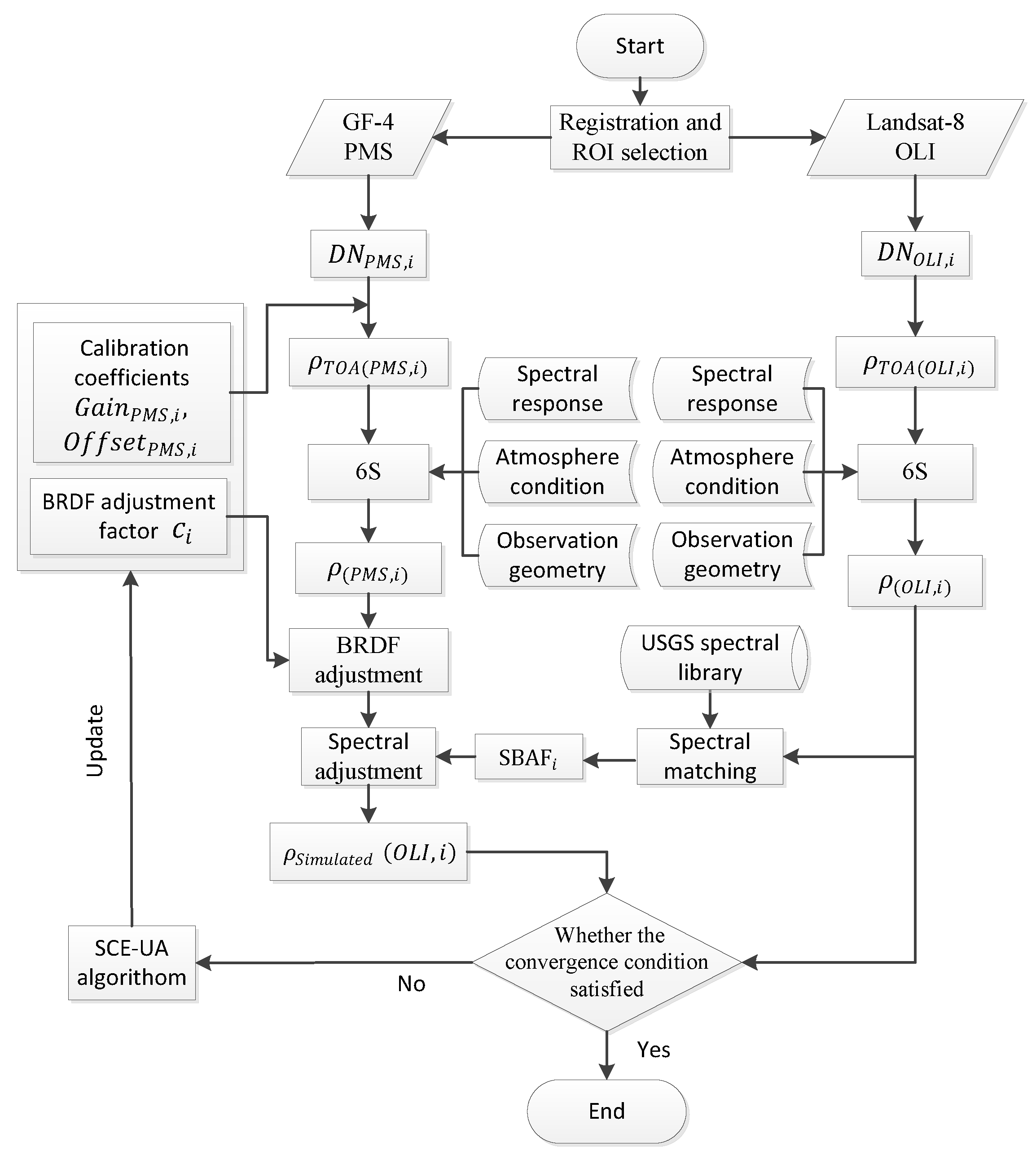
In this paper, the cross-calibration method based on data assimilation for sensor data with large-angle observation is proposed. We use the well-calibrated nadir view of Landsat-8 OLI data as reference. The surface reflectance of the Landsat-8 OLI data is first retrieved though calibration and atmospheric correction by 6S model. The SBAF is then calculated after spectral matching using USGS spectral library. Thirdly, the retrieved surface reflectance of GF-4 PMS calculated using the initial calibration coefficients is adjusted by SBAF and initial BRDF adjustment factor to simulate the surface reflectance of Landsat-8 OLI. Then the simulated surface reflectance and the retrieved surface reflectance of the Landsat-8 OLI are compared. If the difference between them is within the threshold, the calibration coefficients are obtained; otherwise search for new calibration coefficients and BRDF adjustment factor and then repeat the above steps until the convergence condition is satisfied. Finally, the cross-calibration of GF-4 PMS is performed. Figure 4 shows the cross-calibration process in this study and we discuss the major steps below in detail. The shorter notations in the flow chart refer to the descriptions in Section 3.1, Section 3.2 and Section 3.3.
3.1. TOA Reflectance Calculation
Radiometric calibration converts the digital number (DN) value into the radiance value of the corresponding pixel to eliminate the system error from the sensor. Radiance often responds linearly to the quantified standard DNs. Thus, for a given band of GF-4 PMS data, the relationship between the TOA radiance and the image digital number can be written as follows:
where is the converted radiance () is the band-specific multiplicative rescaling gain and is the band-specific additive bias. Then the radiance value can be converted into TOA reflectance by the following formula:
where is the TOA reflectance of band ; is the solar zenith angle and is the distance between the sun and the earth in astronomical units; is the average exo-atmosphere solar spectral irradiance (), the formula to calculate the value is as follows:
where is the continuous exo-atmospheric solar spectral irradiance (), obtained by the Thuilier solar spectral irradiance model [25]; and is the normalized spectral response function of the band .
The TOA reflectance of the GF-4 PMS data can be obtained using Equations (1)–(3), and that of the Landsat-8 OLI data can be calculated using reflectance scaling coefficients provided by the metadata file:
where is the band-specific multiplicative rescaling factor, and is the band-specific addictive rescaling factor obtained from the metadata. is the quantized standard pixel value of Landsat-8 OLI product, and is the sun elevation angle from the metadata.
3.2. Atmospheric Correction, Spectral and BRDF Adjustment and Simulation
The disparities in surface reflectance between the GF-4 PMS and Landsat-8 OLI are caused by three factors. These include the difference in atmospheric radiation transfer process due to satellite elevation and observation angle that leads to different atmospheric radiation transfer paths in both distance and direction; the difference in the BRDF due to the effects of viewing and illumination angles; and the different spectral responses of the two sensors.
At the Dunhuang calibration site, there is a large gap between the sensor zenith angle of GF-4 PMS (49.77°) and that of the Landsat-8 OLI (0°), as well as the sensor azimuth angle (see in Table 2). The influence of atmosphere due to viewing angle will increase the uncertainty of cross-calibration. Moreover, the large zenith angle has a significant influence on BRDF. Therefore, in order to obtain accurate cross-calibration coefficients, problems related to the large view angle must be solved.
The incoming signal received by the satellite sensor contains reflection from the surface and reflection from the atmosphere. Assuming a standard Lambertian surface, the formula for the TOA reflectance is as follows [26]:
where and are solar zenith angle and azimuth angles respectively; and are satellite zenith angle and azimuth angles, respectively; is the atmospheric spherical albedo; and are the downward and upward transmittances; is the reflectance from the atmosphere, and is the surface reflectance.
According to the Equation (6) to obtain the surface reflectance, the values of the , and are required. The 6S model estimates these parameters from known observation geometry, atmospheric condition, and spectral response functions. In our research, MODIS AOT data were used here to get the aerosol optical depth and aerosol type. The BDRF was considered separately in the following steps, assuming no bidirectional reflection effects during atmosphere correction. The input parameters in the 6S model for one image pair are listed in Table 2.
The reflection from the surface of the earth under natural conditions is bidirectional; the intensity of reflected irradiance depends on the direction of incident radiance and the reflection direction, and usually described by the BRDF [27]. The BRDF is defined as the ratio of the reflected radiance from the target surface in the directions of and to the incident irradiance along the directions of and :
where B is the BRDF; and stand for the solar zenith angle and azimuth angle; and stand for the viewing zenith angle and azimuth angle.
There are several typical BRDF models that can describe the anisotropic fractures of the surface reflection, such as the Ross- Li BRDF model [28,29], the Rahman BRDF model [30], and the Staylor–Suttles BRDF model [31]. The BRDF model is quite complex. To obtain the unknown constant coefficients in the model, MODIS BRDF products or field measurements are required, resulting labor intensive, high cost and potential errors to cross-calibration because of large differences in spatial resolution and spectral response. Thus, a BRDF adjustment factor was established to eliminate the difference in the surface reflectance between the GF-4 PMS and Landsat-8 OLI due to the differences in viewing and illumination angles. For band , the BRDF adjustment factor can be described as follows [32]:
where is the BRDF of the GF-4 PMS, and is the BRDF of the Landsat-8 OLI; and are the solar zenith angle and azimuth angle of the GF-4 PMS; and are the viewing zenith angle and azimuth angle of the GF-4 PMS; and are the solar zenith angle and azimuth angle of the Landsat-8 OLI; and are the viewing zenith angle and azimuth angle of the Landsat-8 OLI.
The definition of the BRDF adjustment factor in Equation (7) is to describe the physical meaning of the factor which make BRDF correction using the factor reasonable. We do not calculate directly in this way. As mentioned before, BRDF model is complex and difficult to estimate duo to the requirement of extra data or measurements. Thus, we use the assimilation algorithm to obtain the optimal value of , instead of calculate the BRDF of the GF-4 PMS and the Landsat-8 OLI through complex model.
A BRDF adjustment factor was established to eliminate the BRDF effect between the GF-4 PMS and Landsat-8 OLI due to the differences in viewing and illumination angles can be estimated. Thus, the surface reflectance of GF-4 PMS image acquired from its angles can be converted to the surface reflectance observed from the illumination and viewing angles of Landsat-8 OLI image, using Equations (8) as follows:
where represents the surface reflectance; and are the solar zenith angle and azimuth angle of the GF-4 PMS; and are the sensor zenith angle and azimuth angle of the GF-4 PMS; and are solar viewing zenith angle and azimuth angle of the Landsat-8 OLI; and are sensor zenith angle and azimuth angle of the Landsat-8 OLI. The difference between the spectral response of the target sensor and that of the reference sensor is eliminated by the SBAF. The formula of SBAF is as follows [33]:
where is the spectral band adjustment factor for band ; and are respectively the surface reflectance of GF-4 PMS and Landsat-8 OLI; is the continuous spectral reflectance of the target, and is the continuous exo-atmospheric solar spectral irradiance; and are the spectral response function of GF-4 PMS and Landsat-8 OLI, respectively; and , and , are respectively the wavelength range of GF-4 PMS and Landsat-8 OLI for specific band. Then the surface reflectance of Landsat-8 OLI can be simulated as:
The reflectance of various targets is different, as is the spectral band adjustment factor, thus, it is difficult to obtain the reflectance of each ROI through measurement or by using a hyper-spectral image. The test sites at Dunhuang however, have simple types of ground targets and corresponding reflectance curves are easily obtained from the existing USGS spectral library. The 6s model was used for atmospheric correction of Landsat-8 OLI image to get discrete surface reflectance of the ROIs. Best match spectral curves can be found in the USGS spectral library. We plugged them into the Equation (9), and then calculated the SBAF. For gypsum target, the differences between the atmospherically corrected Landsat-8 OLI reflectance and the gypsum spectral curves in the USGS spectral library are quite large. Fortunately, the CCRSDA provides the filed measured spectrum of the gypsum in Dunhuang (http://218.247.138.119/CN/fwyyytx/zgwxdbjx/5368.shtml). The measured spectrum of gypsum matched well with the mean reflectance of Landsat-8 OLI. We used the spectrum to calculate the SBAF for gypsum case. The results of spectral matching can be seen in Figure 5.
After the atmospheric correction by the 6S model of the GF-4 PMS images, the following formula simulates the surface reflectance of Landsat-8 OLI images:
where is the simulated surface reflectance of a Landsat-8 OLI image; and is the atmospherically corrected surface reflectance of a GF-4 PMS image.
3.3. The SCE-UA Algorithm
SCE-UA algorithm is a global optimization algorithm proposed by Duan in 1993 [34]. This algorithm was originally developed for hydrological models. We applied it to cross-calibration. The idea of complex shape segmentation and mixing introduced in this algorithm improves search efficiency, computation speed, and global search ability. SCE-UA is not sensitive to the initial values of the optimization parameters, thus avoiding excessive reliance on prior knowledge during optimization process and solves the problems caused by missing initial parameter values [35]. Research shows that SCE-UA can converge to the global optimal solution efficiently due to its fast convergence speed and good stability [36]. Although SCE-UA algorithm has many parameters, most can take default values [37]. The objective function used in our research is as follows:
where is the simulated surface reflectance of a Landsat-8 OLI image; and is the atmospherically corrected surface reflectance of a Landsat-8 OLI image.
To ensure the feasibility of the optimization algorithm and the reliability of the results, for each ROI, SCE_UA algorithm runs independently 100 times. The initial values of the optimized parameters are random values within a defined range. The optimization process ends when one of the following three conditions is encountered: (1) the CV of the continuous five optimal values of objective function is less than 0.001; (2) the objective function is calculated more than 10,000 times; (3) The value of an optimized parameter shrinks to a predetermined range. If the optimization process ends in the first case, the optimization was successful, the radiometric calibration coefficients and BRDF adjustment factors corresponding to the minimum objective function values are the optimal results. If otherwise, the optimization process has failed. In this study, the success rate was 100%.
3.4. Cross-Calibration
As shown in Figure, the steps of cross-calibration are summarized as follows:
- Geometrically register the GF-4 PMS and reference Landsat-8 OLI images with error controlled to within one pixel. Select regions of interest (ROI) as presented in Li et al. [8].
- Calculate the TOA reflectance in the Landsat-8 OLI image using Equations (4). Then perform atmospheric correction to obtain the surface reflectance of ROIs in the Landsat-8 OLI image , immediately after the registration and ROIs selection step.
- Perform Spectral matching to get the optimal spectra from the USGS spectral library to calculate between GF-4 PMS and Landsat-8 OLI by Equation (9). Use the minimum Mahalanobis distance between the Landsat-8 OLI surface reflectance and the spectra in USGS library to determine the best-matching spectra.
- Initialize the calibration coefficients and of GF-4 PMS and BDRF adjustment factor . Then use the initial values to calculate the TOA reflectance of GF-4 PMS data using Equations (1)–(3) and derive the surface reflectance using the 6S atmospheric correction model . The simulated surface reflectance of Landsat-8 OLI is obtained using Equation (11).
- Compare the Landsat-8 OLI simulated surface reflectance and the retrieved reflectance . If the difference between them is small enough to satisfy the convergence condition, then the optimal calibration coefficients and BDRF adjustment factor are obtained. If the opposite happens, the SCE-UA optimization algorithm is used to update the values of , , and to calculate a new Landsat-8 OLI simulated surface reflectance . Perform the same loop iteration, until reaching the termination condition.
4. Experimental Results and Analysis
4.1. Cross-Calibration Results
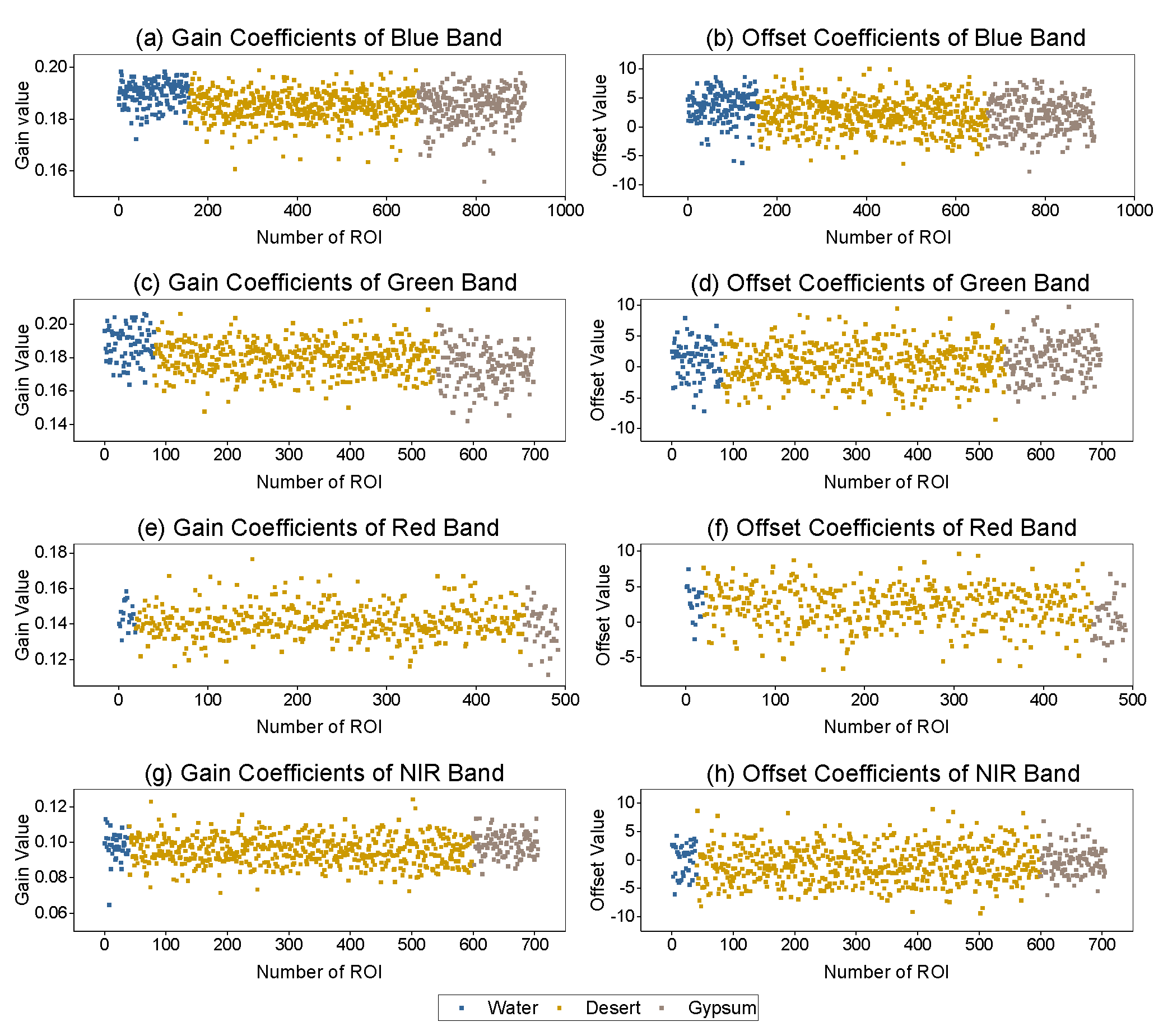
The radiometric calibration coefficients of the GF-4 PMS were calculated using the proposed method, based on the selected ROIs in the high reflective gypsum, medium reflective desert, and low reflective water test sites. Figure 6 shows the gain and offset coefficients of all ROIs for each band. In the figure, each point represents a ROI. For each band, the degree of consistency in the ordinate values of the points indicates the quality of the results.
As seen in Figure 6, the sampling ROIs of each band are greater than or equal to 500. The gain coefficients of each band are quite consistent except for very few ROIs with relatively larger errors. Among the four bands, the red band has the least sampled ROIs, and the calculated gain values are more dispersed than the other three bands. The offset coefficients of the four bands are more dispersed, especially the green and red bands.
The statistical analysis of the obtained cross-calibration coefficients is shown in Table 3. The CV is the variation coefficient, which represents the degree of dispersion in the data. The minimum, maximum and mean values of the coefficients of all the ROIs in each band are also listed.
As shown in Table 3, the mean of gains and offsets for gypsum, desert and water case are quite similar, and the gain coefficients for the four bands all vary within a small range with small differences between the maximum and the minimum. The largest CV is only 6.43% of red band, which indicates that the proposed method is feasible, and the calculation results are effective. The disparities between the maximum value and the minimum value of offset coefficients are much larger than those of the gain coefficients for each band, so as to the CV. It can be explained by the fact that the effective range of the offset coefficient (−30–30) is much larger than that of the gain coefficient (0–1). The CV of offset coefficients however, are more than 100% for three bands, especially the green band, up to 229.24%.
Thus, it is not reasonable to take the mean offset value of ROIs as the offset coefficient for a specific band. Fortunately, the radiance is not sensitive to the change of gain coefficient. Furthermore, the gain and offset coefficients of each ROI are not completely independent but one to one correspondence because they are a set of optimal solutions obtained by the assimilation algorithm. Thus, the gain coefficient can be first determined by taking the mean as the gain coefficient of the band after eliminating very few ROIs that are 10% larger or smaller than the mean, and then the offset coefficient is obtained according to the corresponding relation between the gain and offset coefficients.
The calibration coefficients of four bands derived by three different cross-calibration methods are shown in Table 4 and the officially provided coefficients are listed. In order to evaluate the reliability of the RTM-DA method, based on the same sampling ROIs, SM and RTM-BRDF methods are used to calculate the calibration coefficients. The SM method cross-calibrates target sensor based on spectral matching without atmosphere correction and BRDF correction [8]. The RTM-BRDF method is based on radiative transfer model (RTM) with BRDF correction and simulation proposed in Feng et al. [14] The RTM-DA is the cross-calibration method based on RTM with BRDF corrected by using data assimilation algorithm proposed in this paper. The official calibration coefficients are the results of vicarious calibration published by CRESDA through its website they were used for validation in Yang et al. [16]. The difference between the four versions of calibration coefficients are also summarized in Table 4. Because the officially provided coefficients do not contain the offset coefficients of GF-4 PMS, only the differences of the gain values between the four versions of coefficients are estimated.
It can be inferred from Table 4 that for the GF-4 PMS, the differences between atmospheric radiation transfer and the bidirectional reflection have a significant influence on cross-calibration. As seen in Table 4, the differences between the gain coefficients obtained by RTM-DA and those derived by SM are relatively larger, especially in the NIR band, with a difference as high as 33.36% in column D 1. In comparisons between RTM-DA and RTM-BRDF shown in column D 2, the difference rises to 21.71% for the NIR band, but the differences for the blue, green and red bands are all much smaller, 6.49%, 3.75%, and 1.26% respectively. Compared to the official gain coefficients, the gain coefficient for the green band calculated by the RTM-BRDF method is the closest to the official coefficient; the difference ratio was only 0.48%, while those of blue and NIR bands are relatively much larger as seen in column D 3. Relatively smaller differences between the RTM-BRDF and official coefficients are observed for all four spectral bands, where the differences for the blue, green and red bands are all less than 7% .In the NIR band the difference was 11.2%, column D 4. The differences in the gain coefficient for the NIR band between the four versions of the coefficients are significant, with differences of more than 10%.
4.2. Validation Results
Due to the lack of in situ measurements, Landsat-8 images were used to evaluate the calibration coefficients obtained by the proposed method. The process of simulating surface reflectance of GF-4 PMS using Landsat-8 OLI images is similar to that of cross-calibration. After atmospheric correction, BRDF adjustment, and spectral matching, the simulated radiance and surface reflectance from Landsat-8 OLI data are regarded as ground truths. For a comprehensive validation, the calibration coefficients derived through the SM and RTM-BRDF methods also participate in the comparison, along with the officially provided coefficients. The results retrieved by the four versions of coefficients are compared with the ground truths, and the accuracies were analyzed.
Figure 7 shows the distribution of the bias in radiance generated from different versions of calibration coefficients. The mean and standard deviation of the radiance biases are shown in this figure. If the points are distributed close to y = 0 line, then the corresponding method yields accurate calibration coefficients with a small radiance bias.
It can be seen from Figure 7 that the performance of RTM-BRDF method is similar to that of RTM-DA. In addition, RTM-DA and RTM-DA methods have smaller mean radiance biases than the SM method and official coefficients do, as the distribution of the biases are closer to 0 for all four bands. The calibration coefficients calculated by SM method and the official coefficients produce larger radiance biases, and the distributions of the biases are more dispersed from the mean, especially for the NIR band.
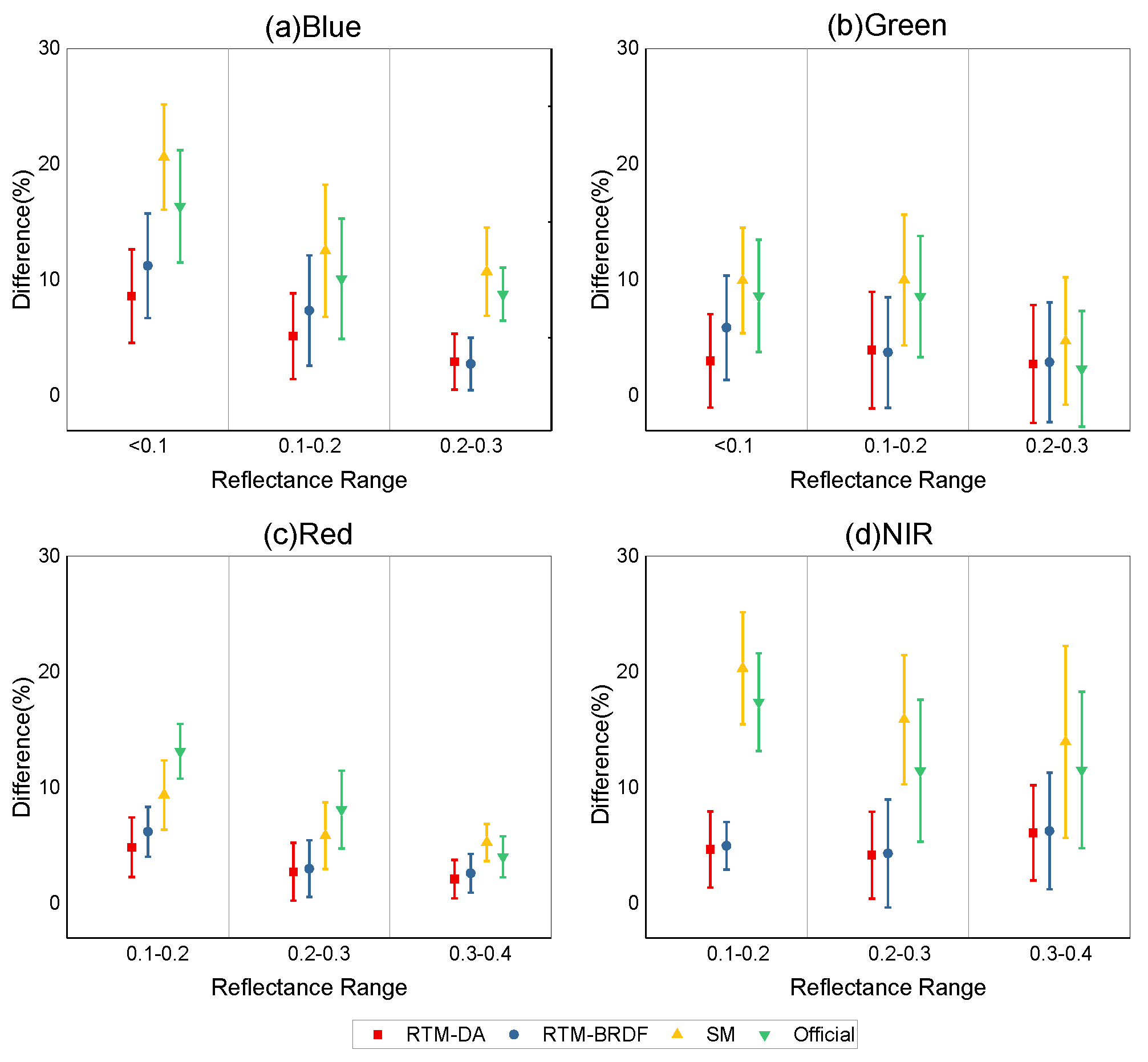
Comparisons of the surface reflectance of GF-4 PMS obtained by different calibration coefficients and the ground truths simulated by Landsat-8 OLI images are shown in Figure 8 and Figure 9. Figure 8 shows the relationships between the calibrated surface reflectance and the simulated ground truths. If the points are evenly distributed along the 1:1 line, the corresponding method obtained accurate calibration coefficients. Figure 9 plots the error bars for different reflectance ranges, determining the differences between the calibrated surface reflectance of GF-4 PMS and the ground truths.
The surface reflectance retrieved by RTM-DA agrees well with the simulated ground truth in Figure 8, as the points align the closest with the 1:1 line for the four bands compared with the other three versions of coefficients. For each band, the RMSE of RTM-DA are the smallest. The surface reflectance obtained by RTM-BRDF are also comparatively close to the ground truths, while those retrieved by SM and official coefficients are comparatively far from the true values (Figure 8). In addition, the difference between the surface reflectance derived with RTM-DA method and that simulated by Landsat-8 OLI images is the smallest for the four spectral bands, while the SM method produces the largest average differences in four bands, especially in the NIR band. For comparisons between the surface reflectance retrieved by RTM-DA and that simulated by Landsat-8 OLI image, the average difference is about 5% (Figure 8).
4.3. Uncertainty Analysis
Although the USGS spectral library was used to calculate SBAF and MODIS aerosol products were used to obtain the atmospheric parameters for atmospheric correction, there are still factors that cause uncertainties when cross-calibrating [38]. A rough estimation of potential influence that these factors have on the final cross-calibration coefficients can be described as follows:
- The uncertainty of Landsat-8 OLI calibration (σ1): The calibration uncertainty of Landsat-8 OLI for reflectance is within 3% [18].
- The uncertainty of SBAF caused by lack of ground measured spectrum (σ2): It can be seen from the Equation (8) that the calculation of SBAF requires continuous surface reflectance.
However, it is very difficult to obtain the ground measured spectrums of all the calibration ROIs. The best matched spectral curves of the calibration ROIs are found from the USGS spectral library to calculate the SBAF [39]. In order to analyze the influence of the uncertainty of the SBAF on the cross-calibration coefficients, the SBAF is increased by 0.1 and decreased by 0.1 respectively to calculate new cross-calibration coefficients, and the differences of cross-calibration coefficients before and after the change of SBAF are compared (See in Table 5). The results show that the uncertainty of calibration coefficients caused by SBAF is less than 4.5%.
- 3.
- The uncertainty caused by atmosphere parameters (σ3, σ4) [40]: In this research the parameter of the aerosol type of the 6S model was set to the desert type.
However, except for the bad weather, the aerosol type in Dunhuang area is between the desert and continental type. Thus, the aerosol type may cause error in the atmospheric correction and increase the uncertainty of the cross-calibration coefficients. To estimate the influence of aerosol type, the continental type is used as aerosol type for atmospheric correction, and then the new cross-calibration coefficients are calculated as shown in Table 6. Another atmospheric parameter visibility was calculated using the aerosol optical depth at 550 nm of the MODIS aerosol products. However, the spatial resolution of MODIS is 3km, which is quite different from that of GF-4 PM and Landsat-8 OLI. There are also significant differences in the spectra. Similarly, the visibility was changed by ±10 km to estimate the error caused by visibility to calibration coefficients. The new cross-calibration coefficients and the difference with the old cross-calibration coefficients are shown in Table 7. The results show that the total uncertainty of the cross-calibration coefficients caused by the atmospheric parameters of aerosol type and visibility is less than 5%.
Based on this analysis, the uncertainty of cross-calibration coefficients of each band () was within 7%.
5. Discussion
In this paper, a novel and simple cross-calibration based on data assimilation is proposed and implemented on GF-4 PMS using Landsat-8 OLI images. To simplify the calculation of BRDF, a BRDF adjustment factor was built to correct unequal bidirectional reflection effects. We used the data assimilation algorithm SCE-UA to optimize the BRDF adjustment factor and calibration coefficients constantly until the optimal results were found.
The calibration coefficients obtained by the proposed RTM-DA method were the closest to the officially provided version and were quite similar to those derived by RTM-BRDF method, while the SM method produced quite different results. From the validation results, we can see that the calibrated radiance and reflectance retrieved by the proposed RTM-DA method fit well with the ground truth and are quite close to those derived by RTM-BRDF method, with much smaller biases than the SM method. These indicate that for sensors with large view angles the accuracy of cross-calibration coefficients can be improved effectively after atmospheric and BRDF correction because the RTM-DA and RTM-BRDF methods take the atmosphere and BRDF effects into account while the SM method dose not. In addition, the cross-calibration and validation results of RTM-DA and RTM-BRDF were quite similar. It shows that the proposed method is a feasible and simple way to correct BRDF effect, since the RTM-DA can perform as well as the RTM-BRDF but it does not use a complex BRDF model like the RTM-BRDF. From the experiments, we can see that the proposed RTM-DA method can obtain a set of gain and offset calibration coefficients extracted from each ROI, while SM, RTM-BRDF and vicarious calibration methods can only calculate one set by fitting all ROIs. Thus, an advantage of the proposed RTM-DA method is that ROIs with large biases can be eliminated to avoid additive error to cross-calibration. Our uncertainty analysis results show that the proposed method can be used to acquire post-launch calibration coefficients of the GF-4 PMS in the future, as long as well-calibrated reference sensor data is available. Moreover, the proposed method can be easily extended to all sensors with large view angles.
6. Conclusions
Large view angles influence atmospheric radiative transfer and surface bidirectional reflectance distribution function, thus the cross-calibration of sensor data with large view angles are complex and computationally intensive. In order to solve this problem, a novel and simple method based on data assimilation is proposed and implemented to cross-calibrate GF-4 PMS using Landsat-8 OLI. An adjustment factor for the BRDF was established to correct the unequal bidirectional effects, making complex models unnecessary. The proposed method employed the Shuffled Complex Evolution-University of Arizona (SCE-UA) algorithm to find the optimal calibration coefficients and BRDF adjustment factors through an iterative process. The cross-calibration coefficients were evaluated, and the results indicated that the coefficients obtained by the proposed method were more accurate than those derived by the SM and RTM-BRDF methods, as well as the officially provided coefficients. The proposed method with low uncertainty can be used to update the calibration coefficients of GF-4 PMS in the future, and it is a feasible solution to other sensors with large view angles.
Acknowledgments
This work was supported by the National Science Foundation of China (No. 41471354) and National Key Research and Development Program of China (No. 2016YFB0502602). We would like to thank the China Center for Resources Satellite Data and Application for providing the GF-4 image data and official coefficients, and the USGS for providing Landsat-8 image data and the spectral library, the MODIS Land Team for providing the aerosol product. The reviewer’s comments are valuable which help much to improve this manuscript, and their efforts are also greatly appreciated.
Author Contributions
Yepei Chen and Kaimin Sun conceived and designed the experiments; Yepei Chen performed the experiments; Deren Li and Kaimin Sun helped to outline the manuscript structure; and Chengquan Huang helped Yepei Chen and Ting Bai to prepare the manuscript.
Conflicts of Interest
The authors declare no conflict of interest.
References
- Teillet, P.; Markham, B.; Irish, R.R. Landsat cross-calibration based on near simultaneous imaging of common ground targets. Remote Sens. Environ. 2006, 102, 264–270. [Google Scholar] [CrossRef]
- Jiang, G.M.; Li, Z.L. Cross-calibration of msg1-seviri infrared channels with terra-modis channels. Int. J. Remote Sens. 2009, 30, 753–769. [Google Scholar] [CrossRef]
- Gao, C.; Jiang, X.; Li, X.; Li, X. The cross-calibration of cbers-02b/ccd visible-near infrared channels with terra/modis channels. Int. J. Remote Sens. 2013, 34, 3688–3698. [Google Scholar] [CrossRef]
- Obata, K.; Miura, T.; Yoshioka, H.; Huete, A.R.; Vargas, M. Spectral cross-calibration of viirs enhanced vegetation index with modis: A case study using year-long global data. Remote Sens. 2016, 8, 34. [Google Scholar] [CrossRef]
- Gao, H.; Gu, X.; Yu, T.; Liu, L.; Sun, Y.; Xie, Y.; Liu, Q. Validation of the calibration coefficient of the gaofen-1 pms sensor using the landsat 8 oli. Remote Sens. 2016, 8, 132. [Google Scholar] [CrossRef]
- Gao, H.; Gu, X.; Yu, T.; Sun, Y.; Liu, Q. Cross-calibration of gf-1 pms sensor with landsat 8 oli and terra modis. IEEE Trans. Geosci. Remote Sens. 2016, 54, 4847–4854. [Google Scholar] [CrossRef]
- Mishra, N.; Haque, M.O.; Leigh, L.; Aaron, D.; Helder, D.; Markham, B. Radiometric cross calibration of landsat 8 operational land imager (oli) and landsat 7 enhanced thematic mapper plus (etm+). Remote Sens. 2014, 6, 12619–12638. [Google Scholar] [CrossRef]
- Li, J.; Feng, L.; Pang, X.; Gong, W.; Zhao, X. Radiometric cross calibration of gaofen-1 wfv cameras using landsat-8 oli images: A simple image-based method. Remote Sens. 2016, 8, 411. [Google Scholar] [CrossRef]
- Lucht, W.; Roujean, J.L. Considerations in the parametric modeling of brdf and albedo from multiangular satellite sensor observations. Remote Sens. Rev. 2000, 18, 343–379. [Google Scholar] [CrossRef]
- Li, X.; Gu, X.; Yu, T.; Li, X. Enhanced radiometric calibration coefficients for ccd camera by considering brdf of calibration sites. J. Remote Sens. Beijing 2006, 10, 636. [Google Scholar]
- Kaufman, Y.; Tanré, D.; Remer, L.A.; Vermote, E.; Chu, A.; Holben, B. Operational remote sensing of tropospheric aerosol over land from eos moderate resolution imaging spectroradiometer. J. Geophys. Res. Atmos. 1997, 102, 17051–17067. [Google Scholar] [CrossRef]
- Franch, B.; Vermote, E.; Sobrino, J.; Fédèle, E. Analysis of directional effects on atmospheric correction. Remote Sens. Environ. 2013, 128, 276–288. [Google Scholar] [CrossRef]
- Angal, A.; Xiong, X.; Wu, A.; Chander, G.; Choi, T. Multitemporal cross-calibration of the terra modis and landsat 7 etm+ reflective solar bands. IEEE Trans. Geosci. Remote Sens. 2013, 51, 1870–1882. [Google Scholar] [CrossRef]
- Feng, L.; Li, J.; Gong, W.; Zhao, X.; Chen, X.; Pang, X. Radiometric cross-calibration of gaofen-1 wfv cameras using landsat-8 oli images: A solution for large view angle associated problems. Remote Sens. Environ. 2016, 174, 56–68. [Google Scholar] [CrossRef]
- Yang, A.; Zhong, B.; Lv, W.; Wu, S.; Liu, Q. Cross-calibration of gf-1/wfv over a desert site using landsat-8/oli imagery and zy-3/tlc data. Remote Sens. 2015, 7, 10763–10787. [Google Scholar] [CrossRef]
- Yang, A.; Zhong, B.; Wu, S.; Liu, Q. Radiometric cross-calibration of gf-4 in multispectral bands. Remote Sens. 2017, 9, 232. [Google Scholar] [CrossRef]
- Chander, G.; Markham, B.L.; Helder, D.L. Summary of current radiometric calibration coefficients for landsat mss, tm, etm+, and eo-1 ali sensors. Remote Sens. Environ. 2009, 113, 893–903. [Google Scholar] [CrossRef]
- Roy, D.P.; Wulder, M.; Loveland, T.; Woodcock, C.; Allen, R.; Anderson, M.; Helder, D.; Irons, J.; Johnson, D.; Kennedy, R. Landsat-8: Science and product vision for terrestrial global change research. Remote Sens. Environ. 2014, 145, 154–172. [Google Scholar] [CrossRef]
- Hu, X.; Liu, J.; Sun, L.; Rong, Z.; Li, Y.; Zhang, Y.; Zheng, Z.; Wu, R.; Zhang, L.; Gu, X. Characterization of crcs dunhuang test site and vicarious calibration utilization for fengyun (fy) series sensors. Can. J. Remote Sens. 2010, 36, 566–582. [Google Scholar] [CrossRef]
- Chen, L.; Hu, X.; Xu, N.; Zhang, P. The application of deep convective clouds in the calibration and response monitoring of the reflective solar bands of fy-3a/mersi (medium resolution spectral imager). Remote Sens. 2013, 5, 6958–6975. [Google Scholar] [CrossRef]
- Li, J.; Chen, X.; Tian, L.; Yu, H.; Zhang, W. An evaluation of the temporal stability of hj-1 ccd data using a desert calibration site and landsat 7 etm+. Int. J. Remote Sens. 2015, 36, 3733–3750. [Google Scholar] [CrossRef]
- Wu, D.; Yin, Y.; Wang, Z.; Gu, X.; Verbrugghe, M.; Guyot, G. Radiometric characterisation of dunhuang satellite calibration test site (china). Phys. Meas. Signat. Remote Sens. 1997, 1, 151–160. [Google Scholar]
- Levy, R.C.; Remer, L.A.; Tanré, D.; Mattoo, S.; Kaufman, Y.J. Algorithm for Remote Sensing of Tropospheric Aerosol over Dark Targets from Modis: Collections 005 and 051: Revision 2; feb 2009. Available online: https://pdfs.semanticscholar.org/e5f8/fa50577584a2ef9d2ed6417b4156fb9b474b.pdf (accessed on 23 April 2017).
- Clark, R.N.; Swayze, G.A.; Wise, R.; Livo, K.E.; Hoefen, T.; Kokaly, R.F.; Sutley, S.J. Usgs Digital Spectral Library Splib06a. Available online: https://speclab.cr.usgs.gov/spectral.lib06/ds231/ (accessed on 23 April 2017).
- Thuillier, G.; Hersé, M.; Labs, D.; Foujols, T.; Peetermans, W.; Gillotay, D.; Simon, P.; Mandel, H. The solar spectral irradiance from 200 to 2400 nm as measured by the solspec spectrometer from the atlas and eureca missions. Sol. Phys. 2003, 214, 1–22. [Google Scholar] [CrossRef]
- Vermote, E.F.; Tanré, D.; Deuze, J.L.; Herman, M.; Morcette, J.-J. Second simulation of the satellite signal in the solar spectrum, 6s: An overview. IEEE Trans. Geosci. Remote Sens. 1997, 35, 675–686. [Google Scholar] [CrossRef]
- US National Bureau of Standards; Nicodemus, F.E. Geometrical Considerations and Nomenclature for Reflectance; US Department of Commerce, National Bureau of Standards: Washington, DC, USA, 1977; Volume 160.
- Roujean, J.L.; Leroy, M.; Deschamps, P.Y. A bidirectional reflectance model of the earth’s surface for the correction of remote sensing data. J. Geophys. Res. Atmos. 1992, 97, 20455–20468. [Google Scholar] [CrossRef]
- Lucht, W.; Schaaf, C.B.; Strahler, A.H. An algorithm for the retrieval of albedo from space using semiempirical brdf models. IEEE Trans. Geosci. Remote Sens. 2000, 38, 977–998. [Google Scholar] [CrossRef]
- Rahman, H.; Pinty, B.; Verstraete, M.M. Coupled surface-atmosphere reflectance (csar) model: 2. Semiempirical surface model usable with noaa advanced very high resolution radiometer data. J. Geophys. Res. Atmos. 1993, 98, 20791–20801. [Google Scholar] [CrossRef]
- Staylor, W.F.; Suttles, J.T. Reflection and emission models for deserts derived from nimbus-7 erb scanner measurements. J. Appl. Meteorol. 1986, 25, 196–202. [Google Scholar] [CrossRef]
- Roy, D.P.; Ju, J.; Lewis, P.; Schaaf, C.; Gao, F.; Hansen, M.; Lindquist, E. Multi-temporal modis–landsat data fusion for relative radiometric normalization, gap filling, and prediction of landsat data. Remote Sens. Environ. 2008, 112, 3112–3130. [Google Scholar] [CrossRef]
- Chander, G.; Mishra, N.; Helder, D.L.; Aaron, D.B.; Angal, A.; Choi, T.; Xiong, X.; Doelling, D.R. Applications of spectral band adjustment factors (sbaf) for cross-calibration. IEEE Trans. Geosci. Remote Sens. 2013, 51, 1267–1281. [Google Scholar] [CrossRef]
- Duan, Q.; Gupta, V.K.; Sorooshian, S. Shuffled complex evolution approach for effective and efficient global minimization. J. Optim. Theory Appl. 1993, 76, 501–521. [Google Scholar] [CrossRef]
- Jeon, J.-H.; Park, C.-G.; Engel, B.A. Comparison of performance between genetic algorithm and sce-ua for calibration of scs-cn surface runoff simulation. Water 2014, 6, 3433–3456. [Google Scholar] [CrossRef]
- Chen, Y.; Mei, X.; Liu, J. Geoinformatics cotton growth monitoring and yield estimation based on assimilation of remote sensing data and crop growth model. In Proceedings of the IEEE 2015 23rd International Conference on Geoinformatics, Wuhan, China, 19–21 June 2015; pp. 1–4. [Google Scholar]
- Duan, Q.; Sorooshian, S.; Gupta, V.K. Optimal use of the sce-ua global optimization method for calibrating watershed models. J. Hydrol. 1994, 158, 265–284. [Google Scholar] [CrossRef]
- Chander, G.; Helder, D.L.; Aaron, D.; Mishra, N.; Shrestha, A.K. Assessment of spectral, misregistration, and spatial uncertainties inherent in the cross-calibration study. IEEE Trans. Geosci. Remote Sens. 2013, 51, 1282–1296. [Google Scholar] [CrossRef]
- Teillet, P.; Fedosejevs, G.; Thome, K.; Barker, J.L. Impacts of spectral band difference effects on radiometric cross-calibration between satellite sensors in the solar-reflective spectral domain. Remote Sens. Environ. 2007, 110, 393–409. [Google Scholar] [CrossRef]
- Gao, H.-l.; Gu, X.; Yu, T.; Li, X.-y.; Cheng, T.-h.; Gong, H.; Li, J.-g. Radiometric calibration for hj-1a hyper-spectrum imager and uncertainty analysis. Acta Photonica Sin. 2009, 38, 2826–2833. [Google Scholar]
Figure 1.
The location of the Dunhuang calibration sites.

Figure 2.
The GF-4 PMS and Landsat-8 OLI images over the calibration sites in this study, and the red, yellow and green polygons in figure represent the ranges of gypsum, desert, and water test sites, respectively: (a) The GF-4 PMS image shows the calibration sites in Dunhuang (NIR, Red, Green); (b) The Landsat-8 OLI image shows calibration sites in Dunhuang (NIR, Red, Green).

Figure 3.
A comparison of the spectral response for the corresponding channels in the GF-4 PMS and Landsat-8 OLI.
Figure 3.
A comparison of the spectral response for the corresponding channels in the GF-4 PMS and Landsat-8 OLI.

Figure 4.
Flow chart of cross-calibration based on data assimilation.

Figure 5.
Results of spectral matching to show the mean reflectance retrieved from atmospherically corrected Landsat-8 OLI (red points) and their matched spectrum in the USGS spectral library and from field measurements (blue curves): (a) gypsum; (b) desert; (c) water.
Figure 5.
Results of spectral matching to show the mean reflectance retrieved from atmospherically corrected Landsat-8 OLI (red points) and their matched spectrum in the USGS spectral library and from field measurements (blue curves): (a) gypsum; (b) desert; (c) water.
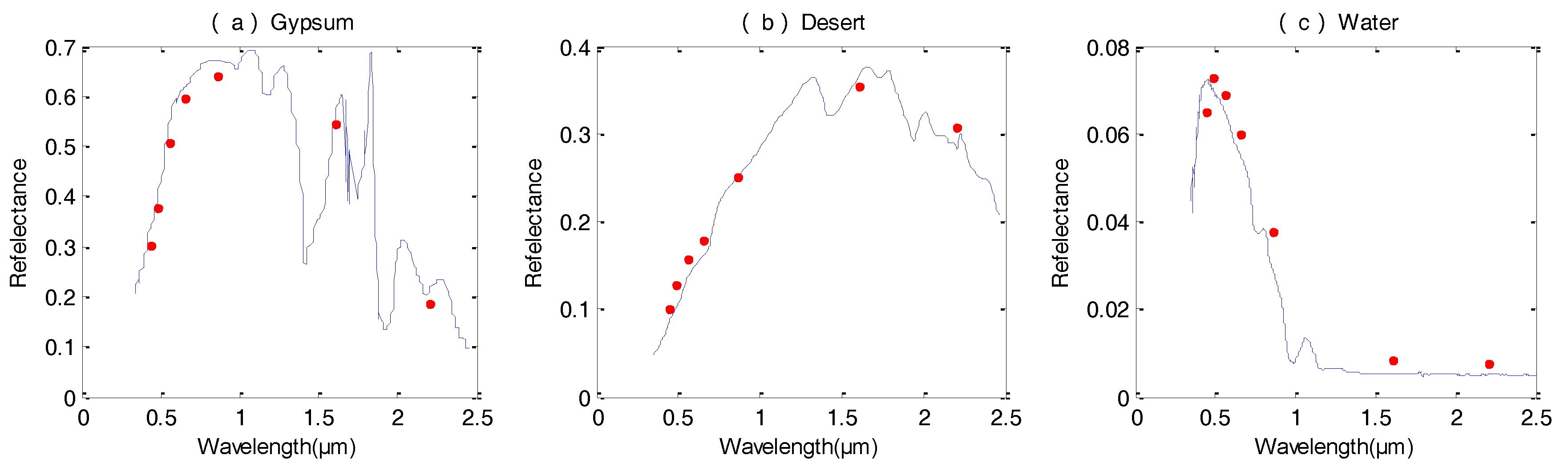
Figure 6.
Gain and offset coefficients of ROIs for the four bands of GF-4 PMS. The ROIs were sampled from water, desert, and gypsum sites, respectively.
Figure 6.
Gain and offset coefficients of ROIs for the four bands of GF-4 PMS. The ROIs were sampled from water, desert, and gypsum sites, respectively.

Figure 7.
Biases between calibrated radiance derived by the four versions of calibration coefficients and simulated radiance using Landsat-8 OLI image. The yellow points represent the radiance biases derived by the proposed method RTM-DA that have the minimum mean bias when compared with those gathered from RTM-BRDF and SM methods, as well as the officially provided coefficients.
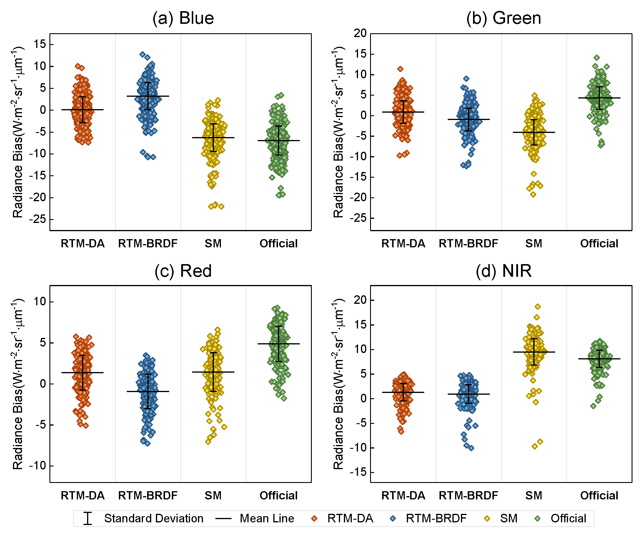
Figure 8.
Evaluation of calibrated surface reflectance of GF-4 PMS using simulated surface reflectance by Landsat-8 OLI. The results of the four versions of calibration coefficients are plotted in this figure. The yellow points represent the results derived by the proposed method RTM-DA that distribute closest to the 1:1 line for the four bands when compared to the other methods.
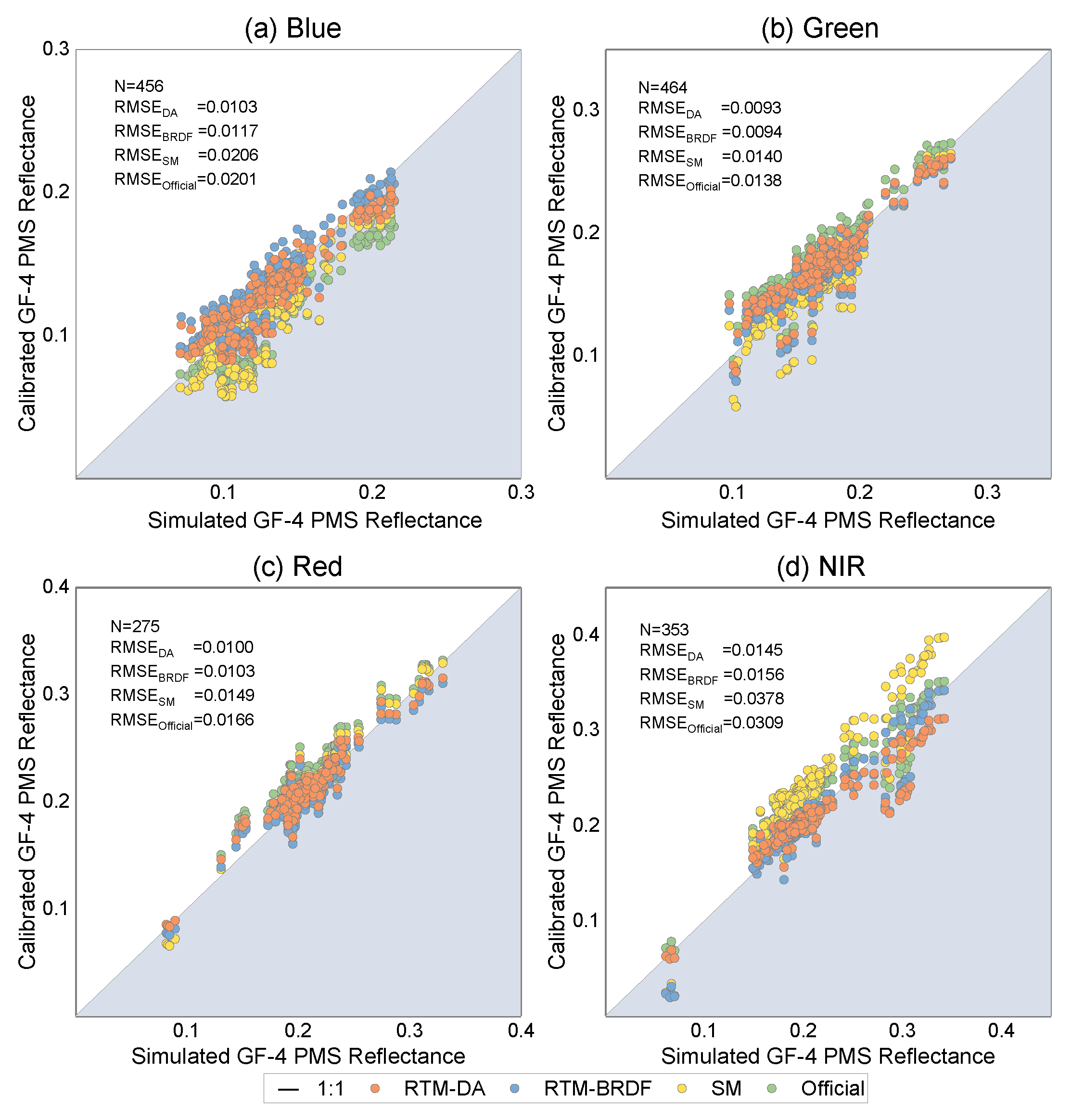
Figure 9.
The mean differences between the calibrated surface reflectance of GF-4 PMS and the simulated surface reflectance by Landsat-8 OLI. The results of the four versions of calibration coefficients are plotted. The red error bars represent the validation results of the proposed method RTM-DA with the smallest mean and variance of differences in different ranges for the four bands.

Table 1.
Comparison of the sensor parameters between Landsat-8 OLI and GF-4 PMS.
| Parameters | GF-4 PMS | Landsat-8 OLI | ||
|---|---|---|---|---|
| Band | Blue | Spectral Range (μm) | 0.44–0.53 | 0.45–0.51 |
| Solar Irradiance (W/m2/μm) | 1932.4 | 1973.1 | ||
| Center Wavelength (μm) | 0.5190 | 0.4826 | ||
| Green | Spectral Range (μm) | 0.51–0.61 | 0.53–0.59 | |
| Solar Irradiance (W/m2/μm) | 1831.6 | 1842.3 | ||
| Center Wavelength (μm) | 0.5500 | 0.5613 | ||
| Red | Spectral Range (μm) | 0.61–0.70 | 0.64–0.67 | |
| Solar Irradiance (W/m2/μm) | 1570.8 | 1564.9 | ||
| Center Wavelength (μm) | 0.6280 | 0.6546 | ||
| NIR | Spectral Range (μm) | 0.74–0.91 | 0.85–0.88 | |
| Solar Irradiance (W/m2/μm) | 1107.8 | 967.1 | ||
| Center Wavelength (μm) | 0.7700 | 0.8646 | ||
| The range of the view zenith angle | −65–70° | ±7° | ||
| Spectral Resolution (m) | 50 × 50 | 30 × 30 | ||
| Quantization (bits) | 10 | 12 | ||
| Swath (km) | 500 | 180 | ||
Table 2.
Input parameters of 6S model.
| Parameter | PMS | OLI |
|---|---|---|
| Date | 14 June 2016 | 14 June 2016 |
| Time(UTC) | 04:57:31 | 04:25:55 |
| Solar Azimuth() | 145.661 | 129.2686 |
| Solar Zenith() | 21.3436 | 23.9807 |
| Sensor Azimuth() | 161.0893 | 98.5 |
| Sensor Zenith() | 49.7657 | 0 |
| Atmosphere Model | Mid-Latitude Summer | Mid-Latitude Summer |
| Aerosol Model | Desert Model | Desert Model |
| Visibility(km) | 39.8386 | 39.8386 |
| Water Column(gm/cm2) | 1.6336 | 1.6336 |
| Ground Altitude(km) | 1.160 | 1.160 |
| Sensor Altitude(km) | 36000 | 705 |
Table 3.
Statistics of the cross-calibration coefficients of the four bands. The min, max, mean, and CV of the coefficients are listed.
Table 3.
Statistics of the cross-calibration coefficients of the four bands. The min, max, mean, and CV of the coefficients are listed.
| Band | Type | Gain | Offset | ||||||
|---|---|---|---|---|---|---|---|---|---|
| Min | Max | Mean | CV | Min | Max | Mean | CV | ||
| Blue | Gypsum | 0.1557 | 0.1977 | 0.1848 | 3.63% | −7.7429 | 8.0653 | 2.0397 | 140.08% |
| Desert | 0.1606 | 0.1988 | 0.1848 | 3.08% | −6.4067 | 9.9609 | 2.2222 | 138.75% | |
| Water | 0.1721 | 0.1983 | 0.1900 | 2.62% | −6.2856 | 8.5738 | 2.4515 | 76.14% | |
| Total | 0.1557 | 0.1988 | 0.1857 | 3.33% | −7.7429 | 9.9609 | 2.2734 | 124.85% | |
| Green | Gypsum | 0.1419 | 0.1993 | 0.1742 | 6.71% | −5.6159 | 9.7364 | 0.9451 | 157.20% |
| Desert | 0.1476 | 0.2086 | 0.1796 | 5.26% | −8.5436 | 9.4332 | 0.6668 | 130.85% | |
| Water | 0.1636 | 0.2061 | 0.1882 | 5.39% | −7.2039 | 7.9025 | 0.8945 | 179.77% | |
| Total | 0.1419 | 0.2086 | 0.1794 | 5.01% | −8.5436 | 9.7364 | 0.7127 | 138.25% | |
| Red | Gypsum | 0.1113 | 0.1604 | 0.1379 | 7.96% | −5.3937 | 6.7319 | 2.0111 | 207.35% |
| Desert | 0.1159 | 0.1765 | 0.1412 | 6.31% | −6.7027 | 9.5933 | 2.0542 | 240.70% | |
| Water | 0.1307 | 0.1582 | 0.1443 | 5.08% | −2.4281 | 7.4442 | 2.0516 | 224.50% | |
| Total | 0.1113 | 0.1765 | 0.1411 | 6.43% | −6.7027 | 9.5933 | 2.0426 | 229.24% | |
| NIR | Gypsum | 0.0820 | 0.1134 | 0.0991 | 5.68% | −6.2269 | 6.8087 | 0.8760 | 72.95% |
| Desert | 0.0714 | 0.1241 | 0.0953 | 4.04% | −9.4036 | 8.9156 | 0.7390 | 63.22% | |
| Water | 0.0646 | 0.1128 | 0.0979 | 5.60% | −6.0845 | 4.2738 | 0.7938 | 35.15% | |
| Total | 0.0646 | 0.1241 | 0.0960 | 4.15% | −9.4036 | 8.9156 | 0.7514 | 62.17% | |
Table 4.
Cross-calibration coefficients for GF-4 PMS derived from different methods as well as the officially provided coefficients. The differences between the four versions of gain coefficients are also estimated.
Table 4.
Cross-calibration coefficients for GF-4 PMS derived from different methods as well as the officially provided coefficients. The differences between the four versions of gain coefficients are also estimated.
| Band | Gain | Offset | Gain Differences (%) | ||||||||
|---|---|---|---|---|---|---|---|---|---|---|---|
| SM | RTM-BRDF | RTM-DA | Official | SM | RTM-BRDF | RTM-DA | D 1 | D 2 | D 3 | D 4 | |
| Blue | 0.2255 | 0.1988 | 0.1859 | 0.1784 | −25.5310 | −1.2218 | 2.7841 | 17.56 | 6.49 | 11.43 | 4.02 |
| Green | 0.2121 | 0.1869 | 0.1799 | 0.1878 | −22.335 | −4.6956 | 1.0837 | 15.18 | 3.75 | 0.48 | 4.21 |
| Red | 0.1604 | 0.1427 | 0.1409 | 0.1515 | −9.3643 | 0.0530 | 3.5454 | 12.16 | 1.26 | 5.81 | 7.00 |
| NIR | 0.1439 | 0.1225 | 0.0959 | 0.1080 | −21.287 | −16.323 | 0.7961 | 33.36 | 21.71 | 13.43 | 11.20 |
1 is the gain differences between RTM-DA and SM methods, 2 is the gain differences between RTM-DA and RTM-BRDF methods, 3 is the gain differences between RTM-BRDF and Official coefficients, 4 is the gain differences between RTM-DA and Official coefficients.
Table 5.
The calibration coefficients that are derived with varying SBAF and their relative difference in comparison to those depicted in Table 4.
Table 5.
The calibration coefficients that are derived with varying SBAF and their relative difference in comparison to those depicted in Table 4.
| Blue | Green | Red | NIR | ||
|---|---|---|---|---|---|
| SBAF increasing by 0.1 | New gain coefficients | 0.1867 | 0.1805 | 0.1422 | 0.0962 |
| Relative difference | 0.43% | 0.33% | 0.92% | 0.31% | |
| SBAF decreasing by 0.1 | New gain coefficients | 0.1792 | 0.1743 | 0.1351 | 0.0933 |
| Relative difference | −3.60% | −3.11% | −4.12% | −2.71% |
Table 6.
The calibration coefficients that are derived using a continental aerosols model and their relative difference in comparison to those depicted in Table 4.
Table 6.
The calibration coefficients that are derived using a continental aerosols model and their relative difference in comparison to those depicted in Table 4.
| Blue | Green | Red | NIR | |
|---|---|---|---|---|
| New gain coefficients | 0.1866 | 0.1802 | 0.1413 | 0.0964 |
| Relative difference | 0.38% | 0.17% | 0.28% | 0.52% |
Table 7.
The calibration coefficients that are derived with varying visibility and their relative difference in comparison to those depicted in Table 4.
Table 7.
The calibration coefficients that are derived with varying visibility and their relative difference in comparison to those depicted in Table 4.
| Blue | Green | Red | NIR | ||
|---|---|---|---|---|---|
| Visibility increasing by 10 km | New gain coefficients | 0.1796 | 0.1752 | 0.1365 | 0.0913 |
| Relative difference | −3.39% | −2.61% | −3.12% | −4.79% | |
| Visibility decreasing by 10 km | New gain coefficients | 0.1900 | 0.1823 | 0.1447 | 0.1004 |
| Relative difference | 2.21% | 1.33% | 2.70% | 4.69% |
© 2017 by the authors. Licensee MDPI, Basel, Switzerland. This article is an open access article distributed under the terms and conditions of the Creative Commons Attribution (CC BY) license (http://creativecommons.org/licenses/by/4.0/).
Share and Cite
MDPI and ACS Style
Chen, Y.; Sun, K.; Li, D.; Bai, T.; Huang, C. Radiometric Cross-Calibration of GF-4 PMS Sensor Based on Assimilation of Landsat-8 OLI Images. Remote Sens. 2017, 9, 811. https://doi.org/10.3390/rs9080811
AMA Style
Chen Y, Sun K, Li D, Bai T, Huang C. Radiometric Cross-Calibration of GF-4 PMS Sensor Based on Assimilation of Landsat-8 OLI Images. Remote Sensing. 2017; 9(8):811. https://doi.org/10.3390/rs9080811
Chicago/Turabian StyleChen, Yepei, Kaimin Sun, Deren Li, Ting Bai, and Chengquan Huang. 2017. "Radiometric Cross-Calibration of GF-4 PMS Sensor Based on Assimilation of Landsat-8 OLI Images" Remote Sensing 9, no. 8: 811. https://doi.org/10.3390/rs9080811
Note that from the first issue of 2016, this journal uses article numbers instead of page numbers. See further details here.