
Soil Moisture Data Assimilation in a Hydrological Model: A Case Study in Belgium Using Large-Scale Satellite Data

Royal Meteorological Institute of Belgium, Avenue Circulaire 3, B-1180 Brussels, Belgium
*
Author to whom correspondence should be addressed.
Remote Sens. 2017, 9(8), 820; https://doi.org/10.3390/rs9080820
Submission received: 16 June 2017
/
Revised: 4 August 2017
/
Accepted: 7 August 2017
/
Published: 10 August 2017
(This article belongs to the Special Issue Retrieval, Validation and Application of Satellite Soil Moisture Data)
Abstract
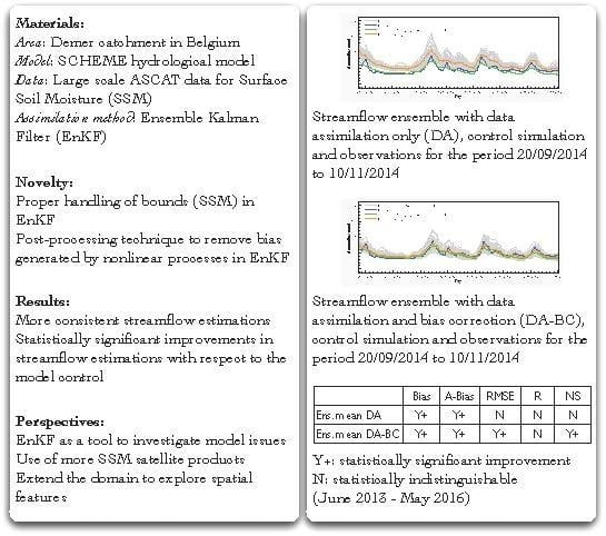
:In the present study, we focus on the assimilation of satellite observations for Surface Soil Moisture (SSM) in a hydrological model. The satellite data are produced in the framework of the EUMETSAT project H-SAF and are based on measurements with the Advanced radar Scatterometer (ASCAT), embarked on the Meteorological Operational satellites (MetOp). The product generated with these measurements has a horizontal resolution of 25 km and represents the upper few centimeters of soil. Our approach is based on the Ensemble Kalman Filter technique (EnKF), where observation and model uncertainties are taken into account, implemented in a conceptual hydrological model. The analysis is carried out in the Demer catchment of the Scheldt River Basin in Belgium, for the period from June 2013–May 2016. In this context, two methodological advances are being proposed. First, the generation of stochastic terms, necessary for the EnKF, of bounded variables like SSM is addressed with the aid of specially-designed probability distributions, so that the bounds are never exceeded. Second, bias due to the assimilation procedure itself is removed using a post-processing technique. Subsequently, the impact of SSM assimilation on the simulated streamflow is estimated using a series of statistical measures based on the ensemble average. The differences from the control simulation are then assessed using a two-dimensional bootstrap sampling on the ensemble generated by the assimilation procedure. Our analysis shows that data assimilation combined with bias correction can improve the streamflow estimations or, at a minimum, produce results statistically indistinguishable from the control run of the hydrological model.
1. Introduction
Sources of errors in model estimations are generally of two kinds, input data errors (including initialization) and model errors. One method to decrease deviations of the estimated model states from observations is to optimally “assimilate” observed data of relevant model variables into the model. Data assimilation has a long history as a modeling tool, and in the present article, we will focus on applications to hydrology, with emphasis on soil moisture and streamflow.
Soil moisture is a variable that plays an important role in a hydrological system by regulating several water exchanges and energy fluxes. There are many monitoring networks for soil moisture around the world [1,2]. The data from in situ SSM measurements are invaluable in calibrating land surface and hydrological models, while long-term time series can reveal trends due to climate or land use changes. However, in situ soil moisture measurements still remain very sparse, especially compared to the high spatial variability of this variable.
Satellite observations can ensure today complete coverage of large areas and provide a representation of the soil state at regular time intervals. Specifically, as an alternative to ground-based measurements, great efforts have been made in the past two decades to develop soil moisture products from microwave signals with the launch of several instruments on board satellite missions [3,4,5,6,7,8]. Examples of such satellite sensors are the Special Sensor Microwave Imager (SSM/I) on board a series of Defense Meteorological Satellite Program platforms, the Tropical Rainfall Measuring Mission (TRMM) Microwave Imager (TMI) by NASA, the Advanced Microwave Scanning Radiometer-Earth Observing System (AMSR-E) by NASA, its successor AMSR2, the Soil Moisture and Ocean Salinity (SMOS) by ESA, the Soil Moisture Active Passive (SMAP) by NASA and the ASCAT sensor by EUMETSAT. In particular, in [8], a Land Parameter Retrieval Model (LPRM) is used for surface soil moisture retrievals in order to generate long global series of data. A special algorithm for hydrological applications (HydroAlgo) has been developed in [9] and used to generate maps of snow depth and soil moisture content from AMSR-E and AMSR2 data.
Each satellite mission carrying such instruments has been designed to satisfy certain technical requirements, e.g., regarding spatial coverage, resolution and scanning frequency. Therefore, significant differences can be expected between the technical specifications of satellite data and the corresponding requirements of several applications in Earth systems, e.g., modeling of the atmosphere and of the hydrological cycle. In fact, many studies have investigated the potential to improve river discharge estimations by using satellite data in hydrological models. This is a complex task, and the outcome depends on the model used, the spatiotemporal scales, the method of using the data (direct use or assimilation) and the quality and availability of the satellite data. For example, [10] obtain improvements in flood forecasting by complementing discharge data assimilation with soil moisture data assimilation.
Several other studies exist investigating potential benefits of assimilating soil moisture data, e.g., [11,12,13,14,15], with encouraging or mixed results. In particular, in [13], the authors conclude that the underestimation of the vertical soil coupling in the SWAT model impedes the ability of data assimilation to update deep soil moisture. On the other hand, in [16], soil moisture products have been successfully used in a simplified continuous rainfall-runoff model in order to provide initial wetness conditions prior to a flood event, demonstrating that these products contain useful information, which can be exploited in flood forecasting. Such studies highlight the issues that may arise due to model structure, catchment characteristics and observation errors.
Another frequently-encountered problem is the difference, or bias, in the mean value and variability between different sources of SSM data (satellite retrievals and model integrations in our context). This bias can pose significant obstacles to the use of the information contained in satellite measurements for any kind of application, including data assimilation, and has to be removed. Different methods to remove such bias have been explored in the literature, in particular linear regression, mean and variance matching and Cumulative Distribution Function (CDF) matching [14,17,18,19,20,21]. In [21], the authors show that proper pre-processing of soil moisture observations can be critical for the performance of the data assimilation.
Estimating an appropriate error for soil moisture observations, used in data assimilation, is still an open problem. One choice is to compare the satellite data with ground-based observations (validation) [22]. Independent estimations of the error are also possible, e.g., based on triple collocation [23] and Fourier transforms [24]. The main difficulties are the higher uncertainty and coarser spatial resolution of the satellite observations, compared to ground-based measurements, and the errors associated with the retrieval algorithms. For an extensive discussion of such issues arising in SSM data assimilation into a hydrological model, we refer the reader to [25] and the references therein.
The ensemble Kalman filter is a data assimilation method used in geosciences [26,27] and in hydrology in particular [28]. It is a generalization of the common Kalman filter [29], appropriate for non-linear systems without the need to calculate the adjoint model. However, it was eventually acknowledged that the use of the stochastic terms required by this method may lead to biased estimations if the model includes non-linear processes [28,30]. This problem has been considered in other studies too, and a solution has been proposed in [11,31]. This solution can be used in cases where the assimilated variable is unconstrained, which is not the case for soil moisture. This is why the approach of [31] required repeated application of the method in order to further reduce the residual bias due to the bounds of soil moisture. A different problem, but still related to bias, is tackled in [32], where the EnKF is used in order to find an optimal method to reduce model biases.
The existence of bounds for the assimilated variable gives rise to another problem as well. In the ensemble Kalman filter, the generation and use (as perturbations) of stochastic terms from a normal distribution are generally required. Obviously, repeated application of such perturbations on a bounded variable, like soil moisture, will often drive out of their bounds the values that are already near them. This is another source of biases in the estimations, especially in the most extreme cases (very dry or very wet conditions, speaking of soil moisture). A technique based on variable standard deviation was introduced in [33] to solve this problem. Although this method reduces the bias due to exceedance of the bounds, it does not completely eliminate it.
In the present study, our goal is to assimilate satellite data for surface soil moisture in the SCHEME hydrological model and to assess the effects of this assimilation in terms of streamflow. The satellite data for soil moisture that we use here are derived from active microwave measurements with the ASCAT sensor on board the MetOp [7]. The derivation of soil moisture values from such measurements relies on a change detection method [34]. ASCAT data have been already validated using in situ measurements in southwestern France [35] yielding encouraging results; see also [36,37]. More extensive validation of such data makes up part of the ongoing EUMETSAT project H-SAF. We focus here on the case of a catchment in Belgium while our methodology aims to address the two problems in EnKF pointed out previously.
In our approach, surface soil moisture is properly treated as a bounded variable. In particular, the perturbations needed for the ensemble Kalman filter are generated from truncated normal distributions. This ensures that no soil moisture value exceeds the bounds after the application of perturbations. We use truncated distributions in order to generate perturbations for the precipitation, as well, which is thought of as the forcing of the hydrological model. In this case, the perturbations are applied multiplicatively; therefore, truncated log-normal distributions are used. Of course, precipitation is not bounded in theory from the top, and simple log-normal sampling would suffice. The reason for this unusual, at first sight, choice is that it will ensure that the precipitation values that will be generated by applying such perturbations will remain within the climatological margins.
We tackle in the following way the issue of bias, induced by non-linear processes in conjunction with the use of stochastic terms. Initially, a full data assimilation run is performed. Then, another run is performed in which only perturbations are applied to precipitation, that is the model states are not updated by the Kalman equation. The streamflow ensemble generated by this run is carrying only the bias of the process because there is no assimilated information. The deviation of its mean from the control simulation for the streamflow is then used in order to remove the bias from the full data assimilation ensemble. The introduction and use of truncated probability distributions in a data assimilation scheme and the post-processing technique explained above are the two main advances proposed here.
The article is organized as follows. In Section 2, we present a description of the hydrological model and the technical details of the assimilation methodology, including the handling of bounded variables and of bias under the presence of non-linear processes. Subsequently, in Section 3, we deal with the study area and the data used in the numerical experiments. The results are the subject of Section 4. We conclude by providing more insight in Section 5.
2. Methods
2.1. Model Description
The SCHEME hydrological model (SCHEldt-MEuse, from the names of the two major rivers of Belgium), used for our simulations, is the distributed version of the IRMB hydrological model [38]. The IRMB model has been successfully applied to various catchments ranging from about 100–1600 , representing several hydrologic conditions in Belgium (e.g., [39]). It has been used to study the climate change impacts on the water cycle under given scenarios in Belgium and Switzerland [40,41,42].
The SCHEME model is optimized for river basins up to 20,000 . The hydrological processes are lumped within grid cells of 49 , allowing one to describe the heterogeneity of hydrologic conditions and of hydrometeorological input data. With this design, the SCHEME model is able to simulate a variety of basins and hydrological conditions in the river Scheldt and Meuse River Basins in Belgium and upstream in France. It is currently being used in medium-range streamflow forecasts [43,44].
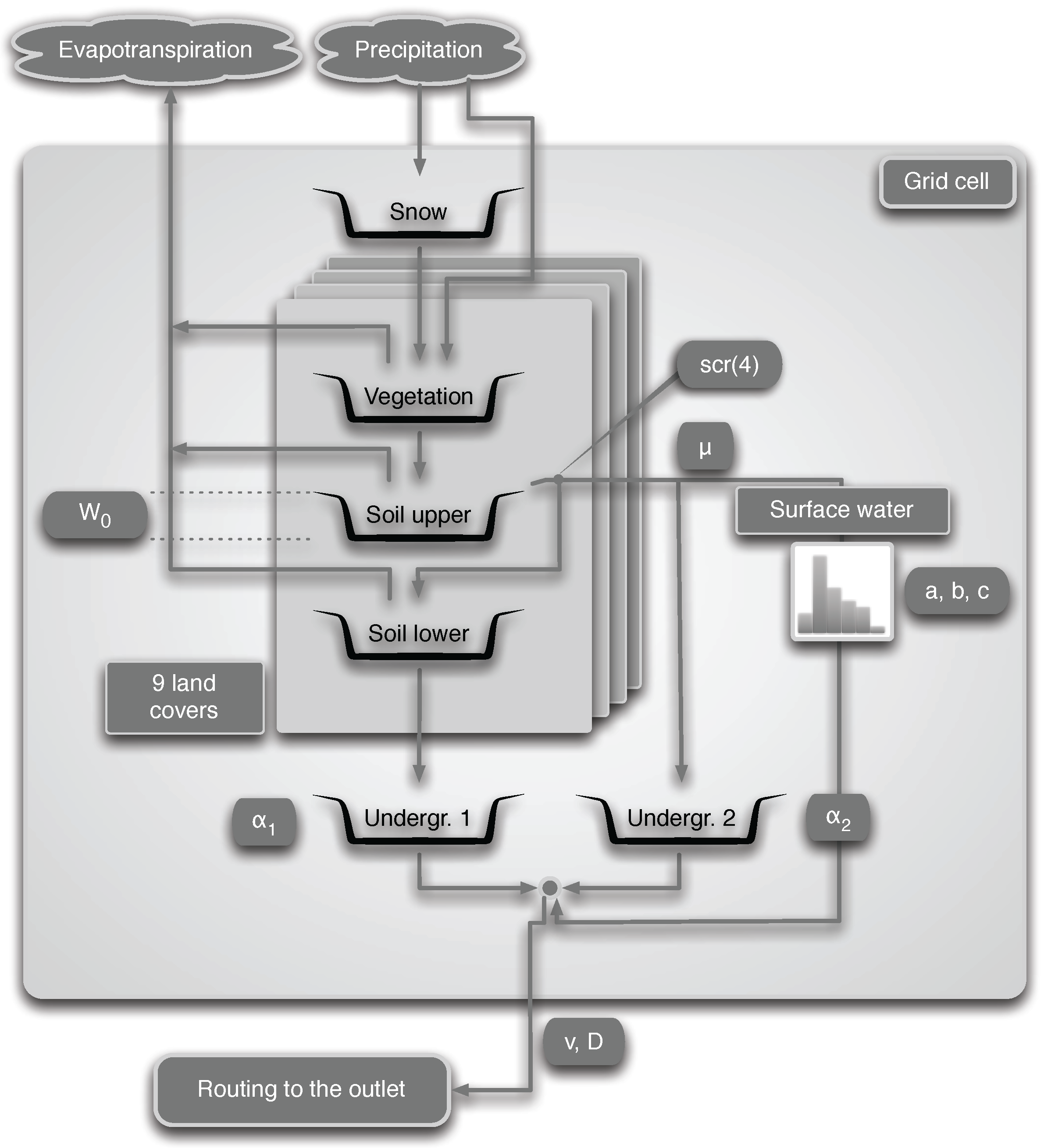
The SCHEME model structure comprises 9 different land covers with a snow accumulation and melting module. The land cover types are represented by the appropriate variable fractions on each grid cell. Sub-grid soil properties are also indirectly taken into account through a regionalization procedure. The actual evapotranspiration is calculated on the basis of the water intercepted by the vegetation and the water content of two soil layers, as well as the Potential Evapotranspiration (PET) according to the Penman formula. The time step of the model is equal to one day. Surface water is simulated with a unit hydrograph, and the underground water is represented with two reservoirs. The streamflow produced on each grid cell is routed to the outlet with a 1D submodel based on the width function of the river network [45]. A sketch of the SCHEME model mechanisms is presented in Figure 1.
Let us recall briefly from [38] the soil water balance mechanism in the SCHEME model. The general principle is the same for the two soil layers. Let and be the water contents of a given soil layer at the beginning and the end of day j, respectively, the water content when the soil is saturated and the difference between recharge and potential evapotranspiration in day j for the same soil layer. For the upper layer, the recharge is the absorption prior to all surface flooding, and for the lower layer, the recharge is the quantity of the water that infiltrates during the flooding phase. If the capacity of the lower layer is exceeded, then the excess water is percolated to one underground reservoir of the model. If , then the water content of the soil will be decreased according to the following equation:
If instead , then the water content will be increased as:
Overall, in the SCHEME model, the soil water content and runoff calculation is based on simple water balance considerations. In other studies, while analogous principles are used for soil moisture, the runoff is estimated using the Soil Conservation Service Curve Number [12,13,14]. The PDM model [11,46] is more like the SCHEME model in the sense that runoff production is controlled by the storage capacity of the soil in the context of a conceptual approach. However, an important difference is that in the PDM model, the storage capacity is treated as a random variate to account for spatial variability. A different approach is adopted in the TOPMODEL, where the spatial patterns of soil moisture are regulated by shallow groundwater gradients [15]. It is assumed that these gradients can be estimated from local topography. Runoff generation in the TOPMODEL is based on saturation and infiltration excess mechanisms.
The parameters of the SCHEME model have been calibrated based on data from a variety of catchments in the Scheldt and the Meuse River Basins from the period 1981–1988. The calibration technique combines elements from the approach in [38] and an automatic algorithm, the “Shuffled Complex Evolution of the University of Arizona” (SCE-UA; [47,48]), which has been proven efficient in locating globally-optimal parameters of hydrological models. The objective function to optimize in this case is the daily root mean square error. After calibration, the parameters are regionalized over the corresponding basins with the use of Artificial Neural Networks (ANN, NevProp software, Version 3, [49]) and geographic indices. These indices are derived from the CORINE Land-Cover (http://www.eea.europa.eu/publications/COR0-landcover) and the Soil Map of the European Countries at 1:1,000,000 [50]. First, empirical relationships are being sought between parameter values (the predictands) and indices (the predictors) over the set of catchments used in the calibration step. For each parameter, several indices are combined, an ANN model is trained and the correlation between the predicted values by the ANN model and the predictands is calculated. The correlation is corrected for overfitting with a bootstrap sampling [51] among the catchments in the following way. A model based on the same predictors is trained on the bootstrap sample. The correlation between the values predicted with this model and the predictands is calculated on the bootstrap sample. Then, the same model is applied on the full sample (including all catchments), and a new correlation is obtained. This process is repeated, and the average of the difference between the two correlation values provides an estimation of the bias to remove from the correlation obtained with the full model on the full sample. Different models (combinations of indices) are tested, and the selection is based on the unbiased correlation. Then, the model is applied over the whole basin, including areas not covered with the catchments used for calibration. The sample of parameter values provided by the bootstrap procedure is also used to estimate the model error term in Equation (5), as will be explained in Section 3.
The capacity of the upper soil layer is one of the parameters of the model that are optimized and regionalized. Its value is in the range of 5–28 mm in the Scheldt River Basin and corresponds to a soil depth of several centimeters. The saturation of this conceptual reservoir is put into correspondence with the soil wetness index of the satellite product.
2.2. Assimilation Methodology
2.2.1. General Context
Our data assimilation approach is based on the ensemble Kalman filter technique [26]. The EnKF is derived from the standard Kalman filter [29] by generating ensembles to account for model and forcing uncertainties in the presence of nonlinear processes. The goal is to optimally merge model predictions with observations, by providing estimations of the error covariance matrix based on the ensemble of the model states generated with this technique. This procedure effectively eliminates the need to linearize the model used in the simulations.
The general principles of the EnKF can be described as follows. We restrict our interest in finite dimensional systems described by ordinary differential equations. If S is the (differentiable) phase space of such a system and a trajectory of the system in it, subject to the dynamics defined by the vector field F, then we have:
In discrete form, Equation (3) reads:
where k denotes the time step, the system state at time step k and the function (set of algebraic operations) that must be applied on in order to calculate , arising from the discretization of the initial dynamical system. In our context, arises from a model, and we can write:
where the term represents the errors and the uncertainties in the model.
Let z represent the measurements of the physical quantity related to the model variable y. If the true model state is denoted by m, then we introduce the measurement operator H by the following equation:
where represents the measurement error. In practice, it is often assumed that is normally distributed. We extend the discretization notation of Equation (4) to the other variables as well. Thus, we will write .
During assimilation, the model states are adjusted using information from the observations of the variable z. In order to avoid confusion, we denote the variable y, as calculated by the model without any update, by (a-priori or forecast) and the same variable updated through assimilation by (a posteriori or analysis). Let finally denote the ensemble members, . For example, we would write for the i-th a priori ensemble member at time step k, and therefore, .
Under these conventions, the updated state at time step k is given by the equation:
where is the so-called Kalman gain matrix at time step k, given by:
In Equation (8), is the error covariance matrix for the forecast estimate obtained from the ensemble [26] and R is the variance of the noise term . As customarily, the exponent T denotes the transpose of the underlying matrix.
In our case, there is only one variable to assimilate, SSM from satellite observations. Therefore, the assimilation problem is one-dimensional, and all of the matrices involved are simply real numbers. We will consider as true model state m the satellite observation z corrected for bias using as a reference the SSM state calculated by the SCHEME model. In this setting, the measurement operator is simply the ratio , with , being the bias function when we express the SSM as a percentage. Details will be provided in subsequent sections of this article.
2.2.2. Bounded Variables
One particular feature of soil moisture is that it is bounded between the values 0 and 100. Therefore, during assimilation in an EnKF context, applying Gaussian noise on SSM will often violate this constraint, especially for values near the bounds. This is a long-standing problem that was, to our knowledge, not adequately addressed so far. A method using the variable standard deviation for the error distribution is proposed in [33]. This solves the problem partially because it reduces the frequency of the bound crossing, but it does not completely eliminate it. Furthermore, the choice of very small standard deviations for variable values near the bounds may not be always the most appropriate. Our solution is based on the concept of the truncated probability distribution [52]. This is a conditional distribution resulting from the restriction of the domain of a given probability distribution. Formally, let X be a real random variable with probability density function f and cumulative distribution function F. Then, the restriction of X on the interval is described by the distribution defined by:
where:
We notice here that , or simply when the interval is well understood, is essentially a rescaling of f over the given interval so that its integral on it (the probability) is equal to 1. Based on Equations (9) and (10), one can derive all of the properties of a truncated distribution necessary for the calculations. For the needs of the present article, we implement sampling algorithms for two distributions of this kind, truncated normal and truncated log-normal.
A truncated variable will be used in our context in the following way. Let us consider an SSM value, for example . We want to add to a noise term , coming from a normal truncated distribution with mean value 0 and standard deviation . Since the sum has to be between 0 and 100, we have . This defines the range in which has to be restricted.
We need such additive truncated variables in order to generate the variance R of the noise term (Equations (6) and (8)) and to model uncertainty regarding SSM calculations by the SCHEME model (term in Equation (5)). For the case of the variance R, we use a truncated normal distribution with . This value is in the range obtained from the validation of SSM satellite data (ERS and ASCAT) in Northern France (Grand Morin), using in situ soil moisture measurements [53].
We work similarly with truncated log-normal distributions, which are used to generate multiplicative factors. These factors constitute an implementation of the uncertainty in interpolated precipitation, which is one of the input fields in the SCHEME model. In existing literature, this uncertainty is represented as a rule by full range log-normal distributions [12]. However, in our case, allowing the full range log-normal terms can generate completely unrealistic amounts at certain rainfall events, very far away from the limits in which the SCHEME model has been calibrated and known to perform well. Using truncated log-normal distributions instead, conditioned by the climatology of the Demer catchment, solves this problem.
2.2.3. Non-Linear Processes
The ensemble Kalman filter can be used, by its design, in non-linear systems without the need for developing a linearization scheme, like for example in the case of the extended Kalman filter. This has the potential to considerably simplify the study. On the other hand, it became at some point clear that the stochastic terms generated by the filter generally induce bias in the estimations when non-linear processes take place [30].
It is possible to implement a correction method for this bias in order to make evident the net effect of the assimilation procedure. Such a method has been proposed in [31]. The case of the SCHEME model considered here is however more special, and we deal with biases in a different way.
In the SCHEME model, the calculation of moisture at the top layer of the soil is carried out as follows. Let be the physical surface soil moisture and W the model variable that represents this moisture. The value of W at each time step depends on throughfall and residual potential evapotranspiration. If it is less than or equal to the capacity of the upper soil layer (Figure 1), then it provides directly the physical soil moisture for the given time step: . However, the SCHEME model allows W to exceed , according to precipitation, which determines throughfall and evaporation conditions. When this happens, W can be written as: , where the term S is used by the model to calculate contributions to the streamflow and to the lower soil layer. In this case, the physical soil moisture of the upper soil layer coincides with the capacity: .
This simple condition on the range of W is at the origin of the non-linear behavior of the SCHEME model in the calculation of SSM. In order to quantify the effect of the stochastic terms used by the ensemble Kalman filter, we generate two different ensembles for the streamflow. Let be the streamflow ensemble generated by running as usual the full assimilation procedure and , , be the streamflow ensemble generated by running the model while keeping active only the precipitation perturbations. This means in particular that the state updates through the Kalman equation are switched off. Therefore, the members of do not carry information from satellite data. Let also be the control simulation of the model. If is the average of the ensemble at each time step k, then the daily value of bias is given by and the corrected streamflow ensemble by:
The notation convention is the same for all of the ensembles , and . Another option here is to express the bias as a ratio in order to avoid possible negative values (e.g., in models with large biases). However, the results presented here are obtained with Equation (11), since in our case, this correction yields well-defined (nonzero positive) streamflow values. Trying the ratio version of the bias produces slightly different statistical scores in Table 1, Table 2, Table 3 and Table 4 and exactly the same statistical significance results in Table 5, Table 6, Table 7 and Table 8 (Section 4).
The reason to examine the effect of precipitation perturbations only is that among the three transformations that affect directly the soil moisture variable W, namely the precipitation and soil moisture perturbations and the Kalman equation, only the first one has the potential to drive W out of range and therefore to activate the decomposition . The other two preserve the bounds: the soil moisture perturbations by construction (truncated normal distribution sampling); and the Kalman equation because it is a convex linear combination of two variables in the same interval. In other words, the precipitation perturbations are at the root of the non-linear effects in this case.
The bias correction method proposed in this section presents some analogies with the method of [31] as applied in [11]. However, the two are fundamentally different. In our approach, the forcing perturbations are applied while the data assimilation is disabled. This generates a new ensemble carrying only the effects of the non-linear processes. The new ensemble is then used in order to remove the bias due to non-linearity. In [11], the data assimilation is applied, but without the forcing perturbations. This results in a unique time series (unperturbed model prediction) used as the baseline to remove the bias. According to our knowledge, the bias correction method proposed here is new and has not been used in previous studies.
3. Study Area and Data
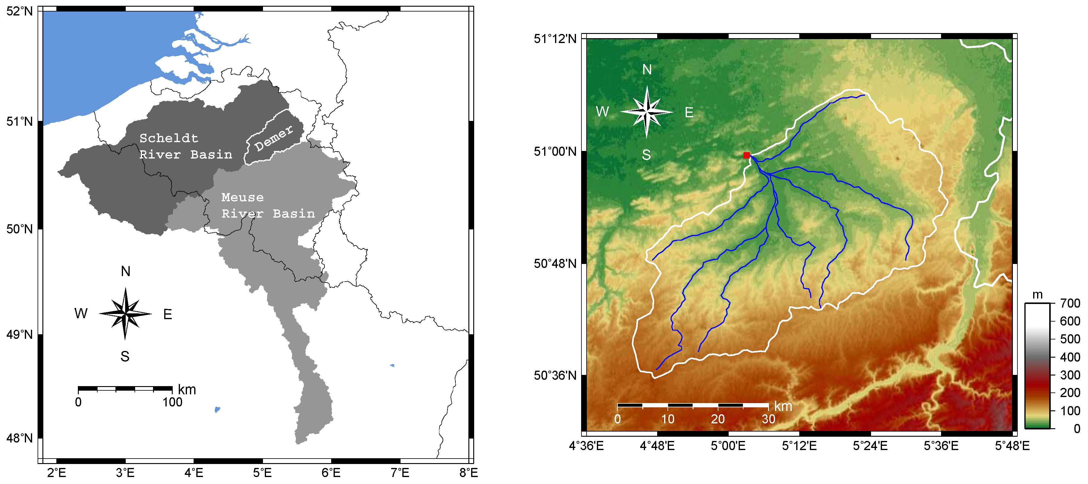
Our study is carried out for the catchment of Demer, located in the central-eastern part of Belgium. This catchment covers an area of and makes part of the Scheldt River Basin (see Figure 2).
The main land use in the Demer catchment consists of crops (46%), meadows (29%) and forests (18%). The remaining 7% is inhabited. The elevation ranges between 17 and 173 meters, with a mildly hilly profile in the south. The length of the main river is . For the period 1971–2000, the average runoff is about s () and the coldest ones are January s () and daily minimum of s ().
A rain gauge network from the Royal Meteorological Institute of Belgium (approximately one station per ) provides daily rainfall data in the Demer basin. For the period 1966–1995, the average yearly precipitation in the catchment is about . The rainiest month is June, with of rainfall, and the driest one is April with . Therefore, the precipitation is quite uniformly distributed throughout the year, typical for an oceanic climate under some continental influence. The spatial distribution of precipitation is also quite homogeneous due to the almost flat topography of the area.
In the same reference period (1966–1995), the mean temperature is in the Demer catchment. The hottest months are July and August, with and , and the coldest ones are January and February with and respectively.
The study period is 1 June 2013–31 May 2016. The satellite data we use for this period come from the EUMETSAT Satellite Application Facility on Support to Operational Hydrology and Water Management (project H-SAF, http://hsaf.meteoam.it/). However, older data starting in June 2009 have been used in order to calculate bias correction for soil moisture.
For assimilation purposes, we use the large-scale surface soil moisture product SM-OBS-1(or H07). This product is generated from MetOp scatterometer data (ASCAT) at a coarse resolution () controlled by the IFOV of the instrument and provides data for the surface layer of the soil (0.5–2 cm). The measurement of soil moisture with the MetOp scatterometer is fairly direct because of the high sensitivity of the microwaves to the water content of the upper soil layer. This is carried out using the so-called TU-Wien change detection method [54]. However, the different contributions to the observed total backscatter from the soil, vegetation and soil-vegetation interaction effects cannot be separated. The main assumptions in this approach are linearity in the relation between the backscattering coefficient and surface soil moisture content, stability in time of roughness and land cover and the influence of the vegetation phenology on backscatter at the seasonal time scale only. Snow and frozen soil conditions are not treated in the change detection method, and special care should be taken, using auxiliary information, in order to avoid spurious contributions in winter. In the Demer catchment, forests and topography have a rather limited influence (see Figure 2 and the catchment metrics in the beginning of this section). Snow presence is also quite limited. The main concern is freezing conditions. We address such issues in the present study by deactivating data assimilation when the mean air temperature falls below 2.0.
We also use the H-SAF product SM-DAS-2 (or H14) for comparisons with the SCHEME model data at the root zone level. This product is generated in the ECMWF Land Data Assimilation System by assimilating ASCAT SSM data (essentially the H07 product that we discussed previously). In this case, the data assimilation process is based on the extended Kalman filter [55]. The ECMWF model generates soil moisture profiles according to the Hydrology Tiled ECMWF Scheme for Surface Exchanges over Land (HTESSEL, [56]) providing estimations for four soil layers for a total thickness of below the surface. SM-DAS-2 is available at a spatial resolution of with a daily time step.
Before assimilating the SSM data from H07, a bias correction is applied on them in order to determine the true state in Equation (6). The H07 data used for this purpose cover the period from June 2009–May 2013, and the reference data are obtained from the output of the SCHEME model. First, the spatial averages over the Demer catchment of all of the necessary data are calculated to produce two four-year-long times series, one from H07 and another one from the model. The bias correction is based on the difference between the distributions represented by the two time series (CDF matching, [19]). In Figure 3, we can see the bias as a function of the soil moisture value. Obviously, a piecewise linear interpolation can be used in order to obtain a bias function defined everywhere.
As mentioned in Section 2, the satellite data are treated in EnKF as random variables (Equation (6)). This is also useful in the implementation of the data assimilation procedure. In particular, during data assimilation, each pixel of the SCHEME model grid is matched with the closest satellite pixel. This means that about ten SCHEME model pixels are matched with the same satellite pixel. However, the corresponding satellite value is perturbed independently for each model pixel and natural cover inside that pixel, using truncated normal distributions as explained in Section 2.2.2. This approach yields different perturbed satellite values for each time step, pixel and sub-pixel features of the SCHEME model.
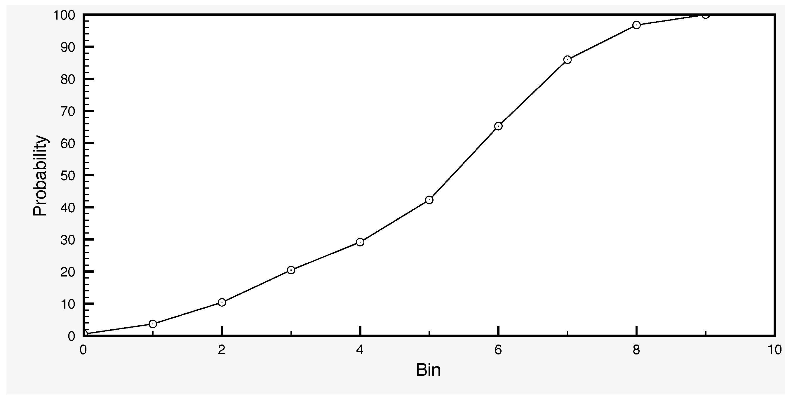
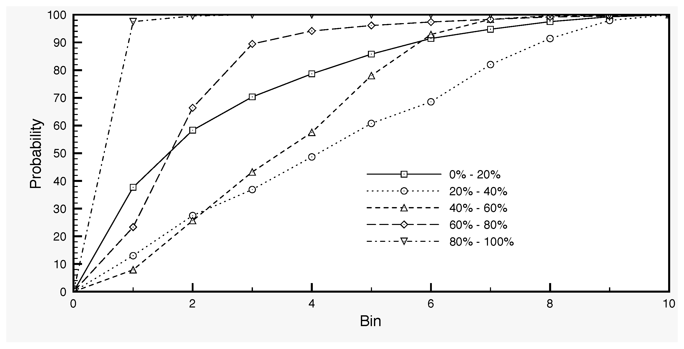
The model error term in Equation (5) is calculated as follows in our case. By varying a set of parameters of the SCHEME model, we generate an ensemble of SSM time series with 100 members, as the output of the model runs. Each parameter set defines a variant of the model, which is used in order to produce a long time series of 30 years (1966–1995) for surface soil moisture. In this way, we generate the ensemble of SSM model output. We work with this dataset by dividing first the full SSM range into five classes: 0–20%, 20–40%, 40–60%, 60–80% and 80–100%. These data are then used in order to determine the distribution of the SSM values (Figure 4) and, for each SSM class, the distribution of the standard deviations (Figure 5). The former is used in the generation of the initial SSM ensemble at the start day of the assimilation, while the latter in the generation of the error (Equation (5)) by sampling a truncated normal distribution.
For the generation of the term of a given SSM value, we first draw a value from the uniform probability distribution on the interval [0,1]. Using the data represented in Figure 5, we can then determine the corresponding bin. This bin makes part of the subdivision of the standard deviation interval, which is known and corresponds to the class to which the given SSM value belongs. With this information, we can determine the (randomly drawn) standard deviation corresponding to the given SSM value. Subsequently we use in order to define the truncated normal distribution and randomly draw from it the term , as described in Section 2.2.1. The probabilistic context for the generation of the standard deviation and, subsequently, of the term described above is new and has not been used in other studies according to our knowledge.
In an analogous way, the perturbations for precipitation (Section 2.2.2) are generated by sampling a truncated log-normal distribution with the mean equal to one and the standard deviation that depends on the precipitation value. The dependence is determined empirically based on the climatology of the Demer catchment and the ensemble verification measures for streamflow, described in [30]. In this way, the perturbed precipitation is lying always within the interval in . This interval covers all of the cases of daily rainfall in the calibration period of the SCHEME model. The truncated perturbation approach in this context guarantees that no unrealistic precipitation events will be generated during the execution of the data assimilation procedure. Exaggerated precipitation can become a problem with the use of unbounded probability distributions (see Section 2.2.2), and it has not been previously addressed in the existing literature. The same principle holds for any model sensitive to certain forcing variables.
4. Simulations and Results
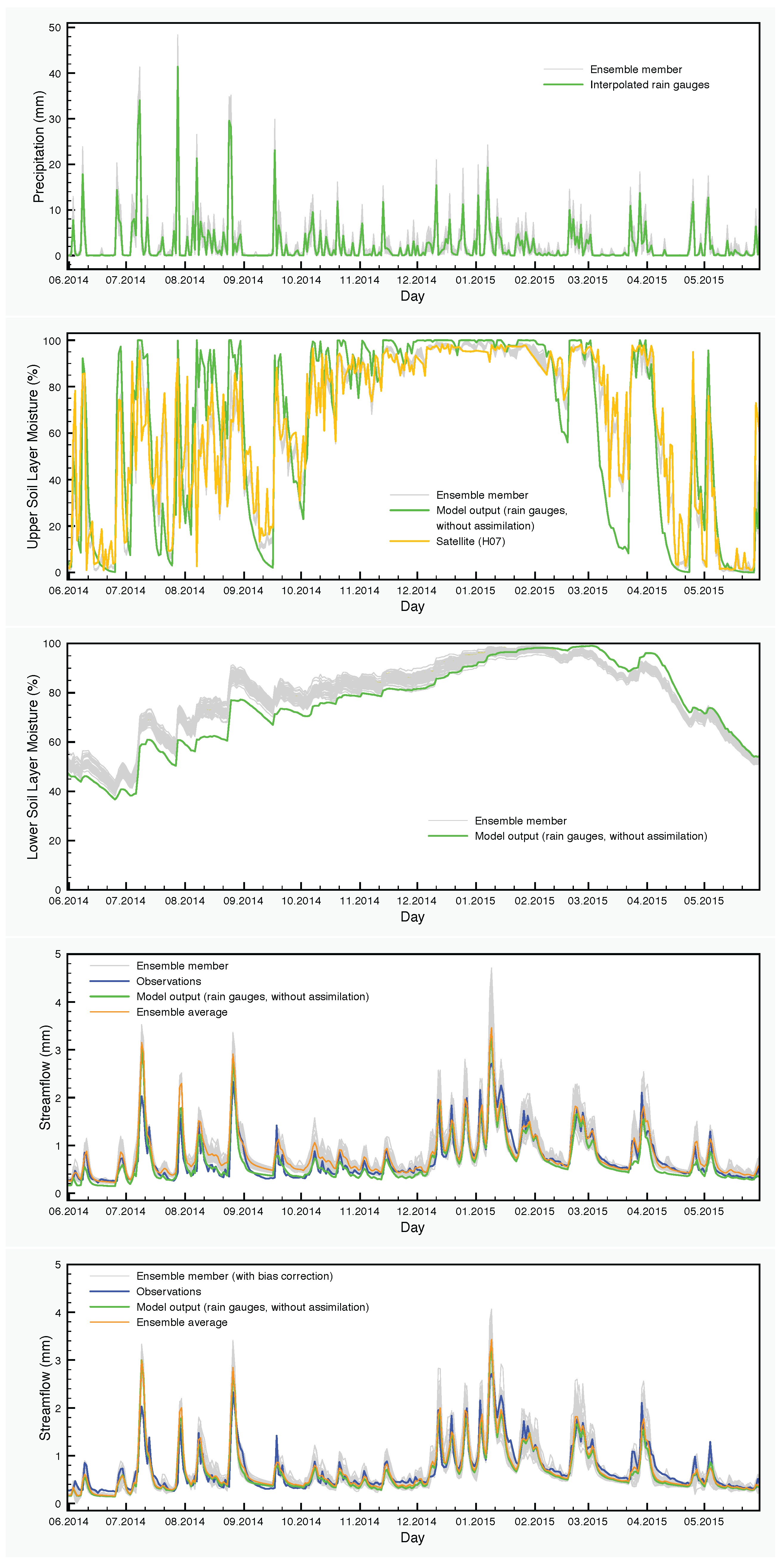
The precipitation input and the results of simulations with the SCHEME model are graphically represented in Figure 6, Figure 7 and Figure 8. Each figure corresponds to one of the three years of the study period (June 2013–May 2016). The precipitation and the soil moisture in the two layers of the model are reduced to time series by calculating the areal averages of the corresponding fields over the Demer catchment.
The effect of the assimilation is very obvious at the level of the soil moisture. Regarding the upper layer of the soil, the ensemble generally follows the satellite values. The situation is very different in the lower soil layer, where no assimilation is taking place, but the moisture values are calculated by the SCHEME model after assimilating satellite data at the upper layer. The results of the reference simulation are the only basis for quantitative comparisons that we have for this layer of the soil. In some cases, we observe large deviations between the ensemble members and the reference simulation (e.g., autumn and winter in Figure 8).
For the streamflow, we have two cases, one ensemble obtained by applying the assimilation procedure (DA) and another one obtained by correcting the previous ensemble for bias (DA-BC), according to the method described in Section 2.2.3.
In the corresponding figures, the ensemble averages are also depicted together with the control simulation of the model and the streamflow observations. The differences between these time series are quantified using well-established synoptic statistical measures such as bias, Absolute bias (A-bias), root mean square error (RMSE), correlation (R) and Nash–Sutcliffe Efficiency coefficient (NSE). The calculations are carried out at seasonal and annual time scales. The results of such synoptic statistics for all possible combinations of data and time periods are shown in Table 2, Table 3 and Table 4.
Finally, in order to assess the significance of the differences in the scores, we calculate the 95% confidence intervals of the ensemble average scores by using a bootstrap approach. More precisely, each ensemble is randomly sampled in two ways, once in its members and once more in time. We consider the difference between the scores of the control simulation and of the ensemble average as statistically significant if the control value lies outside of the confidence interval.
The qualitative features of the results for the streamflow, seasonal and annual, as well, depend on the period considered. For example, for the year June 2013–May 2014, the average of the DA ensemble yields better annual scores than the reference simulation. The situation is reversed in the year June 2014–May 2015, while in the final period from June 2014–May 2015, the ensemble average becomes again better than the control simulation. However, the differences between the scores are small, and this motivates the use of the statistical significance test mentioned before.
On the other hand, the average of the DA-BC ensemble exhibits more consistent performance in time. For example, its annual scores are all better than the scores of the control simulation in the three years studied here. Like in the case of the DA ensembles, the differences in the scores are small and their significance is checked with the calculation of confidence intervals.
The results of statistical significance analysis using bootstrap replications are presented in Table 6, Table 7 and Table 8. The convention we adopt here is to mark by “Y” differences that are statistically significant and by “N” differences that are not. The “Y” symbol is complemented by the sign + if the corresponding score of the ensemble average is better than the score of the control simulation and by the sign − if it is worse. We use the symbol “Y0” for the only case where the difference is significant, but does not exceed the order of magnitude in terms of absolute values (Table 8). We can see for instance that the decrease in the scores for the DA ensemble in June 2014–May 2015 reported previously is indeed significant. Over the same period, the DA-BC ensemble has bias that is consistently lower than the bias of the control simulation, also in a statistically-significant way.
5. Discussion
In this implementation of the ensemble Kalman filter, we can see in a clear way the manifestation of bias due to the use of stochastic perturbations in a nonlinear process. This bias can have unpredictable effects on model performance and can mask the net result of the adjustment applied to the model states through the Kalman equation.
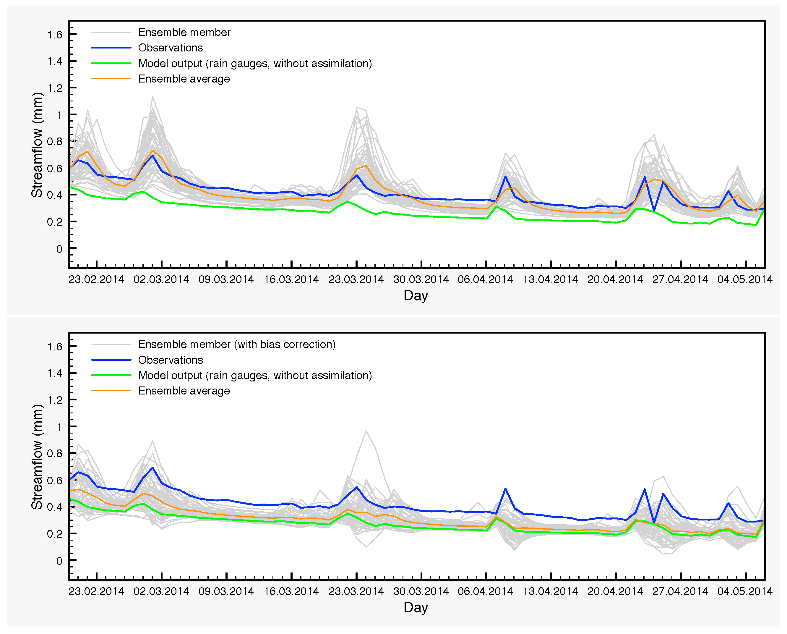
In the three-year period that we study in this article, there are cases of large differences between the control simulation and the ensemble averages for the streamflow during shorter periods of time. For example, from 20 February 2014–6 May 2014, the average of the DA ensemble is a much better approximation of the observations than the control simulation. This is clearly seen in Table 9 and in Figure 9. Of particular interest is the very large difference between the NSE coefficients. On the other hand, the average of the DA-BC ensemble is closer to the control simulation in this period with smaller errors, but still a negative NSE coefficient.
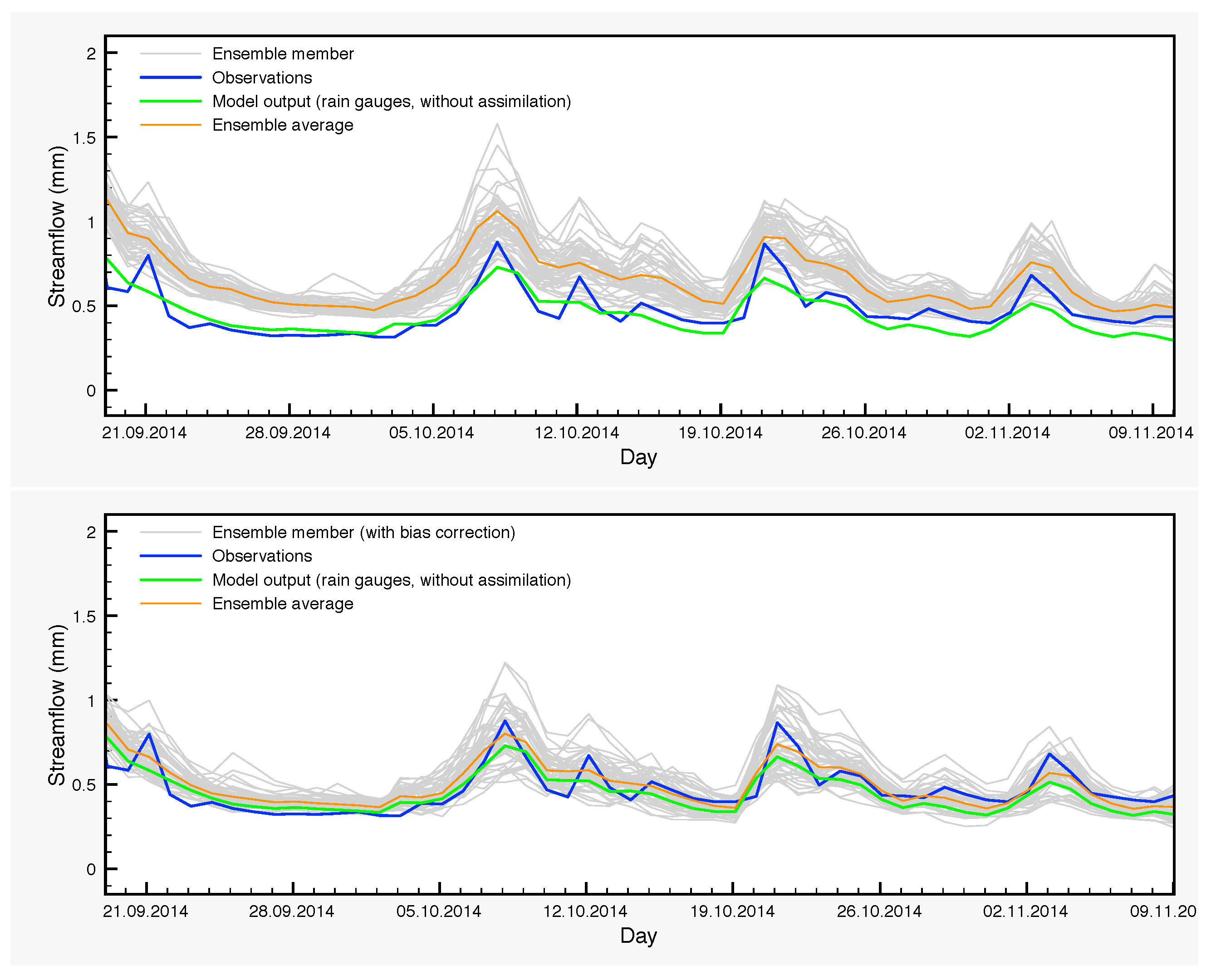
Another typical case is from 20 September 2014–10 November 2014 (Table 10 and Figure 10). Over this period, the DA ensemble average yields poor results while the scores of the control simulation appear quite normal, compared to typical SCHEME model performance. Finally, the average of the DA-BC ensemble is slightly better than the control simulation in this case.
The previous situations demonstrate the need to reduce the biases arising in EnKF where non-linear processes take place. The general idea here is to identify the sources of bias and, subsequently, to filter out their effect by running again the model while keeping active the perturbations, which are responsible for bias generation, but without assimilating any data.
It is clear also, at least for this case study, that soil moisture assimilation has a limited impact on the streamflow calculated by the model. This is not surprising because streamflow is mainly determined by precipitation. The assimilation of soil moisture would have more potential in cases where the model does not estimate correctly the water content of the soil, especially in cases with significant amounts of rainfall and saturated soils. Such indications exist also for the SCHEME model in the period that we study here. For example, we see in Figure 6 that in March 2014, there are large differences between the soil moisture values calculated by the model and detected by the satellite. The net effect of assimilating such satellite data is a slightly better streamflow output from the model (in terms of average of the DA-BC ensemble). This improvement is statistically significant, as is demonstrated in Table 6.
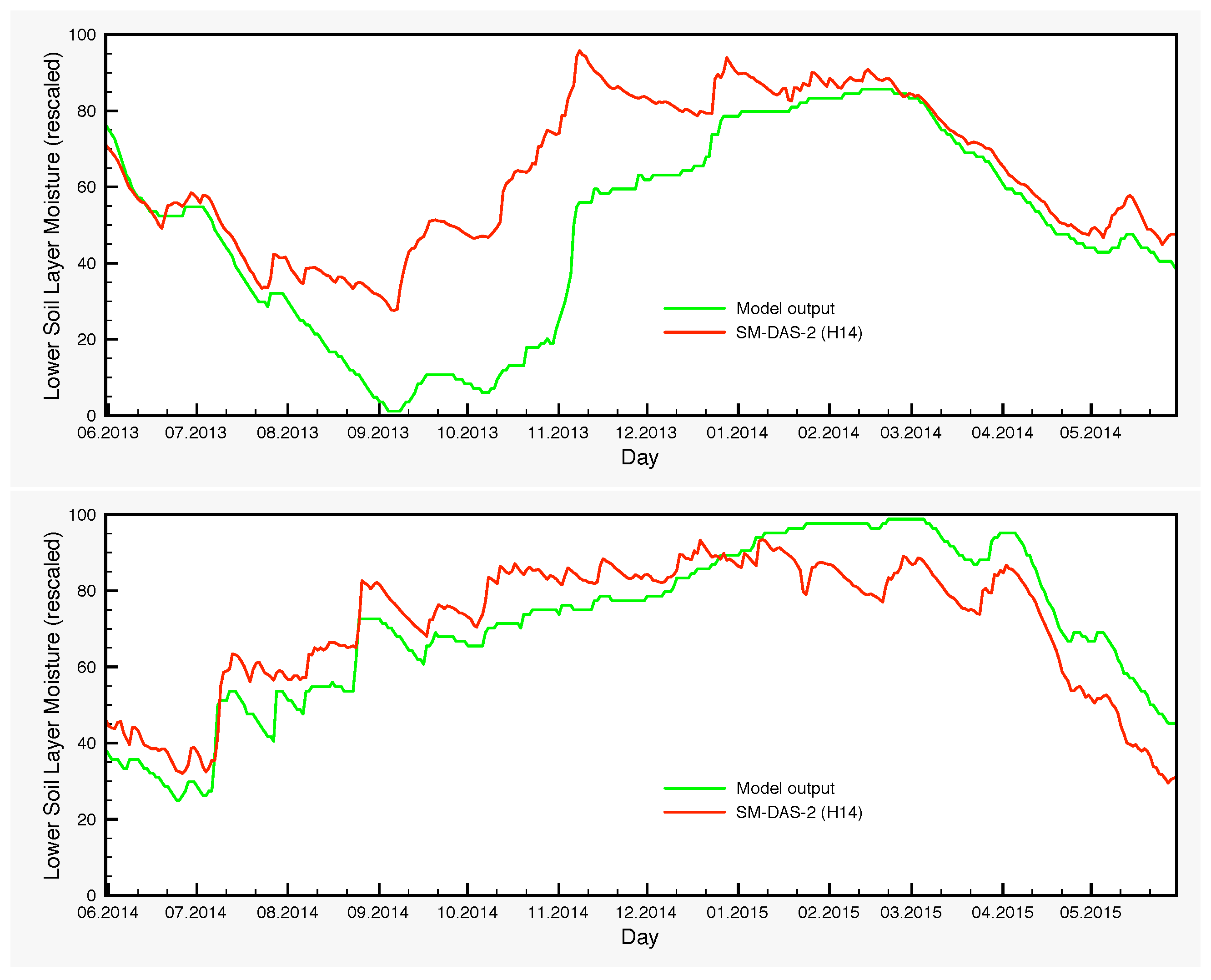
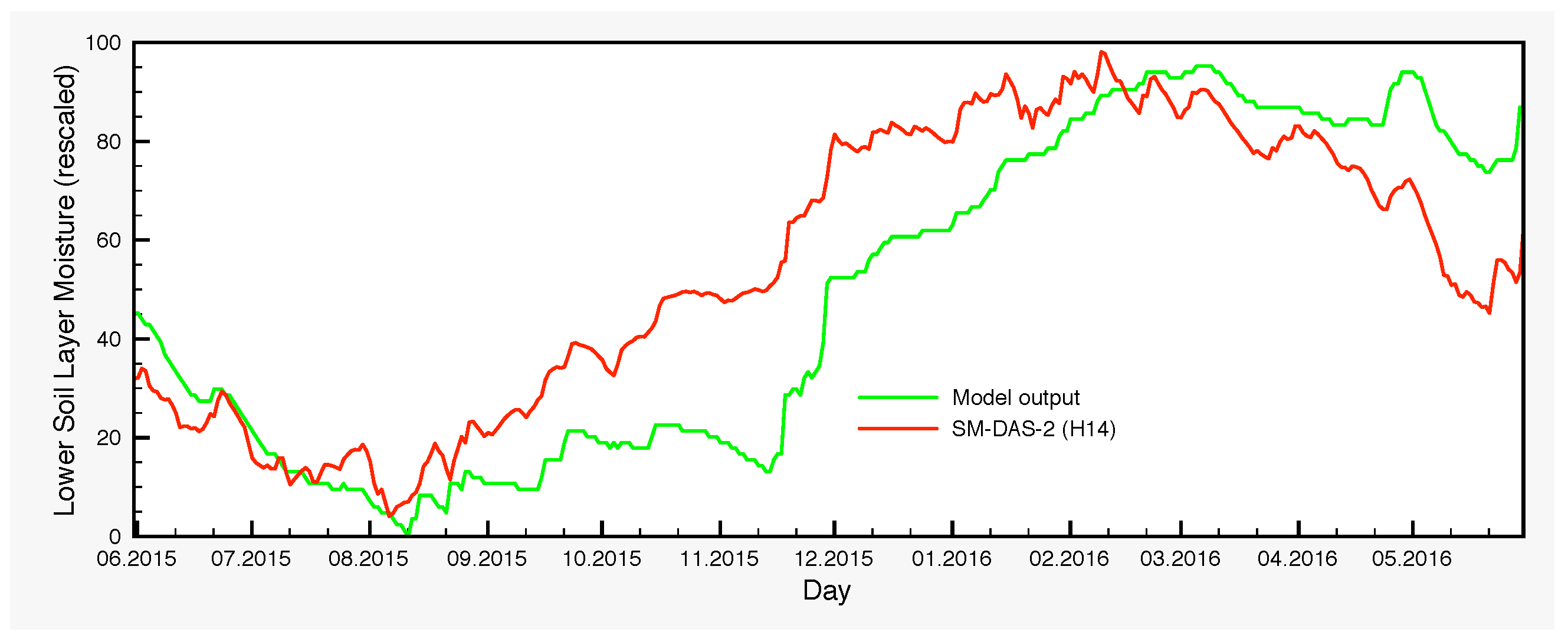
The moisture variations of the lower soil layer is another point that warrants further investigation. There are systematic differences between the control simulation and the output of the EnKF, which are larger in autumn and the beginning of winter. The origin of such deviations is in part the bias generated by the precipitation perturbations through the nonlinearities of the model and in part the assimilation itself, which transmits the satellite signal from the surface to the lower soil layer through the processes encompassed in the model, with the largest contribution coming from the latter. The lack of any soil moisture measurements for the lower layer prevents at this point a thorough analysis. However, H-SAF provides a root zone soil moisture product, SM-DAS-2 (H14). In order to compare the estimations of H14 and those of the SCHEME model, we can only rescale both in the interval [0,100], because the units are different. Therefore, no proper quantification of the differences could be made in soil moisture units. Nevertheless, visual inspection of the graphs that we provide in Figure 11 reveals striking similarities between H14 and the ensembles for the lower soil layer, generated by the SCHEME model after assimilating ASCAT SSM data (Figure 6, Figure 7 and Figure 8). This is an example where two completely different modeling approaches (the SCHEME model with EnKF for ASCAT data, on the one hand, and the ECMWF data assimilation system based on extended Kalman filter, on the other) lead to similar conclusions.
6. Conclusions
The purpose of this study is to explore the possibilities to improve streamflow estimation from a hydrological model by assimilating soil moisture data. Our analysis leads to improvements of certain aspects of the ensemble Kalman filter for bounded variables used in nonlinear processes.
The ensemble version of the Kalman filter relies on the repetitive generation of stochastic terms, which are used in order to perturb the ensemble members and calculate state corrections. In the existing literature, this leads systematically to biases, because the perturbations do not in principle preserve the bounds of a variable like the soil moisture. Here, we propose a natural solution to this problem based on truncated probability distributions, which can be applied to the case of any bounded variable.
Another problem is the generation of bias in the model output when such perturbations are applied to a variable that is used in nonlinear processes (soil moisture in our case). The solution proposed here is to identify the source of bias and to isolate its effect by running the model in ensemble mode without assimilating any data, but keeping the perturbations that cause the bias generation. The ensemble obtained in this way can be used to remove the nonlinear processes bias from the full assimilation ensemble.
The combination of the previous steps leads to very consistent data assimilation results. In summary, the streamflow estimations after data assimilation in the SCHEME hydrological model and bias correction are in many cases better than the control simulation of the model in a statistically-significant way. In the remaining situations, these estimations are statistically identical to the control.
Our results point out that the EnKF could be also used as a diagnostic tool to detect weaknesses in a model and to improve its performance. The case of March 2014 reported previously is indicative of such situations. It suggests that further investigation is required regarding the optimization of the SCHEME model parameters that control the seasonal streamflow contribution, especially in spring.
Extending the domain of hydrological simulations into other catchments will provide new insight regarding the spatial features of our data assimilation approach assisted by bias correction. Ultimately, a more extensive use of satellite data could be considered in this context.
Acknowledgments
This article is based on work supported by EUMETSAT in the framework of the H-SAF project. Discharge data are provided by the Hydrological Information Centre of the Flemish Region. Credit for the topographic data in Figure 2: U.S. Geological Survey, Department of the Interior/USGS. The authors would like to thank the reviewers and the academic editors for their constructive remarks that helped to greatly improve the manuscript.
Author Contributions
P. Baguis carried out the data processing and analysis, developed the data assimilation methodology and wrote the paper. E. Roulin proposed the main idea, offered guidance to complete the work and contributed to the editing of the manuscript and to the discussion and interpretation of the results.
Conflicts of Interest
The authors declare no conflict of interest.
Abbreviations
The following abbreviations are used in this manuscript:
| SSM | Surface Soil Moisture |
| EUMETSAT | European Organization for the Exploitation of Meteorological Satellites |
| H-SAF | Satellite Application Facility on Support to Operational Hydrology and Water Management |
| ASCAT | Advanced Scatterometer |
| MetOp | Meteorological Operational Satellites |
| EnKF | Ensemble Kalman Filter |
| SSM/I | Special Sensor Microwave Imager |
| TRMM-TMI | Tropical Rainfall Measuring Mission Microwave Imager |
| AMSR-E | Advanced Microwave Scanning Radiometer-Earth Observing System |
| NASA | National Aeronautics and Space Administration |
| SMOS | Soil Moisture and Ocean Salinity |
| ESA | European Space Agency |
| SMAP | Soil Moisture Active Passive |
| LPRM | Land Parameter Retrieval Model |
| HydroAlgo | Hydrological Algorithm |
| CDF | Cumulative Distribution Function |
| SCHEME | SCHEldt-MEuse hydrological model |
| PDM | Probability Distributed Model |
| TOPMODEL | TOPography-based hydrological MODEL |
| ANN | Artificial Neural Networks |
| ERS | European Remote-Sensing Satellite |
| IFOV | Instantaneous Field Of View |
| DA | Data Assimilation |
| DA-BC | Data Assimilation and Bias Correction |
| A-Bias | Absolute Bias |
| RMSE | Root Mean Square Error |
| NSE | Nash–Sutcliffe Efficiency coefficient |
References
- Dorigo, W.A.; Wagner, W.; Hohensinn, R.; Hahn, S.; Paulik, C.; Xaver, A.; Gruber, A.; Drusch, M.; Mecklenburg, S.; van Oevelen, P.; et al. The International Soil Moisture Network: A data hosting facility for global in situ soil moisture measurements. Hydrol. Earth Syst. Sci. 2011, 15, 1675–1698. [Google Scholar] [CrossRef]
- Albergel, C.; de Rosnay, P.; Balsamo, G.; Isaksen, L.; Muñoz-Sabater, J. Soil Moisture Analyses at ECMWF: Evaluation Using Global Ground-Based In Situ Observations. J. Hydrometeorol. 2012, 13, 1442–1460. [Google Scholar] [CrossRef]
- Njoku, E.; Chan, S. Vegetation and surface roughness effects on AMSR-E land observations. Remote Sens. Environ. 2006, 100, 190–199. [Google Scholar] [CrossRef]
- Koike, T.; Nakamura, Y.; Kaihotsu, I.; Davva, G.; Matsuura, N.; Tamagawa, K.; Fujii, H. Development of an Advanced Microwave Scanning Radiometer (AMSR-E) algorithm of soil moisture and vegetation water content. Annu. J. Hydraul. Eng. Jpn. Soc. Civ. Eng. 2004, 48, 217–222. [Google Scholar] [CrossRef]
- Kerr, Y.; Waldteufel, P.; Richaume, P.; Wigneron, J.-P.; Ferrazzoli, P.; Mahmoodi, A.; Al Bitar, A.; Cabot, F.; Gruhier, C.; Juglea, S.; et al. The SMOS soil moisture retrieval algorithm. IEEE Trans. Geosci. Remote Sens. 2012, 50, 1384–1403. [Google Scholar] [CrossRef]
- Entekhabi, D.; Njoku, E.G.; O’Neill, P.E.; Kellogg, K.H.; Crow, W.T.; Edelstein, W.N.; Entin, J.K.; Goodman, S.D.; Jackson, T.J.; Johnson, J.; et al. The Soil Moisture Active and Passive (SMAP) mission. Proc. IEEE 2010, 98, 704–716. [Google Scholar] [CrossRef]
- Bartalis, Z.; Wagner, W.; Naeimi, V.; Hasenauer, S.; Scipal, K.; Bonekamp, H.; Figa, J.; Anderson, C. Initial soil moisture retrievals from the METOP-A Advanced Scatterometer (ASCAT). Geophys. Res. Lett. 2007, 34, L20401. [Google Scholar] [CrossRef]
- Owe, M.; de Jeu, R.; Holmes, T. Multisensor historical climatology of satellite-derived global land surface moisture. J. Geophys. Res. 2008, 113, F01002. [Google Scholar] [CrossRef]
- Santi, E.; Pettinato, S.; Paloscia, S.; Pampaloni, P.; Macelloni, G.; Brogioni, M. An algorithm for generating soil moisture and snow depth maps from microwave spaceborne radiometers: HydroAlgo. Hydrol. Earth Syst. Sci. 2012, 16, 3659–3676. [Google Scholar] [CrossRef]
- Wanders, N.; Karssenberg, D.; de Roo, A.; de Jong, S.M.; Bierkens, M.F.P. The suitability of remotely sensed soil moisture for improving operational flood forecasting. Hydrol. Earth Syst. Sci. 2014, 18, 2343–2357. [Google Scholar] [CrossRef]
- Alvarez-Garreton, C.; Ryu, D.; Western, A.W.; Su, C.-H.; Crow, W.T.; Robertson, D.E.; Leahy, C. Improving operational flood ensemble prediction by the assimilation of satellite soil moisture: Comparison between lumped and semi-distributed schemes. Hydrol. Earth Syst. Sci. 2015, 19, 1659–1676. [Google Scholar] [CrossRef]
- Brocca, L.; Moramarco, T.; Melone, F.; Wagner, W.; Hasenauer, S.; Hahn, S. Assimilation of Surface- and Root-Zone ASCAT Soil Moisture Products Into Rainfall-Runoff Modeling. IEEE Trans. Geosci. Remote Sens. 2012, 50, 2542–2555. [Google Scholar] [CrossRef]
- Chen, F.; Crow, W.T.; Starks, P.J.; Moriasi, D.N. Improving hydrologic predictions of a catchment model via assimilation of surface soil moisture. Adv. Water Resour. 2011, 34, 526–536. [Google Scholar] [CrossRef]
- Brocca, L.; Melone, F.; Moramarco, T.; Wagner, W.; Naeimi, V.; Bartalis, Z.; Hasenauer, S. Improving runoff prediction through the assimilation of the ASCAT soil moisture product. Hydrol. Earth Syst. Sci. 2010, 14, 1881–1893. [Google Scholar] [CrossRef]
- Pauwels, V.R.N.; Hoeben, R.; Verhoest, N.E.C.; De Troch, F.P.; Troch, P.A. Improvement of TOPLATS-based discharge predictions through assimilation of ERS-based remotely sensed soil moisture values. Hydrol. Processes 2002, 16, 995–1013. [Google Scholar] [CrossRef]
- Massari, C.; Brocca, L.; Ciabatta, L.; Moramarco, T.; Gabellani, S.; Albergel, C.; De Rosnay, P.; Puca, S.; Wagner, W. The Use of H-SAF Soil Moisture Products for Operational Hydrology: Flood Modelling over Italy. Hydrology 2015, 2, 2–22. [Google Scholar] [CrossRef]
- Crow, W.; Bindlish, R.; Jackson, T. The added value of spaceborne passive microwave soil moisture retrievals for forecasting rainfall–runoff partitioning. Geophys. Res. Lett. 2005, 32, L18401. [Google Scholar] [CrossRef]
- Jackson, T.J.; Cosh, M.H.; Bindlish, R.; Starks, P.J.; Bosch, D.D.; Seyfried, M.; Goodrich, D.C.; Moran, M.S.; Du, J. Validation of Advanced Microwave Scanning Radiometer Soil Moisture Products. IEEE Trans. Geosci. Remote Sens. 2010, 48, 4256–4272. [Google Scholar] [CrossRef]
- Reichle, R.H.; Koster, R.D. Bias reduction in short records of satellite soil moisture. Geophys. Res. Lett. 2004, 31, L19501. [Google Scholar] [CrossRef]
- Matgen, P.; Heitz, S.; Hasenauer, S.; Hissler, C.; Brocca, L.; Hoffmann, L.; Wagner, W.; Savenije, H.H.G. On the potential of MetOp ASCAT-derived soil wetness indices as a new aperture for hydrological monitoring and prediction: A field evaluation over Luxembourg. Hydrol. Process. 2012, 26, 2346–2359. [Google Scholar]
- Alvarez-Garreton, C.; Ryu, D.; Western, A.W.; Crow, W.T.; Robertson, D.E. The impacts of assimilating satellite soil moisture into a rainfall-runoff model in a semi-arid catchment. J. Hydrol. 2014, 519, 2763–2774. [Google Scholar] [CrossRef]
- Brocca, L.; Hasenauer, S.; Lacava, T.; Melone, F.; Moramarco, T.; Wagner, W.; Dorigo, W.; Matgen, P.; Martínez-Fernández, J.; Llorens, P.; et al. Soil moisture estimation through ASCAT and AMSR-E sensors: An intercomparison and validation study across Europe. Remote Sens. Environ. 2011, 115, 3390–3408. [Google Scholar] [CrossRef]
- Dorigo, W.A.; Scipal, K.; Parinussa, R.M.; Liu, Y.Y.; Wagner, W.; de Jeu, R.A.M.; Naeimi, V. Error characterisation of global active and passive microwave soil moisture datasets. Hydrol. Earth Syst. Sci. 2010, 14, 2605–2616. [Google Scholar] [CrossRef] [Green Version]
- Su, C.-H.; Ryu, D.; Western, A.W.; Wagner, W. De-noising of passive and active microwave satellite soil moisture time series. Geophys. Res. Lett. 2013, 40, 3624–3630. [Google Scholar] [CrossRef]
- Massari, C.; Brocca, L.; Tarpanelli, A.; Moramarco, T. Data Assimilation of Satellite Soil Moisture into Rainfall-Runoff Modelling: A Complex Recipe? Remote Sens. 2015, 7, 11403–11433. [Google Scholar] [CrossRef]
- Evensen, G. The Ensemble Kalman Filter: Theoretical formulation and practical implementation. Ocean Dyn. 2003, 53, 343–367. [Google Scholar] [CrossRef]
- Burgers, G.; van Leeuwen, P.J.; Evensen, G. Analysis Scheme in the Ensemble Kalman Filter. Mon. Weather Rev. 1998, 126, 1719–1724. [Google Scholar] [CrossRef]
- Reichle, R.H.; McLaughlin, D.B.; Entekhabi, D. Hydrologic Data Assimilation with the Ensemble Kalman Filter. Mon. Weather Rev. 2002, 130, 103–114. [Google Scholar] [CrossRef]
- Kalman, R.E. A new approach to linear filtering and prediction problems. J. Basic Eng. 1960, 82, 35–45. [Google Scholar] [CrossRef]
- De Lannoy, G.J.M.; Houser, P.R.; Pauwels, V.R.N.; Verhoest, N.E.C. Assessment of model uncertainty for soil moisture through ensemble verification. J. Geophys. Res. 2006, 111, 1–18. [Google Scholar] [CrossRef]
- Ryu, D.; Crow, W.T.; Zhan, X.; Jackson, T.J. Correcting Unintended Perturbation Biases in Hydrologic Data Assimilation. J. Hydrometeorol. 2009, 10, 734–750. [Google Scholar] [CrossRef]
- De Lannoy, G.J.M.; Reichle, R.H.; Houser, P.R.; Pauwels, V.R.N.; Verhoest, N.E.C. Correcting for forecast bias in soil moisture assimilation with the Ensemble Kalman filter. Water Resour. Res. 2007, 43, W09410. [Google Scholar] [CrossRef]
- Turner, M.R.J.; Walker, J.P.; Oke, P.R. Ensemble member generation for sequential data assimilation. Remote Sens. Environ. 2008, 112, 1421–1433. [Google Scholar] [CrossRef]
- Wagner, W.; Lemoine, G.; Borgeaud, M.; Rott, H. A study of vegetation cover effects on ERS scatterometer data. IEEE Trans. Geosci. Remote Sens. 1999, 37, 938–948. [Google Scholar] [CrossRef]
- Albergel, C.; Rüdiger, C.; Carrer, D.; Calvet, J.-C.; Fritz, N.; Naeimi, V.; Bartalis, Z.; Hasenauer, S. An evaluation of ASCAT surface soil moisture products with in situ observations in Southwestern France. Hydrol. Earth Syst. Sci. 2009, 13, 115–124. [Google Scholar] [CrossRef]
- Brocca, L.; Crow, W.T.; Ciabatta, L.; Massari, C.; de Rosnay, P.; Enenkel, M.; Hahn, S.; Amarnath, G.; Camici, S.; Tarpanelli, A.; et al. A Review of the Applications of ASCAT Soil Moisture Products. IEEE J. Sel. Top. Appl. Earth Obs. Remote Sens. 2017, 10, 2285–2306. [Google Scholar] [CrossRef]
- Paulik, C.; Dorigo, W.; Wagner, W.; Kidd, R. Validation of the ASCAT Soil Water Index using in situ data from the International Soil Moisture Network. Int. J. Appl. Earth Obs. Geoinf. 2014, 30, 1–18. [Google Scholar] [CrossRef]
- Bultot, F.; Dupriez, G. Conceptual hydrological model for an average-sized catchment area. J. Hydrol. 1976, 29, 251–292. [Google Scholar] [CrossRef]
- Gellens, D.; Roulin, E. Streamflow response of Belgian catchments to IPCC climate change scenarios. J. Hydrol. 1998, 210, 242–258. [Google Scholar] [CrossRef]
- Bultot, F.; Coppens, A.; Dupriez, G.; Gellens, D.; Meulenberghs, F. Repercussions of a CO2 doubling on the water cycle and on the water balance—A case study for Belgium. J. Hydrol. 1988, 99, 319–347. [Google Scholar] [CrossRef]
- Bultot, F.; Gellens, D.; Spreafico, M.; Schädler, B. Repercussions of a CO2 doubling on the water balance—A case study in Switzerland. J. Hydrol. 1992, 137, 199–208. [Google Scholar] [CrossRef]
- Gellens, D.; Barbieux, K.; Schädler, B.; Roulin, E.; Aschwanden, H.; Gellens-Meulenberghs, F. Snow Cover Modelling as a Tool for Climate Change Assessment in a Swiss Alpine Catchment. Hydrol. Res. 2000, 31, 73–88. [Google Scholar]
- Roulin, E.; Vannitsem, S. Skill of medium-range hydrological ensemble predictions. J. Hydrometeorol. 2005, 6, 729–744. [Google Scholar] [CrossRef]
- Van den Bergh, J.; Roulin, E. Postprocessing of Medium Range Hydrological Ensemble Forecasts Making Use of Reforecasts. Hydrology 2016, 3, 21. [Google Scholar] [CrossRef]
- Naden, P.S. Spatial variability in flood estimation for large catchments: The exploitation of channel network structure. Hydrol. Sci. J. 1992, 37, 53–71. [Google Scholar] [CrossRef]
- Moore, R.J. The PDM rainfall-runoff model. Hydrol. Earth Syst. Sci. 2007, 11, 483–499. [Google Scholar] [CrossRef]
- Duan, Q.; Sorooshian, S.; Gupta, V.K. Effective and efficient global optimization for conceptual rainfall-runoff models. Water Resour. Res. 1992, 28, 1015–1031. [Google Scholar] [CrossRef]
- Duan, Q.; Sorooshian, S.; Gupta, V.K. Optimal use of the SCE-UA global optimisation method for calibrating watershed models. J. Hydrol. 1994, 158, 265–284. [Google Scholar] [CrossRef]
- Goodman, P.; Harrell, F.E. Neural Networks: Advantages and Limitations for Statistical Modeling. In Proceedings of the Biometrics Section, Joint Statistical Meeting, American Statistical Association, Alexandria, VA, USA, 8–10 August 1998. [Google Scholar]
- European Communities (EC). Soil Map of the European Communities at 1:1,000,000; EC: Luxembourg, 1985; p. 124. [Google Scholar]
- Efron, B.; Tibshirani, R. An Introduction to the Bootstrap; Chapman & Hall, Inc.: New York, NY, USA, 1993; ISBN 0412042312. [Google Scholar]
- Johnson, N.L.; Kotz, S.; Balakrishnan, N. Continuous Univariate Distributions, 2nd ed.; John Wiley: New York, NY, USA, 1994; Volume 1, ISBN 0471584959. [Google Scholar]
- Paris Anguela, T.; Zribi, M.; Hasenauer, S.; Habets, F.; Loumagne, C. Analysis of surface and root-zone soil moisture dynamics with ERS scatterometer and the hydrometeorological model SAFRAN-ISBA-MODCOU at Grand Morin watershed (France). Hydrol. Earth Syst. Sci. 2008, 12, 1415–1424. [Google Scholar] [CrossRef] [Green Version]
- Naeimi, V.; Scipal, K.; Bartalis, Z.; Hasenauer, S.; Wagner, W. An Improved Soil Moisture Retrieval Algorithm for ERS and METOP Scatterometer Observations. IEEE Trans. Geosci. Remote Sens. 2009, 47, 1999–2013. [Google Scholar] [CrossRef]
- De Rosnay, P.; Drusch, M.; Vasiljevic, D.; Balsamo, G.; Albergel, C.; Isaksen, L. A simplified Extended Kalman Filter for the global operational soil moisture analysis at ECMWF. Q. J. R. Meteorol. Soc. 2013, 139, 1199–1213. [Google Scholar] [CrossRef]
- Balsamo, G.; Albergel, C.; Beljaars, A.; Boussetta, S.; Brun, E.; Cloke, H.; Dee, D.; Dutra, E.; Pappenberger, F.; de Rosnay, P.; et al. ERA-Interim/Land: A Global Land-Surface Reanalysis Based on ERA-Interim Meteorological Forcing; ERA Report Series; ECMWF: Reading, UK, 2012; Volume 13, pp. 1–25. [Google Scholar]
Figure 1.
Diagram of the SCHEME model. Model parameters: (1) , threshold value for upper soil reservoir; (2) scr(4), seasonal runoff coefficients; (3) , redirection coefficient for surface flow; (4) a, b and c, parameters describing a unit hydrograph; (5) and , recession coefficients of the underground reservoirs; (6) v and D, routing module parameters.

Figure 2.
Left panel: The Meuse and the Scheldt River Basins, including the Demer catchment. Right panel: Topographic details and elevation data in meters in the Demer catchment. The small red square is the catchment outlet.
Figure 2.
Left panel: The Meuse and the Scheldt River Basins, including the Demer catchment. Right panel: Topographic details and elevation data in meters in the Demer catchment. The small red square is the catchment outlet.

Figure 3.
Bias for the surface soil moisture product H07, based on data from June 2009–May 2013. The original raw data are also shown.
Figure 3.
Bias for the surface soil moisture product H07, based on data from June 2009–May 2013. The original raw data are also shown.
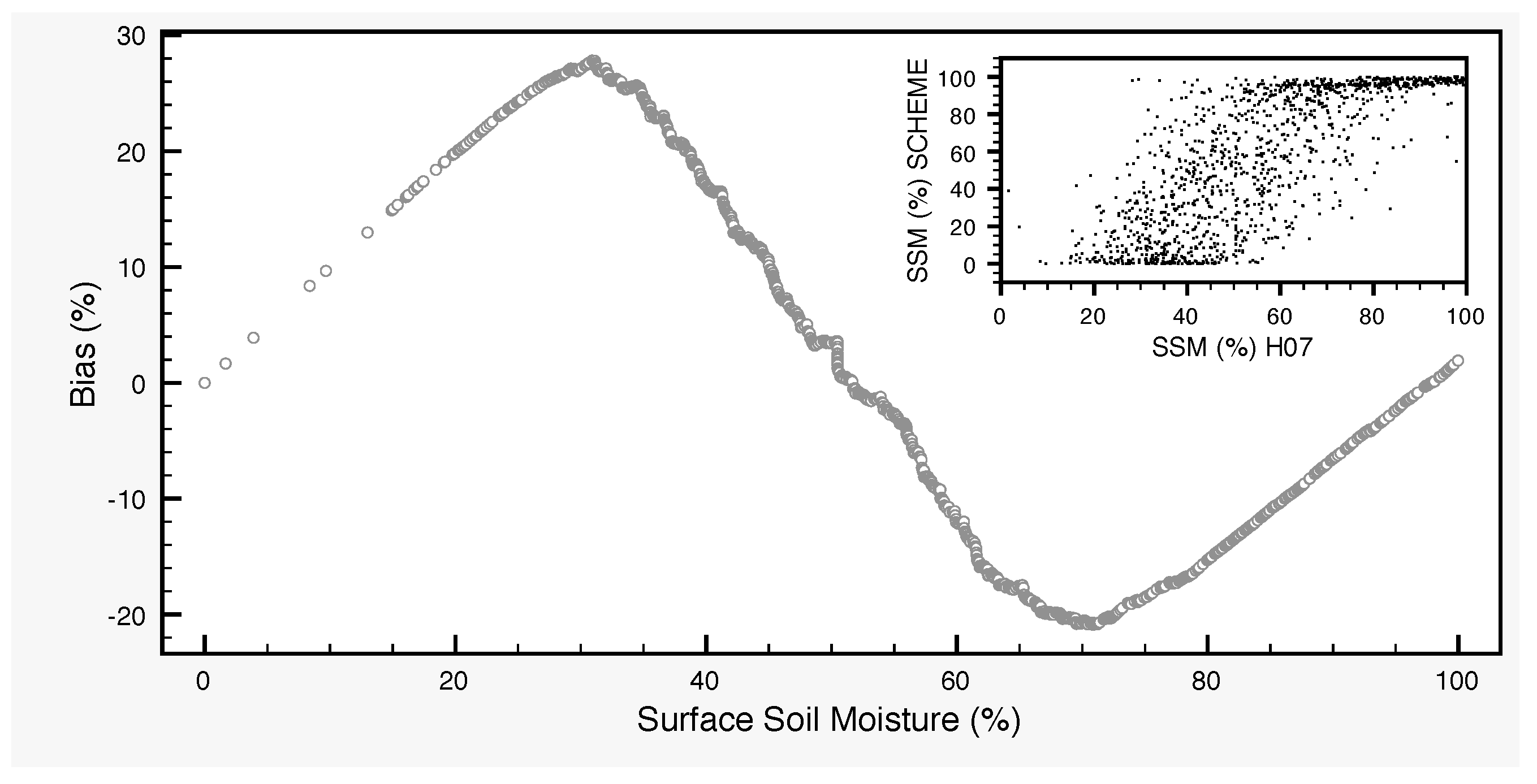
Figure 4.
Probability distribution of surface soil moisture values, based on simulation data with the SCHEME model, from January 1966–December 1995. The bins subdivide the interval formed by the whole dataset into ten equal parts.
Figure 4.
Probability distribution of surface soil moisture values, based on simulation data with the SCHEME model, from January 1966–December 1995. The bins subdivide the interval formed by the whole dataset into ten equal parts.

Figure 5.
Probability distribution of surface soil moisture standard deviation values, based on simulation data with the SCHEME model, from January 1966–December 1995. The bins subdivide the standard deviation intervals corresponding to each soil moisture class into ten equal parts.
Figure 5.
Probability distribution of surface soil moisture standard deviation values, based on simulation data with the SCHEME model, from January 1966–December 1995. The bins subdivide the standard deviation intervals corresponding to each soil moisture class into ten equal parts.

Figure 6.
Hydrological data and model output for the period June 2013–May 2014. From top to bottom: precipitation, soil moisture in the upper layer, soil moisture in the lower layer, streamflow with data assimilation only and streamflow with data assimilation and bias correction.
Figure 6.
Hydrological data and model output for the period June 2013–May 2014. From top to bottom: precipitation, soil moisture in the upper layer, soil moisture in the lower layer, streamflow with data assimilation only and streamflow with data assimilation and bias correction.
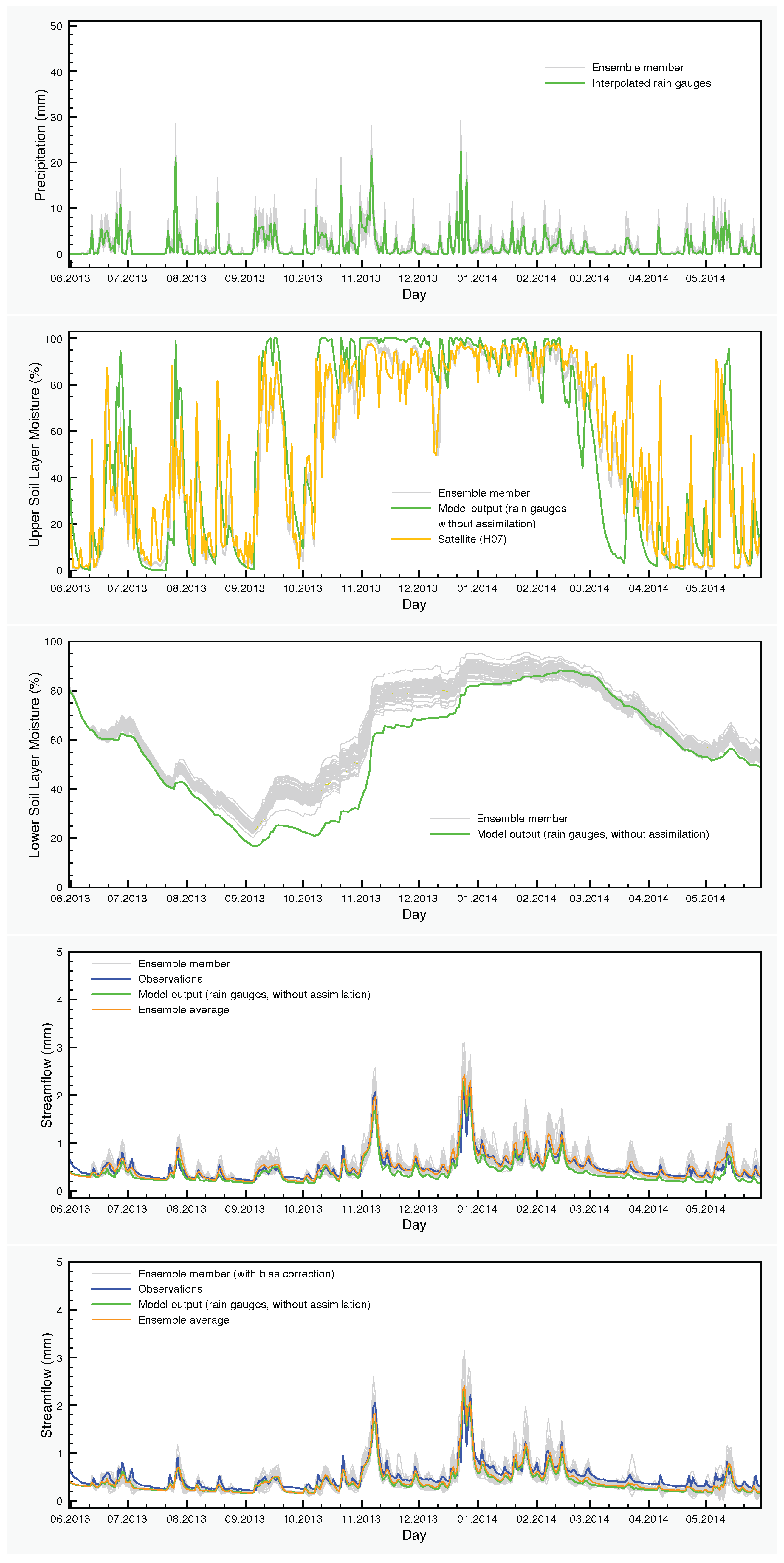
Figure 7.
Hydrological data and model output for the period June 2014–May 2015. From top to bottom: precipitation, soil moisture in the upper layer, soil moisture in the lower layer, streamflow with data assimilation only and streamflow with data assimilation and bias correction.
Figure 7.
Hydrological data and model output for the period June 2014–May 2015. From top to bottom: precipitation, soil moisture in the upper layer, soil moisture in the lower layer, streamflow with data assimilation only and streamflow with data assimilation and bias correction.

Figure 8.
Hydrological data and model output for the period June 2015–May 2016. From top to bottom: precipitation, soil moisture in the upper layer, soil moisture in the lower layer, streamflow with data assimilation only and streamflow with data assimilation and bias correction.
Figure 8.
Hydrological data and model output for the period June 2015–May 2016. From top to bottom: precipitation, soil moisture in the upper layer, soil moisture in the lower layer, streamflow with data assimilation only and streamflow with data assimilation and bias correction.
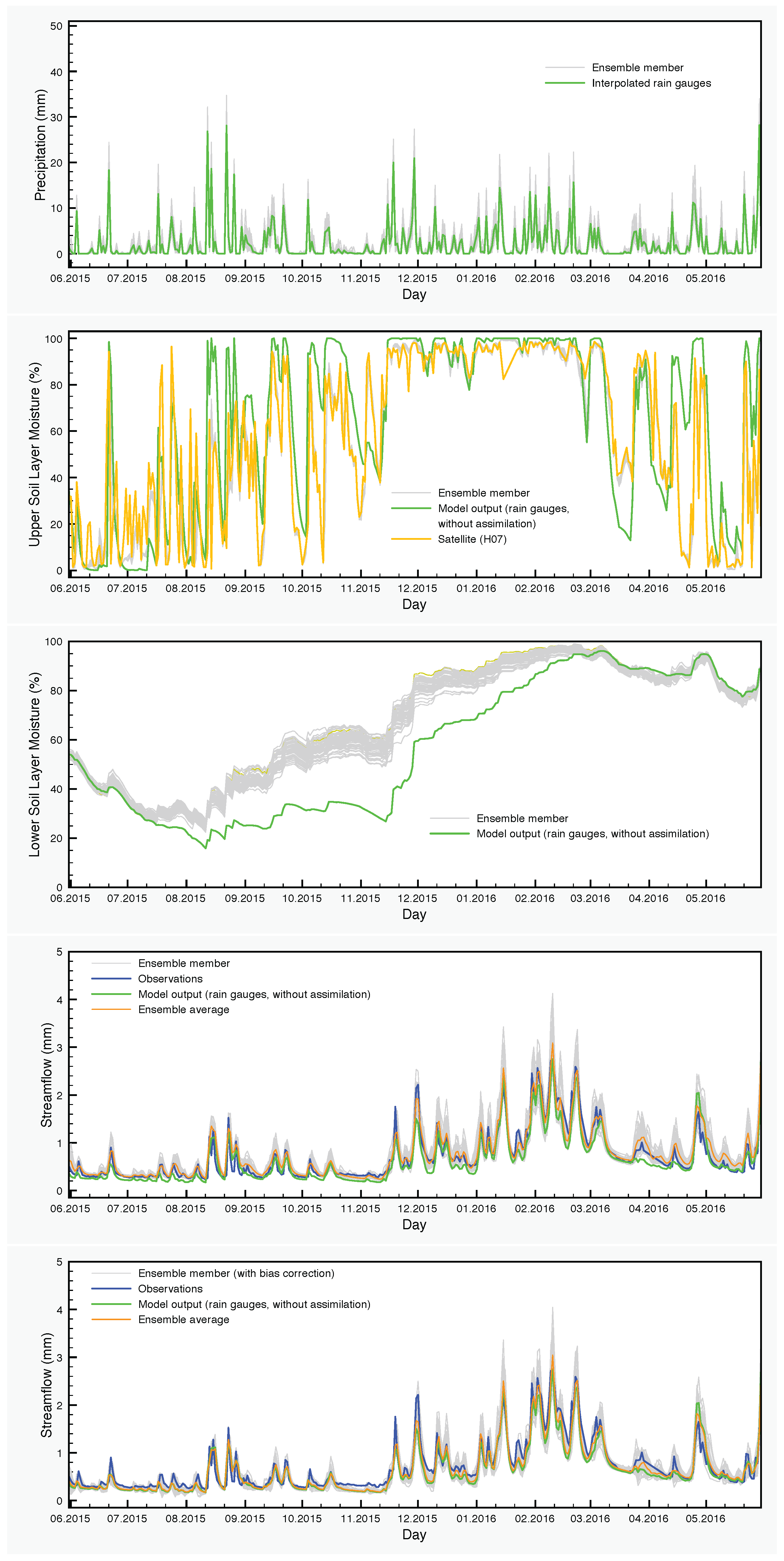
Figure 9.
Streamflow for the period 20 February 2014–6 May 2014.

Figure 10.
Streamflow for the period 20 September 2014–10 November 2014.

Figure 11.
Areal average for the lower soil layer moisture of the SCHEME model and the H-SAF product H14, over three successive years (1 June 2013–31 May 2016). The SCHEME model output is given originally as the degree of saturation (%), while H14 is in volumetric units (m3/m3). A rescaling has been applied in both time series for this comparison.

Table 1.
Synoptic statistics for streamflow with and without bias correction in the ensemble, 1 June 2013–31 May 2016. The unit for bias, Absolute bias (A-bias) and RMSE is .
Table 1.
Synoptic statistics for streamflow with and without bias correction in the ensemble, 1 June 2013–31 May 2016. The unit for bias, Absolute bias (A-bias) and RMSE is .
| Bias | A-Bias | RMSE | R | NSE | |
|---|---|---|---|---|---|
| Reference simulation | −0.077 | 0.130 | 0.176 | 0.938 | 0.848 |
| Ensemble mean DA | 0.062 | 0.111 | 0.171 | 0.943 | 0.856 |
| Ensemble mean DA-BC | −0.039 | 0.114 | 0.159 | 0.946 | 0.876 |
Table 2.
Synoptic statistics for streamflow with and without bias correction in the ensemble, 1 June 2013–31 May 2014. The unit for bias, A-bias and RMSE is .
Table 2.
Synoptic statistics for streamflow with and without bias correction in the ensemble, 1 June 2013–31 May 2014. The unit for bias, A-bias and RMSE is .
| Bias | A-Bias | RMSE | R | NSE | |
|---|---|---|---|---|---|
| Reference simulation | |||||
| Annual | −0.094 | 0.116 | 0.138 | 0.940 | 0.769 |
| Summer 2013 | −0.074 | 0.087 | 0.107 | 0.817 | 0.359 |
| Autumn 2013 | −0.075 | 0.096 | 0.119 | 0.958 | 0.856 |
| Winter 2013–2014 | −0.101 | 0.147 | 0.170 | 0.946 | 0.763 |
| Spring 2014 | −0.126 | 0.136 | 0.147 | 0.706 | −1.310 |
| Ensemble mean DA | |||||
| Annual | 0.017 | 0.068 | 0.105 | 0.952 | 0.866 |
| Summer 2013 | −0.020 | 0.059 | 0.090 | 0.788 | 0.539 |
| Autumn 2013 | 0.017 | 0.062 | 0.077 | 0.971 | 0.939 |
| Winter 2013–2014 | 0.056 | 0.087 | 0.141 | 0.959 | 0.836 |
| Spring 2014 | 0.019 | 0.065 | 0.099 | 0.764 | −0.060 |
| Ensemble mean DA-BC | |||||
| Annual | −0.068 | 0.099 | 0.121 | 0.947 | 0.821 |
| Summer 2013 | −0.075 | 0.089 | 0.109 | 0.808 | 0.332 |
| Autumn 2013 | −0.053 | 0.078 | 0.094 | 0.968 | 0.909 |
| Winter 2013–2014 | −0.043 | 0.117 | 0.150 | 0.945 | 0.816 |
| Spring 2014 | −0.100 | 0.111 | 0.125 | 0.721 | −0.672 |
Table 3.
Synoptic statistics for streamflow with and without bias correction in the ensemble, 1 June 2014–31 May 2015. The unit for bias, A-bias and RMSE is .
Table 3.
Synoptic statistics for streamflow with and without bias correction in the ensemble, 1 June 2014–31 May 2015. The unit for bias, A-bias and RMSE is .
| Bias | A-Bias | RMSE | R | NSE | |
|---|---|---|---|---|---|
| Reference simulation | |||||
| Annual | −0.052 | 0.133 | 0.192 | 0.927 | 0.831 |
| Summer 2014 | 0.001 | 0.165 | 0.239 | 0.930 | 0.739 |
| Autumn 2014 | −0.043 | 0.091 | 0.126 | 0.758 | 0.508 |
| Winter 2014–2015 | −0.054 | 0.158 | 0.215 | 0.926 | 0.840 |
| Spring 2015 | −0.109 | 0.119 | 0.167 | 0.928 | 0.729 |
| Ensemble mean DA | |||||
| Annual | 0.102 | 0.149 | 0.224 | 0.920 | 0.770 |
| Summer 2014 | 0.189 | 0.208 | 0.326 | 0.935 | 0.512 |
| Autumn 2014 | 0.145 | 0.156 | 0.185 | 0.786 | −0.056 |
| Winter 2014–2015 | 0.035 | 0.146 | 0.212 | 0.929 | 0.846 |
| Spring 2015 | 0.038 | 0.085 | 0.121 | 0.935 | 0.857 |
| Ensemble mean DA-BC | |||||
| Annual | −0.005 | 0.125 | 0.189 | 0.930 | 0.837 |
| Summer 2014 | 0.036 | 0.170 | 0.252 | 0.932 | 0.707 |
| Autumn 2014 | 0.007 | 0.079 | 0.111 | 0.791 | 0.623 |
| Winter 2014–2015 | 0.007 | 0.153 | 0.216 | 0.925 | 0.839 |
| Spring 2015 | −0.073 | 0.097 | 0.141 | 0.927 | 0.806 |
Table 4.
Synoptic statistics for streamflow with and without bias correction in the ensemble, 1 June 2015–31 May 2016. The unit for bias, A-bias and RMSE is .
Table 4.
Synoptic statistics for streamflow with and without bias correction in the ensemble, 1 June 2015–31 May 2016. The unit for bias, A-bias and RMSE is .
| Bias | A-Bias | RMSE | R | NSE | |
|---|---|---|---|---|---|
| Reference simulation | |||||
| Annual | −0.084 | 0.141 | 0.193 | 0.944 | 0.867 |
| Summer 2015 | −0.043 | 0.125 | 0.160 | 0.777 | 0.461 |
| Autumn 2015 | −0.074 | 0.094 | 0.125 | 0.886 | 0.667 |
| Winter 2015–2016 | −0.195 | 0.221 | 0.272 | 0.950 | 0.802 |
| Spring 2016 | −0.019 | 0.125 | 0.184 | 0.909 | 0.773 |
| Ensemble mean DA | |||||
| Annual | 0.065 | 0.116 | 0.164 | 0.959 | 0.904 |
| Summer 2015 | 0.083 | 0.099 | 0.166 | 0.826 | 0.413 |
| Autumn 2015 | 0.038 | 0.081 | 0.113 | 0.881 | 0.729 |
| Winter 2015–2016 | 0.006 | 0.137 | 0.177 | 0.958 | 0.917 |
| Spring 2016 | 0.140 | 0.151 | 0.190 | 0.949 | 0.758 |
| Ensemble mean DA-BC | |||||
| Annual | −0.045 | 0.118 | 0.160 | 0.957 | 0.909 |
| Summer 2015 | −0.035 | 0.116 | 0.154 | 0.780 | 0.498 |
| Autumn 2015 | −0.059 | 0.089 | 0.117 | 0.889 | 0.711 |
| Winter 2015–2016 | −0.103 | 0.169 | 0.210 | 0.956 | 0.883 |
| Spring 2016 | 0.021 | 0.096 | 0.143 | 0.939 | 0.862 |
Table 5.
Statistical significance of the differences between the scores of the ensemble averages and the corresponding scores of the reference simulation for streamflow, 1 June 2013–31 May 2016.
Table 5.
Statistical significance of the differences between the scores of the ensemble averages and the corresponding scores of the reference simulation for streamflow, 1 June 2013–31 May 2016.
| Bias | A-Bias | RMSE | R | NSE | |
|---|---|---|---|---|---|
| Ensemble mean DA | Y+ | Y+ | N | N | N |
| Ensemble mean DA-BC | Y+ | Y+ | Y+ | N | Y+ |
Table 6.
Statistical significance of the differences between the scores of the ensemble averages and the corresponding scores of the reference simulation for streamflow, 1 June 2013–31 May 2014.
Table 6.
Statistical significance of the differences between the scores of the ensemble averages and the corresponding scores of the reference simulation for streamflow, 1 June 2013–31 May 2014.
| Bias | A-Bias | RMSE | R | NSE | |
|---|---|---|---|---|---|
| Ensemble mean DA | |||||
| Annual | Y+ | Y+ | Y+ | N | Y+ |
| Summer 2013 | Y+ | Y+ | N | N | N |
| Autumn 2013 | Y+ | Y+ | Y+ | N | N |
| Winter 2013–2014 | Y+ | Y+ | N | N | N |
| Spring 2014 | Y+ | Y+ | Y+ | N | Y+ |
| Ensemble mean DA-BC | |||||
| Annual | Y+ | Y+ | Y+ | N | N |
| Summer 2013 | N | N | N | N | N |
| Autumn 2013 | Y+ | Y+ | Y+ | N | N |
| Winter 2013–2014 | Y+ | Y+ | N | N | N |
| Spring 2014 | Y+ | Y+ | Y+ | N | N |
Table 7.
Statistical significance of the differences between the scores of the ensemble averages and the corresponding scores of the reference simulation for streamflow, 1 June 2014–31 May 2015.
Table 7.
Statistical significance of the differences between the scores of the ensemble averages and the corresponding scores of the reference simulation for streamflow, 1 June 2014–31 May 2015.
| Bias | A-Bias | RMSE | R | NSE | |
|---|---|---|---|---|---|
| Ensemble mean DA | |||||
| Annual | Y- | N | Y- | N | Y- |
| Summer 2014 | Y- | N | N | N | Y- |
| Autumn 2014 | Y- | Y- | Y- | N | Y- |
| Winter 2014–2015 | Y+ | N | N | N | N |
| Spring 2015 | Y+ | Y+ | Y+ | N | Y+ |
| Ensemble mean DA-BC | |||||
| Annual | Y+ | N | N | N | N |
| Summer 2014 | N | N | N | N | N |
| Autumn 2014 | Y+ | N | N | N | N |
| Winter 2014–2015 | Y+ | N | N | N | N |
| Spring 2015 | Y+ | N | N | N | N |
Table 8.
Statistical significance of the differences between the scores of the ensemble averages and the corresponding scores of the reference simulation for streamflow, 1 June 2015–31 May 2016.
Table 8.
Statistical significance of the differences between the scores of the ensemble averages and the corresponding scores of the reference simulation for streamflow, 1 June 2015–31 May 2016.
| Bias | A-Bias | RMSE | R | NSE | |
|---|---|---|---|---|---|
| Ensemble mean DA | |||||
| Annual | Y+ | Y+ | Y+ | Y+ | Y+ |
| Summer 2015 | Y- | N | N | N | N |
| Autumn 2015 | Y+ | N | N | N | N |
| Winter 2015–2016 | Y+ | Y+ | Y+ | N | Y+ |
| Spring 2016 | Y- | Y- | N | N | N |
| Ensemble mean DA-BC | |||||
| Annual | Y+ | Y+ | Y+ | N | Y+ |
| Summer 2015 | N | N | N | N | N |
| Autumn 2015 | N | N | N | N | N |
| Winter 2015–2016 | Y+ | Y+ | Y+ | N | Y+ |
| Spring 2016 | Y0 | Y+ | Y+ | N | N |
Table 9.
Synoptic statistics for streamflow with and without SSM assimilation, 20 February 2014–6 May 2014. The unit for bias, A-bias and RMSE is .
Table 9.
Synoptic statistics for streamflow with and without SSM assimilation, 20 February 2014–6 May 2014. The unit for bias, A-bias and RMSE is .
| Ref. Simulation | Ens. Mean DA | Ens. Mean DA-BC | |
|---|---|---|---|
| Bias | −0.141 | −0.010 | −0.105 |
| A-Bias | 0.141 | 0.044 | 0.106 |
| RMSE | 0.150 | 0.056 | 0.114 |
| R | 0.871 | 0.881 | 0.892 |
| NSE | −1.364 | 0.660 | −0.382 |
Table 10.
Synoptic statistics for streamflow with and without SSM assimilation, 20 September 2014–10 November 2014. The unit for bias, A-bias and RMSE is .
Table 10.
Synoptic statistics for streamflow with and without SSM assimilation, 20 September 2014–10 November 2014. The unit for bias, A-bias and RMSE is .
| Ref. Simulation | Ens. Mean DA | Ens. Mean DA-BC | |
|---|---|---|---|
| Bias | −0.024 | 0.184 | 0.024 |
| A-Bias | 0.070 | 0.184 | 0.067 |
| RMSE | 0.085 | 0.205 | 0.082 |
| R | 0.801 | 0.827 | 0.825 |
| NSE | 0.607 | −1.277 | 0.636 |
© 2017 by the authors. Licensee MDPI, Basel, Switzerland. This article is an open access article distributed under the terms and conditions of the Creative Commons Attribution (CC BY) license (http://creativecommons.org/licenses/by/4.0/).
Share and Cite
MDPI and ACS Style
Baguis, P.; Roulin, E. Soil Moisture Data Assimilation in a Hydrological Model: A Case Study in Belgium Using Large-Scale Satellite Data. Remote Sens. 2017, 9, 820. https://doi.org/10.3390/rs9080820
AMA Style
Baguis P, Roulin E. Soil Moisture Data Assimilation in a Hydrological Model: A Case Study in Belgium Using Large-Scale Satellite Data. Remote Sensing. 2017; 9(8):820. https://doi.org/10.3390/rs9080820
Chicago/Turabian StyleBaguis, Pierre, and Emmanuel Roulin. 2017. "Soil Moisture Data Assimilation in a Hydrological Model: A Case Study in Belgium Using Large-Scale Satellite Data" Remote Sensing 9, no. 8: 820. https://doi.org/10.3390/rs9080820
Note that from the first issue of 2016, this journal uses article numbers instead of page numbers. See further details here.