Automatic Power Line Inspection Using UAV Images


1
School of Remote Sensing and Information Engineering, Wuhan University, 129 Luoyu Road, Wuhan 430079, China
2
Collaborative Innovation Center of Geospatial Technology, Wuhan 430079, China
*
Author to whom correspondence should be addressed.
Remote Sens. 2017, 9(8), 824; https://doi.org/10.3390/rs9080824
Submission received: 26 June 2017
/
Revised: 21 July 2017
/
Accepted: 9 August 2017
/
Published: 10 August 2017
Abstract
:Power line inspection ensures the safe operation of a power transmission grid. Using unmanned aerial vehicle (UAV) images of power line corridors is an effective way to carry out these vital inspections. In this paper, we propose an automatic inspection method for power lines using UAV images. This method, known as the power line automatic measurement method based on epipolar constraints (PLAMEC), acquires the spatial position of the power lines. Then, the semi patch matching based on epipolar constraints (SPMEC) dense matching method is applied to automatically extract dense point clouds within the power line corridor. Obstacles can then be automatically detected by calculating the spatial distance between a power line and the point cloud representing the ground. Experimental results show that the PLAMEC automatically measures power lines effectively with a measurement accuracy consistent with that of manual stereo measurements. The height root mean square (RMS) error of the point cloud was 0.233 m, and the RMS error of the power line was 0.205 m. In addition, we verified the detected obstacles in the field and measured the distance between the canopy and power line using a laser range finder. The results show that the difference of these two distances was within ±0.5 m.
1. Introduction
The inspection of power lines is a critical factor for the safe operation of power transmission grids [1]. The monitoring of power lines incorporates two aspects: power line components and their surrounding objects, especially vegetation. The conditions of the components require regular checking to detect faults that are caused, for example, by corrosion and mechanical damage. There is also a need for the regular inspection of vegetation both inside and near the power line corridor. Trees or tree branches that are too close to power lines should be trimmed, because vegetation is conductive, which will lead to electric arcs. To ensure the safe operation of power lines, it is necessary to ensure that a range of empty space without conductive objects exists around an extra high voltage (EHV) power line. However, vegetation within the power line corridor will naturally grow after a power transmission grid becomes operational. A discharge may be generated when the distance between the vegetation and the power line is less than the safety threshold, thereby endangering the safe operation of the power transmission grid [2]. Therefore, research with the aim of discovering a highly efficient method for detecting obstacles along a power line corridor across a large area has received much attention.
There are seven fundamental types of data that can be used for the inspection of power line corridors [3]: synthetic aperture radar (SAR) images, optical satellite images, optical aerial images, thermal images, airborne laser scanner (ALS) data, land-based mobile mapping data, and unmanned aerial vehicle (UAV) images. SAR image pixels include the radar backscattering intensity, the phase of the backscattering signal and the range from the sensor to the target. This information can be easily used to map power lines and towers and to monitor disasters, such as earthquakes and typhoons, that can harm power lines [4,5]. Optical satellite images and optical aerial images can also be used to monitor vegetation in power line corridors [6,7], although the detected results are rather coarse because of the lower spatial and temporal resolution of satellite images compared to aerial visible wavelength images. The advantages of aerial images are their high resolution and availability; thus, they are regularly used for the reconstruction of power line corridors [8]. Thermal images are sometimes used to inspect electrical faults in high voltage electric utility transmission and distribution lines. The study conducted by Tabor showed that, even at short distances, accurate temperature measurements of electrical faults are impossible to quantify [9]. ALS is an active remote sensing technique that can be applied to power line mapping, vegetation mapping and power line monitoring. For example, ALS-based inspection methods use a laser scanner mounted on an aircraft to scan along the power line corridor, thereby obtaining a 3D point cloud to conduct a 3D reconstruction of the power lines and the ground in order to detect obstacles within the corridor. At present, this method is applied only within a certain range [10,11], and for these applications, the point cloud density is the key factor in the 3D reconstruction of power lines [12]. However, the ALS technique has not been popular because of the high costs associated with laser scanning equipment possessing large scanning ranges and high scanning frequencies. Because of its large size and heavy weight, such equipment is usually mounted on a manned helicopter; thus, the cost is high, making it more difficult to arrange inspection work. Although small laser scanner equipment can be mounted on UAVs [13], the small scanning range and slow scanning frequency of this equipment makes it difficult to efficiently obtain sufficiently dense 3D point clouds. With the development of ALS equipment in the direction of miniaturization, a number of new types of ALS have been brought into the market [14,15], which is worthy of continuous attention. A land-based mobile mapping technology is based on the integration of various positioning, navigation and imaging data collection sensors that constitute a mobile mapping system (MMS), which is mounted on a kinematic platform, such as a car or a human. Unfortunately, many EHV transmission lines are mainly located in areas that lack a transportation network. A UAV equipped with a digital camera is a very convenient method which is emerging for power line inspection [16]. UAVs exhibit significantly lower operating costs than helicopters [17]; thus, the inspection of power line corridors across large areas can be implemented by installing a digital camera on a UAV [18,19]. Different UAV platforms have been applied to power line surveys. Generally, fixed-wing UAVs can fly higher and faster, and they are more suitable for vegetation monitoring and the rough inspection of long power lines, while helicopter and multi-rotor UAVs can be used to acquire detailed pictures by hovering in the air close to the objects [20].
The automatic measurement of power lines using stereo images is similar to automatic stereo mapping for a specific target in a particular scene, which is worthy of further study. When performing an inspection, a UAV equipped with a lightweight digital camera flies along the power line while acquiring stereo images of the corridor according to a certain overlap. A 3D reconstruction of the power lines and the ground can be performed using photogrammetric methods, and the obstacles can be automatically identified and located by calculating the spatial distance between the power line and the ground. In reference [21], we proposed a dense matching algorithm for the 3D reconstruction of the ground in power line corridors known as SPMEC, which has accomplished the automatic 3D reconstruction of objects such as the crowns of trees and roofs within a power line corridor. For a 3D reconstruction of power lines, we adopted the traditional manual stereo measurement method, which restricts the level of automation of inspection by using UAV images and which needs further improvement.
It is difficult to use image-matching methods to find the corresponding points along a power line because of the small diameter of power lines and the complexity of their backgrounds. To calculate the 3D coordinates of power lines automatically, we extract 2D vectors of the power lines from stereo images. Since the object points in the stereo image pairs must be located along their corresponding epipolar lines, we acquire the corresponding points on the power line by calculating the intersection of the epipolar line and the corresponding power line. To extract power line vectors from digital images, Ramesh et al. [22] used the k-means clustering method based on the gray values of images. Combining the shape index and the density index, the clustering results can fall into two categories: power lines and non-power lines. A skeletonisation algorithm derived from mathematical morphology then extracts the power line centerlines. Yan et al. [23] used a Radon transform to extract line segments from power lines, followed by a grouping method to link each segment, and finally applied Kalman filter technology to connect the segments to form an entire line. Compared to these approaches, our objectives are to not only extract power line segments from images but also acquire the 3D coordinates of power lines, thus achieving automatic power line measurements.
In this paper, based on the work discussed in the literature [21], we focus on the automatic measurement of power line 3D coordinates using UAV images to improve the automation level of power line inspections. Details of the proposed power line automatic measurement method based on epipolar constraints (PLAMEC) are described in Section 2.1. Brief descriptions of the 3D reconstruction of the ground within the power line corridor and of the obstacle detection method are mentioned in Section 2.2 and Section 2.3, respectively. The validity of the PLAMEC was tested in a typical experimental area. The details of the experimental area and the analysis of the experimental results are described in Section 3.
2. Methodology
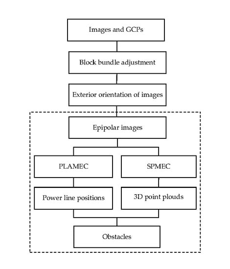
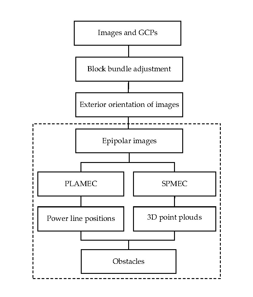
All of the objects in the power line corridor with a distance to the power line that is less than the safety distance are defined as obstacles [21]. As shown in Figure 1, to detect obstacles within the power line corridor, we first use UAV images and ground control points (GCPs) to obtain the exterior orientation of images (EOIs) via block bundle adjustment (BBA). Then, epipolar images are generated based on the relative orientation parameters of stereo images. Subsequently, PLAMEC is proposed to extract power line 3D vectors from stereo image pairs composed of corresponding images from different flight strips, and the semi patch matching based on epipolar constraints (SPMEC) is employed to extract dense point clouds from within the corridor for a 3D reconstruction of the ground objects, including canopies, buildings, and other ground attachments. Finally, obstacles are automatically identified and located by calculating the spatial distance between the power line and the ground point cloud extracted from the optical imagery.
The rest of this section is organized as follows. Section 2.1 describes the PLAMEC, which is the emphasis of this paper. Section 2.2 gives a brief description of the SPMEC, and Section 2.3 demonstrates the automatic detection of obstacles in a power line corridor.
2.1. Power Line Automatic Measurement Method Based on Epipolar Constraints
When inspecting the power line corridor for obstacles, the flight parameters mast be designed according the camera parameters mounted on a UAV. The flying height of UAVs should trade off the image ground sample distance (GSD) and the operational efficacy. The higher the above-ground height of the UAV, the higher the efficiency of the photography and the bigger the GSD value will become. The power line would be too thin to be imaged because of the small photographic scale. In general, the diameter of EHV power lines is about 4 cm. Therefore, in practice, we are inclined to design the flight height according to cm. The forward and side overlaps are also essential parameters, and we recommend that the forward and side overlaps both be set at 80%. A high forward overlap will increase the robustness of the automatic tie points measurement method in aerial triangulation (AT). A high side overlap will reduce the risk of the power line being outside of the overlap area of the stereo images. After determining the flight height, as well as the forward and side overlap, a UAV flies back and forth along the power line, collecting two strips as shown in Figure 2. Geo-referencing the images was conducted using a block bundle adjustment process and ground control points.
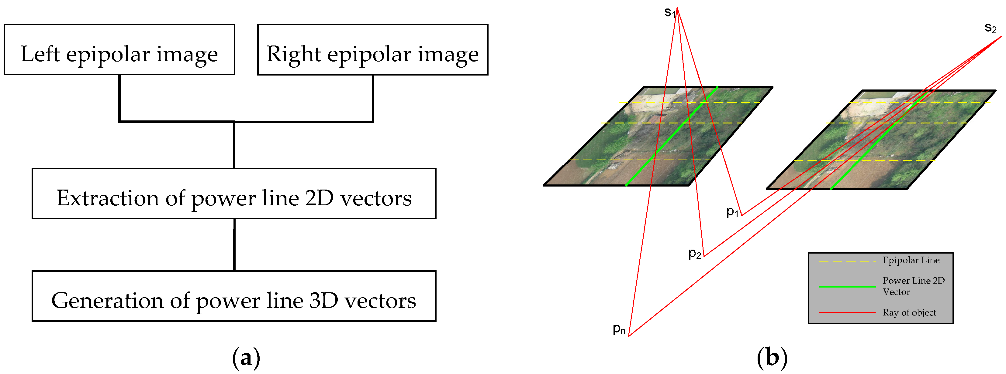
The diameter of a power line is small (about 4 cm); hence, the power line in an image is very thin and is usually approximately one to three pixels. The texture is homogenous, while the image background is composed of complex textures. It is difficult to use image-matching methods to find corresponding points along the power line. We propose PLAMEC to perform automatic power line measurements since the ground points in the stereo image pairs must be located along the corresponding epipolar lines. Figure 3 shows a flow chart of the proposed method.
As shown in Figure 3a, a pair of images from two adjacent strips are selected as the stereo image pairs, making the direction of the power line approximately perpendicular to that of the epipolar line. The epipolar images are generated based on the coplanarity condition, and the relative orientation parameters of the stereo image pair are calculated using the relative orientation algorithm [24]. Then, the power line automatic extraction algorithm is used to extract the 2D vectors of the power lines from the left and right epipolar images (as shown by the green solid lines in Figure 3b). Finally, in the direction of the y parallax of the epipolar image, pairs of corresponding epipolar lines are obtained at a certain interval (as shown by the yellow dashed lines in Figure 3b). The intersections of the epipolar and power line vectors in the left and right epipolar images are obtained, and the two intersections are a pair of corresponding points on the power line. The 3D coordinates can be obtained by forward intersection [24].
2.1.1. Automatic Extraction of Power Line 2D Vectors from Epipolar Images
The automatic extraction of power line 2D vectors requires epipolar images as input and 2D vectors of power lines as output. A flow chart for power line 2D vector extraction is shown in Figure 4.
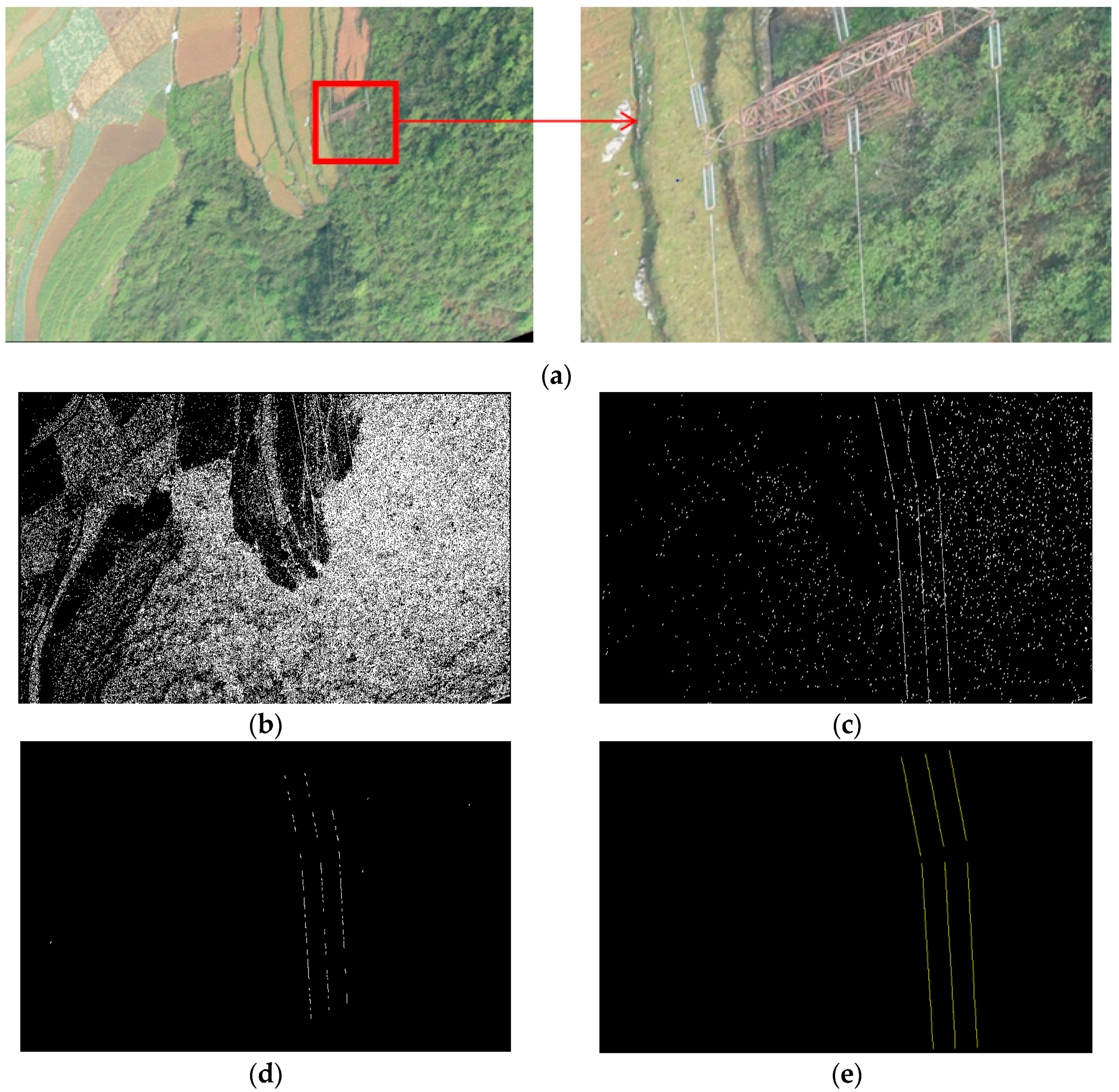
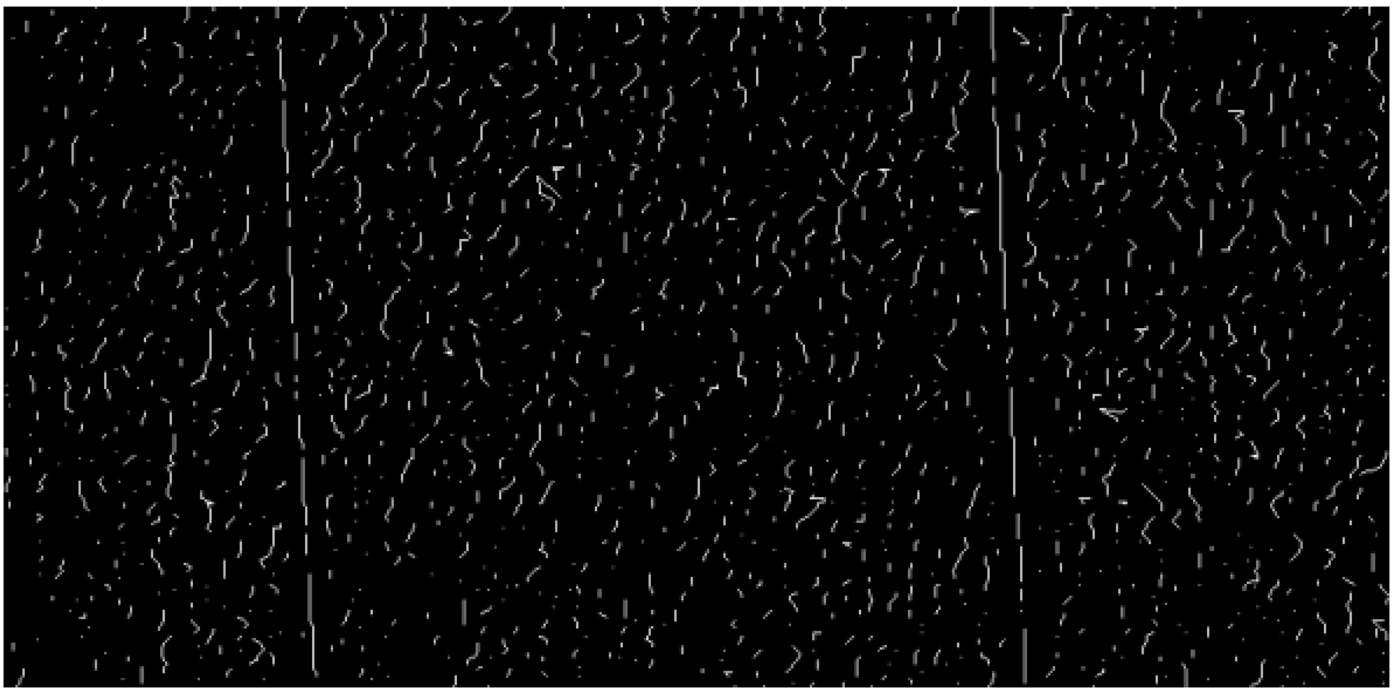
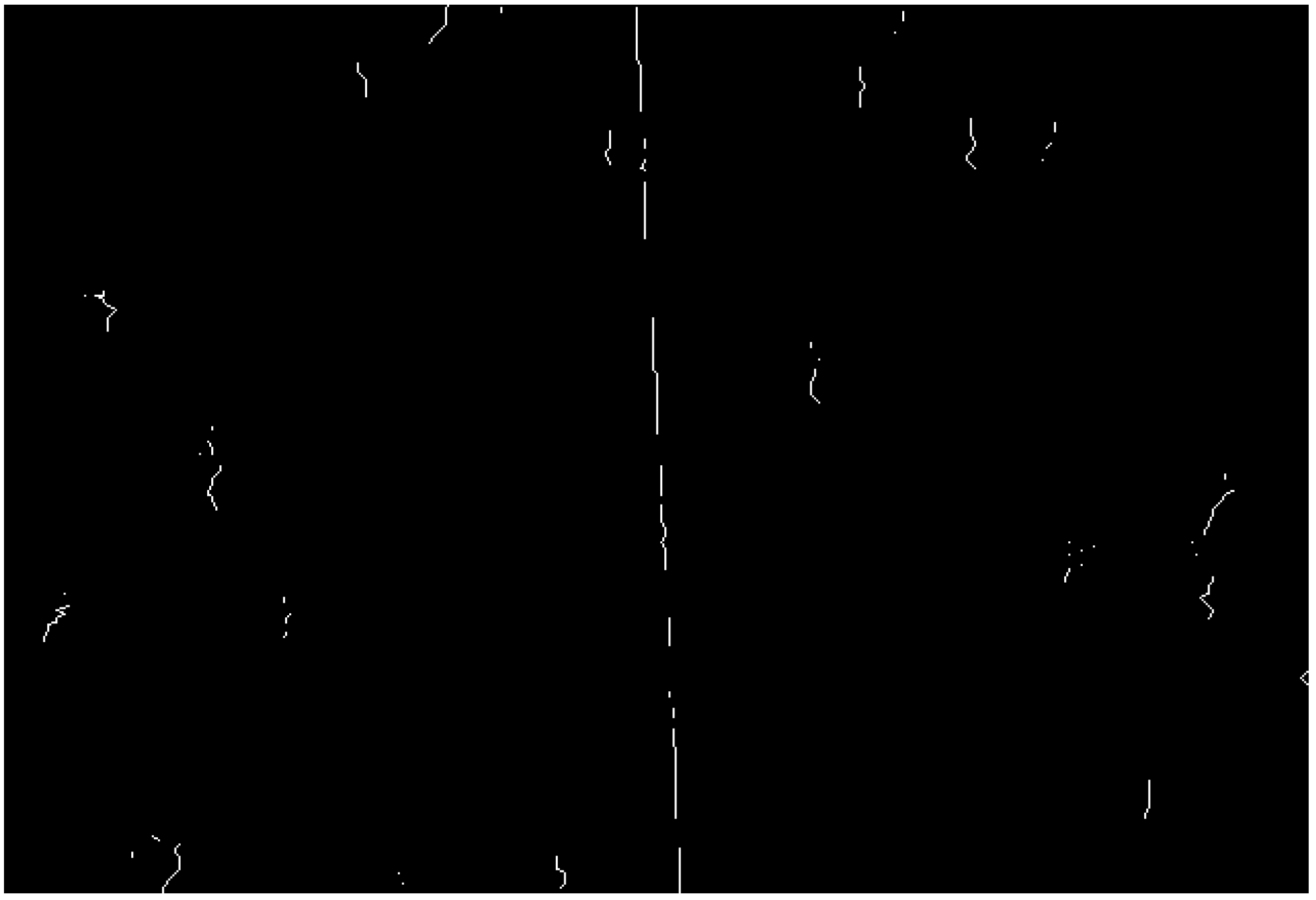
The process contains three steps: the detection of power line features using a gray ratio operator, the refinement of power line segments based on the same line conditions, and the extraction of power line vectors based on prior knowledge. This section describes these three steps. To better illustrate the proposed method, we visualize the results for each step: the left epipolar image of a stereo is shown in Figure 5a, the detected power line features are shown in Figure 5b, the refined power line segment results are shown in Figure 5c,d, and the extracted power line vectors are shown in Figure 5e.
Figure 5a shows the left epipolar image of a stereo. Figure 5b shows the results for line feature detection using a gray ratio operator. Due to the complexity of the background texture, there are many non-power line features in the feature extraction results. Based on an analysis of the difference between the power line features and non-power line features, a filter was designed to refine the feature detection results. The refinement result is shown in Figure 5c. After an initial refinement, the line segments belonging to the same power line are approximately collinear. Each line segment is extended, and a search is conducted for other collinear line segments, which is taken as a condition to judge whether the current segment is a power line segment, after which the power line extraction result is refined further as shown in Figure 5d. After being refined by two steps, the detection results are power line segments. Based on the prior knowledge of the power lines as shown in the image, the power line segments are linked, and a power line 2D vector result is output as shown in Figure 5e.
(1) Detection of Power Line Features Based on Gray Ratio Operators
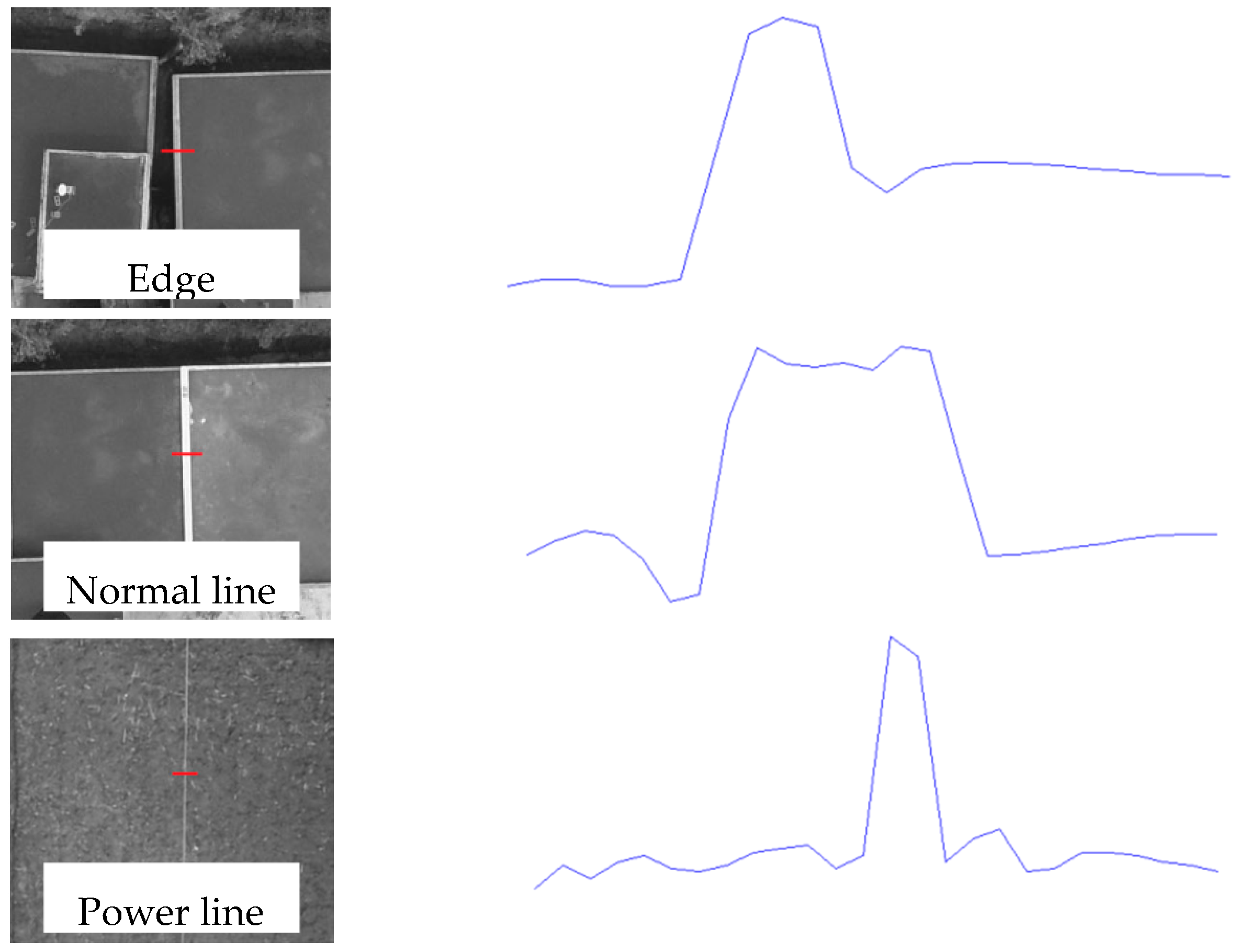
In the process of power line inspection, the direction of flight and flight height of a UAV are designed to ensure that the power line is clearly imaged. In general, the width of the power line in an image is one to three pixels. Power lines are distinguishable from other features, which can be used to design feature detection operators for power lines. Figure 6 shows three typical objects in a power line corridor that have strong edge responses with their corresponding gray value profiles.
From Figure 6, we can see that a power line is brighter (compared with the background, the metal material of power line usually has higher reflectance) and has a narrower peak in the gray profile compared to the edges of objects such as houses. The monotone minimum values on both sides of the wave peak are approximately the same because power lines have small diameters and have an approximately uniform texture on either side, which can be used to design feature detection operators for power lines, as shown in Figure 7.
In Figure 7, the blue curve shows the profile of the gray value of a row of pixels in an epipolar image. Three windows are arranged along the direction of the epipolar line, which are marked as , and (illustrated by the red squares shown in Figure 7). The size of each window is pixels, and the distance between the windows is pixels. The gray value sum of the three windows is calculated and marked as , after which the gray ratio is calculated for the area between the center window and the windows and . Windows and are shown as the windows on the left and right, respectively, according to Equation (1). If the ratio is greater than a threshold , the power line feature is detected, and the gray value of the central pixel in is marked as 255; otherwise, the gray value is marked as 0. In this way, the binary image of a power line feature detection result is generated as shown in Figure 5b.
In Equation (1), the numerator is the sum of the differences in the gray values between the center window and the windows on the left and right. Since a power line is brighter than the background, larger differences indicate a stronger contrast between the power line and the background. The denominator is the absolute value of the difference between the gray sum of the left window and the gray sum of the right window, as a power line has a small diameter with an approximately uniform texture on either side. To prevent the operator from division by 0, a value of 1 is added to the denominator. Given that the ground resolution of the UAV image is 4 to 5 cm and that the width of the power line is approximately one pure pixel with one mixed pixel of the power line and the ground on both the left side and the right side, the power line feature detection operator parameters are set as pixel, pixel, and . To ensure that the width in the binary image is a single pixel, a thinning algorithm based on mathematical morphology [25] is adopted to process the binary image of the power line features. During the power line feature detection process, only the ratio between the sum (the numerator) and the difference (the denominator) is calculated, which is compared with the threshold as a basis for judging the presence of a power line. Noise in the image is inevitable; there are a large number of small, discontinuous and randomly shaped non-power line segments in the detection results, as shown in Figure 8.
It can be seen from Figure 8 that, compared with power line features, non-power lines are shorter, more curved, and exhibit more space in their surroundings. The filter design starts by considering these characteristics and filtering out the micro scratch-like noises in the feature detection results without having a significant impact on the real power line features. First, a vector tracking algorithm [26] is used for the vectorization of the binary image of power line features, removing features that are shorter than seven pixels. A shape index (SI) of the remaining features is calculated according to Equation (2), thereby removing the curved features that are larger than 0.25 pixels.
In Equation (2), is the area of the polygon surrounded by the features, and is the perimeter of the polygon. Secondly, An HMT (hit or miss transform) based on mathematical morphology [25] is adopted to delete the isolated features.
(2) Power Line Segment Refinement Based on Equivalent Line Conditions
The power lines are actually consecutive line in the images; however, after the initial refinement of the detected line features, they are represented by discontinuous line segments because of background and sources of noise, as shown in Figure 5c. There are not only straight power line segments but also straight segments and curved segments of other linear objects, as shown in Figure 9.
A vector tracking algorithm [26] is used for the vectorization of the binary image, as shown in Figure 5c. For any line segment in the vector result, the extension line and the line segment intersecting the extension line for the first time are obtained. If the direction of the intersected line segment is consistent with the current line segment, then the current line segment is retained; otherwise, the current line segment is removed as noise. Non-power line sources of noise are significantly decreased, as a comparison between Figure 5c and Figure 5d shows. Consequently, equivalent line conditions of line segments effectively distinguish between power line and non-power line features.
(3) Power Line Vector Extraction Based on Prior Knowledge
In general, within an EHV transmission network, the distance between two towers is about 300 to 500 m. For a UAV image, the power lines run through the whole image, forming a set of parallel lines. Alternatively, there is one tower in the image, dividing the power lines into two sets of parallel lines. First, the power line segments are grouped according to the condition regarding whether they are parallel. For each set of parallel lines, a straight line is set parallel to them, and the distances between this straight line and the line segments are calculated. Subsequently, the power lines in the same set are divided into different groups by the differences in the distance. The line segments in the same group can be considered to belong to the same power line and are then connected end to end. Finally, the two ends of the power line are extended to make it the same length as the longest line in the same group of parallel lines.
2.1.2. Automatic Generation of Power Line 3D Vectors
As shown in Figure 3b, after extracting the 2D vectors of the power lines from the epipolar images, pairs of corresponding epipolar lines are obtained at certain intervals in the direction of the y parallax of the epipolar images. The intersections of the epipolar lines and corresponding power lines are calculated, and they form a pair of corresponding image points on the power line. The 3D coordinates of the corresponding points can be calculated using a forward intersection algorithm [24]. In this way, 2D vectors of power lines can be converted into 3D vectors.
There are two issues that should be addressed. One issue is the determination of the corresponding power line vectors extracted from the epipolar images. The other issue is the improvement of the positioning accuracy of the corresponding image points on the power line at the sub-pixel level.
(1) Selection of Corresponding Power Lines
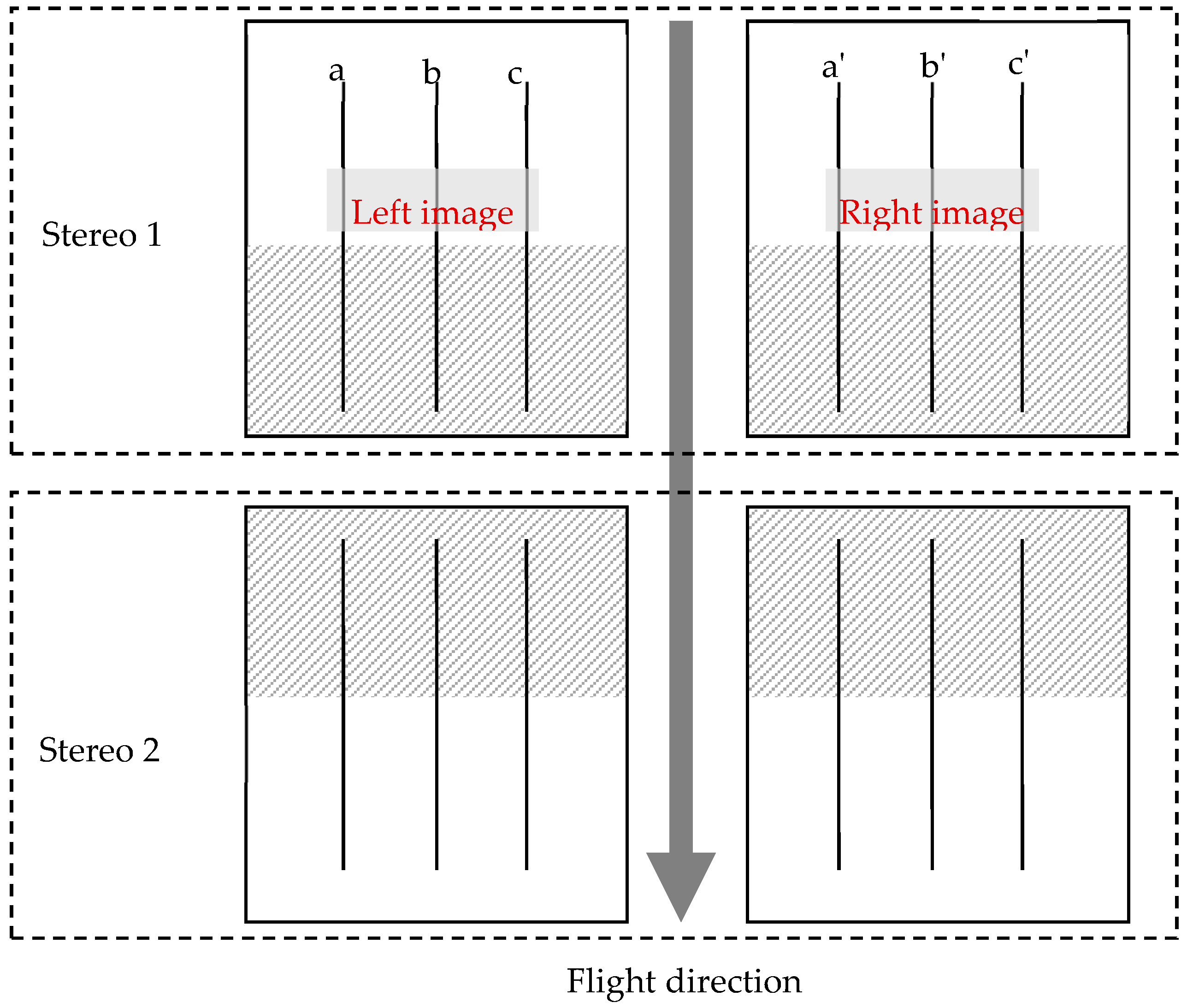
Automatically matching power line vectors is very difficult because the image textures surrounding the power lines are very similar. Thus, we applied manual work to match the power line vectors and consider them as the seeds. As shown in Figure 10, power lines a and a′ (Stereo 1) represent the manually selected corresponding power lines, and their 3D coordinates can be calculated by forward intersection. In the next stereo image pair (Stereo 2 in Figure 10), the corresponding power lines can be automatically determined by the re-projection of the 3D coordinates. The correspondence of the rest of the power lines can be conducted in the same manner.
(2) Sub-Pixel Level Positioning of the Corresponding Points along the Power Lines
To ensure that the accuracy during the automatic measurement of power lines is consistent with that of manual measurements, the accuracy of the intersection positioning must be determined at the sub-pixel level. The positioning accuracy of the 2D power line vectors in the epipolar images achieved by the method discussed in Section 2.1.1 is expressed in pixels, and thus, the positioning accuracy of the intersections between the epipolar and power lines is only at the pixel level. During manual stereo measurement, the positioning accuracy of the stereo marks in both the left and right epipolar images is approximately 0.5 pixels. To achieve sub-pixel accuracy, we calculate the intersection between the epipolar line and the power line. The gray ratio coefficient between the intersection point and the adjacent pixels on the left and right sides are calculated according to Equation (1). We adopt a parabolic fitting algorithm [24] to acquire the coordinates for the maximum value of the coefficients, which are used as the true intersection between the epipolar line and the power line 2D vector.
2.2. Power Line Corridor 3D Reconstruction Using the SPMEC
Modern 3D reconstruction algorithms include patch base multi-view system (PMVS) [27], multi-photo geometry constrains (MPGC) [28] and semi-global matching (SGM) [29]. For an efficient matching algorithm, we applied the SPMEC, which was proposed in reference [21]. The principle of the SPMEC is as follows: first, an initial parallax mesh is constructed using tie points; second, the match window slides along the epipolar line within a certain search window guided by the initial parallax; finally, a tentative match is determined by applying a similarity measure for the shape of the correlation coefficient curve within a certain search window, and the 3D reconstruction process is completed.
2.3. Automatic Detection of Obstacles within a Power Line Corridor
After extracting the power line and the 3D point clouds of the power line corridor, we divide the power line into n segments with δ as the step distance. When δ is small enough, each segment can be regarded as a straight line. If there is a point within the 3D point clouds at a distance from the straight line that is less than the safety distance, an obstacle can be detected, and the exact position of the obstacle is determined.
3. Results and Discussion
3.1. Basic Conditions of the Experimental Data
A typical working environment of a power line corridor inspection area located in Guizhou Province, southwestern China, is selected to test the proposed method. The province has a subtropical humid monsoon climate, abundant rainfall, dense vegetation cover, and undulating terrain. There are approximately 19,537 km of power lines with a voltage degree above 110 kV in Guizhou Province [30]. We select a section of a 220 kV power line that is approximately 3.9 km in length. The elevation difference along the power line corridor is approximately 200 m. There are nine towers within the selected power line corridor (Numbered: T108-T116). Each tower has three separated power lines, and thus, the total length of the power lines is 11.7 km (). The same fixed-wing UAV found in reference [21], with a Nikon D810 camera (focal length: 51.42 mm, complementary metal oxide semiconductor (CMOS) sensor, 35.9 mm × 24.0 mm, 7360 × 4912 pixels, pixel size: 4.88 ) is adopted for the photography of the power line corridor. The camera interior parameters were calibrated before commencing aerial photography. The images were shot at a fixed distance. The forward and side overlaps were both 80%. The relative height of the UAV to the ground is approximately 400 m. The height of each power line tower is approximately 25 m. The GSD is approximately 3.8 cm. Two strips were flown, and 178 valid photos were acquired. The strip arrangement and topography are shown in Figure 11. The edges of the image are sharp and without obvious blurring, and the contrast is moderate, without over-exposure or under-exposure; therefore, they meet the requirements of power line inspection. All of the images are geo-referenced using an aerial photogrammetric triangulation process.
The PLAMEC algorithm was verified by experiments, including the 2D power line vector extraction capability and extraction accuracy. The accuracy of the automatic 3D reconstruction of power lines was evaluated by comparing the automatic generation of 3D power line vectors and the results of manual power line measurements. The 3D reconstruction of the ground of the power line corridor was achieved using the SPMEC. Taking 6.5 m as the threshold, the obstacles in the corridor were automatically detected. An obstacle distribution table was output, and the values were checked through a field investigation to verify the practicability of the proposed method.
3.2. Analysis of the Block Bundle Adjustment
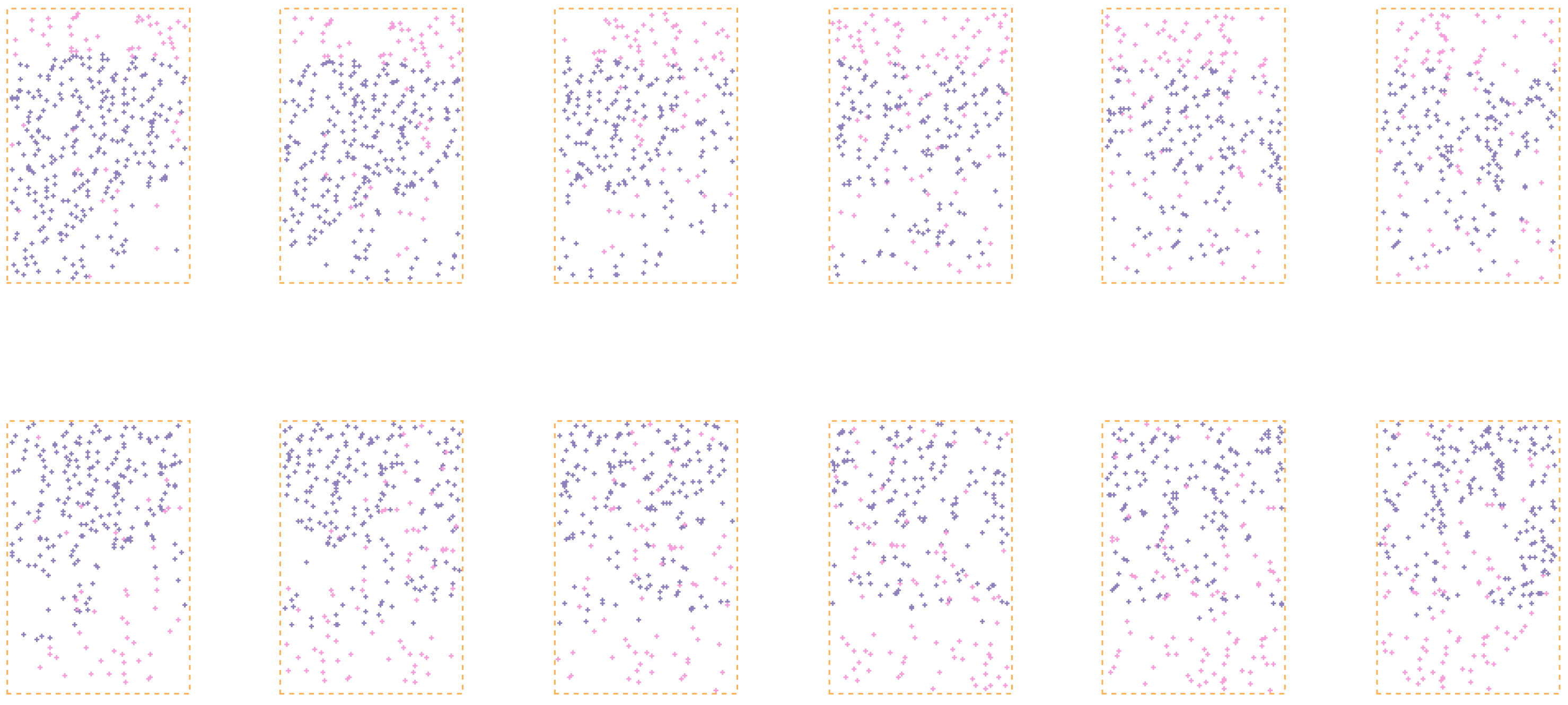
We employed the block bundle adjustment (BBA) software, PATB [31] to obtain EOIs. Tie points were initially matched using the scale-invariant feature transform (SIFT) [32] descriptor and refined by least square matching [33]. Part of the tie points are shown in Figure 12.
From Figure 12, we can see that, for each image, there are 200~300 evenly distributed tie points. We surveyed the coordinates of 15 ground points along the power line corridor and used 11 points as GCPs in BBA and four of them as check points. The distribution of these ground points is shown in Figure 13.
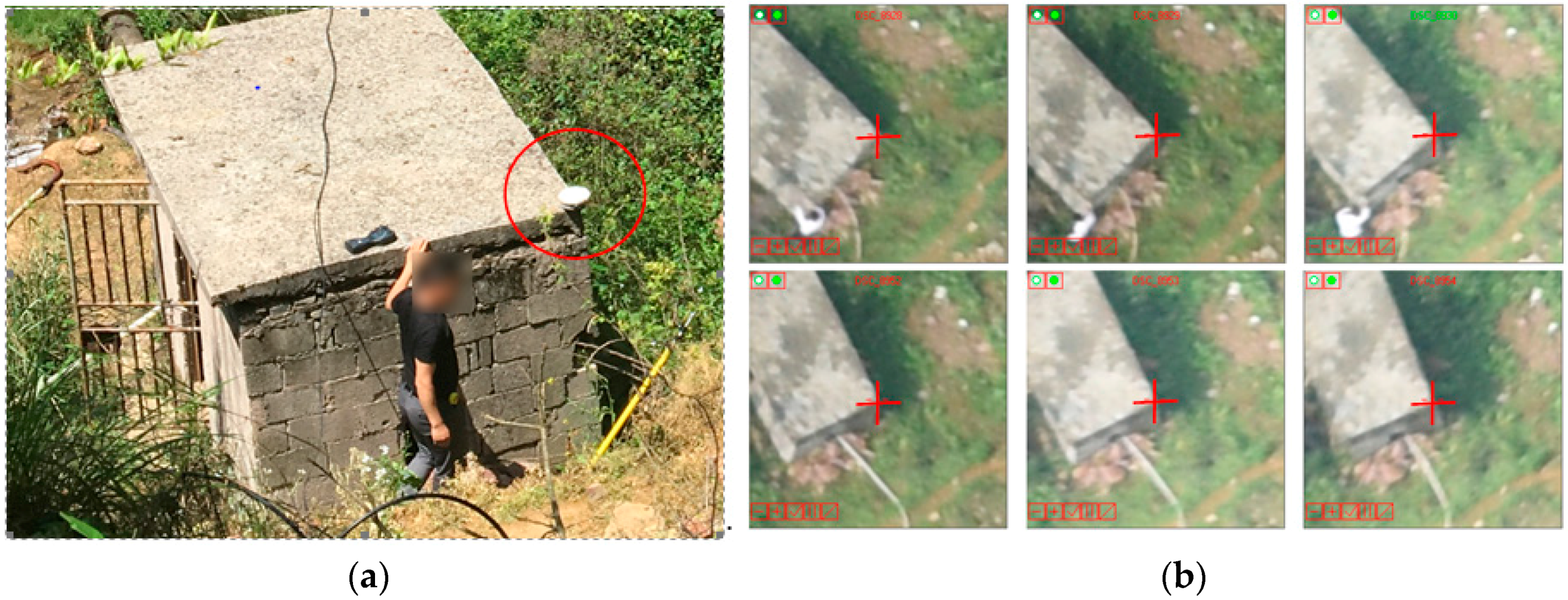
All GCPs and check points are located on easily identifiable corners of ground objects. The coordinates were surveyed using a global navigation satellite system (GNSS) real-time kinematic (RTK) and calculated using the continuously operating reference stations (CORS) system in the CGCS-2000 coordinate system. The re-projected image coordinates of the GCPs were measured manually. The location and image measurement of GCP No. 9012 are shown in Figure 14.
Before applying BBA, we used the precise point position (PPP) algorithm [34] to calculate the coordinates of the antenna phasing center associated with the onboard GNSS receiver, for each image at the instant of exposure. Subsequently we input all tie points, GCP coordinates, and antenna phasing center coordinates to the PATB software. Since image distortion was corrected, we did not use camera self-calibration during PATB analysis. After BBA, we used adjacent image pairs from the same strip as stereo image pairs and measured all check points using stereo-measurement software. The difference between the field surveyed coordinates and software measured coordinates are shown in Table 1.
From Table 1, we can see that the manually-measured coordinates of check points using stereo-measure software are quite consistent with the coordinates surveyed in the field. The maximum differences of the easting, northing, and elevation of the check points are 0.125 m, 0.166 m and −0.385 m, and the root mean square (RMS) errors are 0.073 m, 0.081 m and 0.233 m, respectively. Since the coordinates of check points were measured using a stereo image pair within a strip, the accuracy thus can be considered representative of the accuracy of SPMEC.
In this same way, we used adjacent images pairs from inter-strip as stereo image pairs and measured all check points using the stereo-measure software. The difference between the field surveyed coordinates and software measured coordinates are shown in Table 2.
As shown in Table 2, the coordinates of check points measured from inter-strip stereo image pair were also quite consistent with the coordinates measured in the field. The maximum differences of the easting, northing and elevation of the check points are −0.156 m, 0.122 m and 0.305 m, and the RMS errors are 0.075 m, 0.085 m and 0.205 m, respectively. Since the coordinates of check points was measured using inter-strip stereo image pair, the accuracy thus can be used as the accuracy of PLAMEC.
From Table 1 and Table 2, we can see that the planar coordinates are almost the same using either the stereo image pair from in-strip or inter-strip. When the overlap of in-strip and inter-strip stereo images are both 80% and the shape of the onboard sensor is a rectangle, then the base line of the inter-strip image pair is slightly longer than an in-strip image pair. Thus, the elevation accuracy from the inter-strip stereo pair was slightly higher than the accuracy of the in-strip stereo pair.
3.3. Analysis of the Results of Automatic Power Line Measurements
To verify the feasibility of the PLAMEC technique proposed in Section 2.1, the power lines in the experimental area were automatically measured to have a total length of 10.9 km. In the experimental area we chose, there were three power lines on the towers, reaching a total length of 11.7 km. Thus, the success rate for automatic extraction of power line was 93.2%.
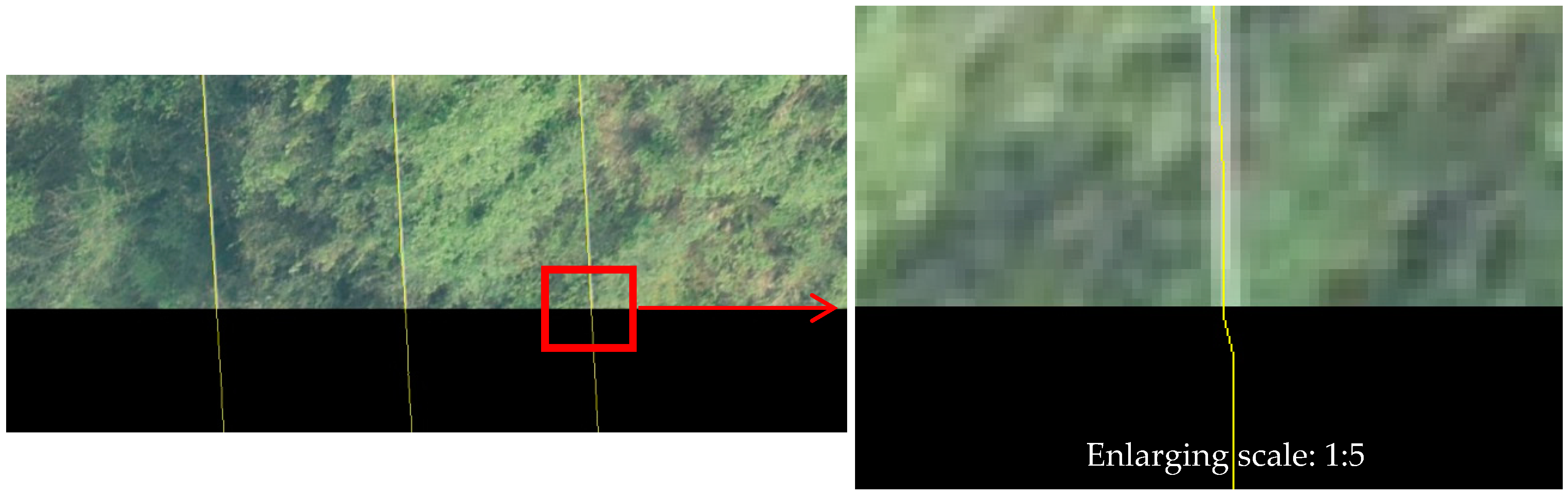
To further verify the measuring accuracy of power lines using the PLAMEC, we registered the epipolar images with the extracted power line 2D vectors, as shown in Figure 15, and evaluated the accuracy by visual comparison.
As shown in Figure 15, power line 2D vectors can be registered accurately with the power lines in the epipolar image. We manually checked 89 (178/2 = 89) stereo image pairs and found that the estimated registration error is approximately one pixel. The registration results are consistent with the location accuracy of the proposed power line feature detector.
According to the method introduced in Section 2.1.2, after the generation of 3D vectors from the power line 2D vectors, we compared the automatic measurement and stereoscopic manual measurements on the stereo image pairs, which were performed on photogrammetric software MapMatrix [35]. Fourteen of the checking points were evenly extracted to compare the elevation differences between the automatic and the manual measurements. The results are shown in Table 3.
It can be seen from Table 3 that the RMS error of the elevation differences between the automatic measurement results and the manual measurement results is 0.148 m. The maximum error was 0.243 m, which shows that the accuracy of the automatic measurement is consistent with the manual measurement method. We infer that our proposed approach can replace the manual measurement of power lines during the inspection of power line corridors.
3.4. Detection of Obstacles within the Power Line Corridor
We use 6.5 m as the safe distance threshold between the power line and ground objects. As a result, we detect eight obstacles, as shown in Figure 16.
In Figure 16, the ground 3D point clouds were extracted using the SPMEC, while the blue, orange, and white wires were measured using the PLAMEC. The red points are obstacles. The towers with existing 3D models were included in the scene to make it more intuitive. Taking the power line corridor between T109 and T110 in the experimental area as an example, Figure 17 shows the profile analysis of the power line and the ground.
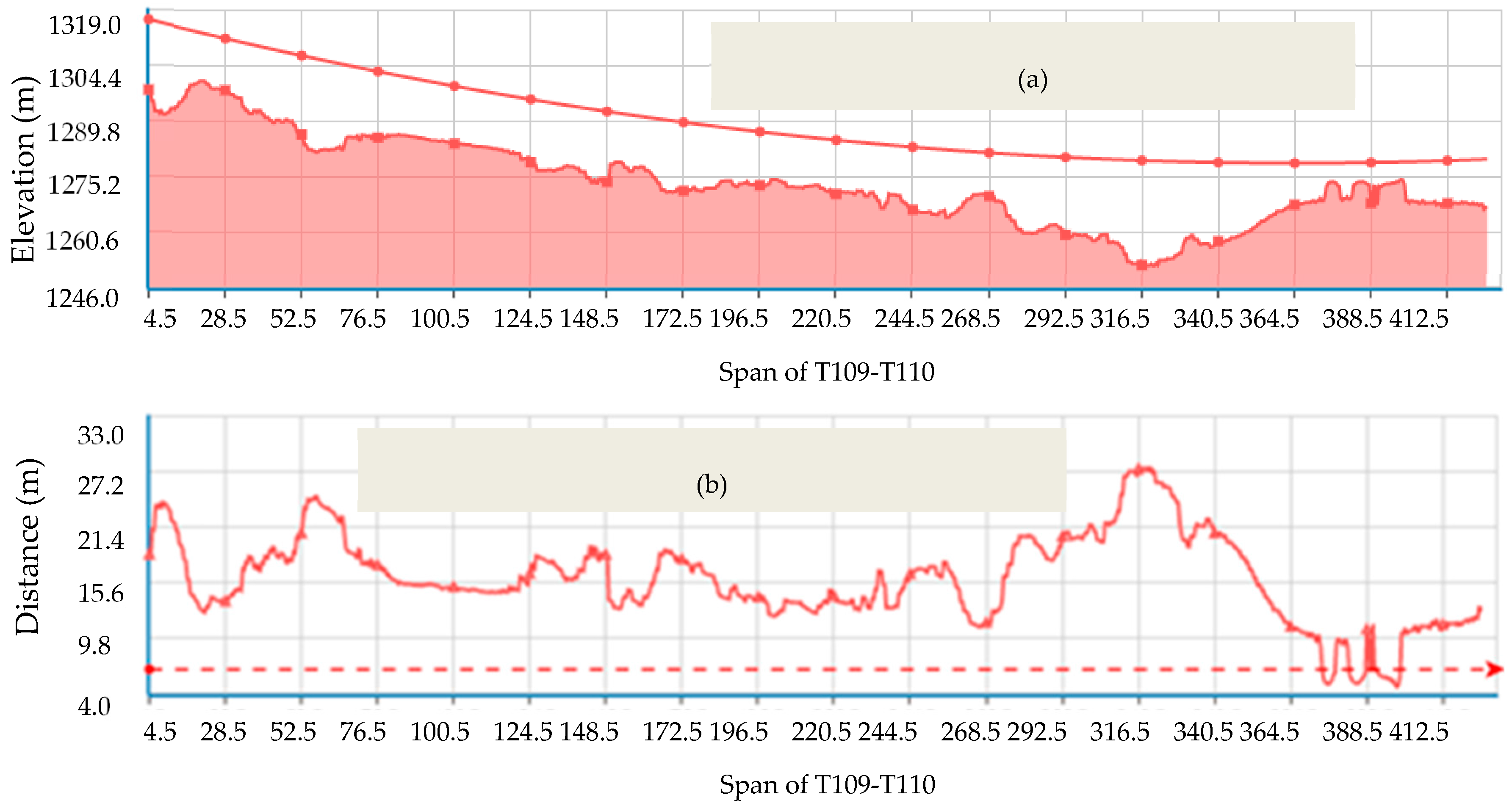
Figure 17a represents the profile of the power line corridor, where the horizontal axis shows the distance to T109 and the vertical axis shows the elevation. Figure 17b represents the distance between the power line and the ground, where the horizontal axis shows the distance to T109 and the vertical axis shows the distance. It can be seen from Figure 17b that, when the safe distance between the power line and the ground is set to 6.5 m, an obstacle that is 388.5 m away from T109 can be detected.
The positions of the eight obstacles and the distances between them and the power line are listed in Table 4. To verify the reliability of the obstacle detection results, a field investigation was conducted. The distances between the obstacles and the power line were measured using TruPulse 200, a laser range finder produced by Laser Technology, Inc. [36]. These results are also listed in Table 4.
In Table 4, the first column is the identifications of the towers, the second column represents the distances between the obstacles and the first tower, and the third column gives the results of the distances between the obstacles and the power line obtained using the proposed method and the field measurements. The differences between the distances obtained using the two methods are also given in the fourth column. As shown in Table 4, the distances between the obstacles and the power lines obtained by the proposed method conform to the field measurement results. The RMS error of the differences between the distances was 0.319 m, and the maximum error was 0.420 m. While verifying the distance between obstacles and power lines, we use a laser range finder instead of a total station, because a laser range finder is easier to operate. Another reason for using a laser range finder is that, even when using a total station, it is very hard to determine the location of a point on a power line with a minimum distance to the canopy. Conversely, a canopy is a large object and therefore it is a difficult task to determine the location of a point on a canopy when the minimum distance to the power line depends on the viewpoint of an operator. Thus, we followed the traditional specifications, and used a laser range finder to measure multiple times to confirm the detected obstacles in our proposed method. The accuracy of the laser range finder used in the experiments is about 0.3 m [37], which is consistent with the proposed method. Thus, it cannot be used as ground truth to check the accuracy of the proposed obstacle detection method. Although the method is not designed to assess the accuracy of the measured distance between obstacles and power lines, the distance measured by this method is consistent with the traditional methods, and meets the requirements (better than 2 m) for the inspection of obstacles within power line corridors. To further verify whether there are undetected obstacles in the experimental power line corridors, we manually checked all the stereos in the stereo measurement system, and found that no obstacle was missed in the automatic detection, which meet the needs of power line inspection.
4. Conclusions
In this paper, we proposed an automatic inspection method for power lines using UAV images. We focused on solving three problems: the automatic measurement of power lines, the automatic 3D reconstruction of the ground along the power line corridor, and the automatic recognition of obstacles. We proposed the PLAMEC for automatic measurements of power lines, based on the principle that the intersection point of the epipolar line and the corresponding power line must be the corresponding image point on the power line. The SPMEC algorithm was adopted for a 3D reconstruction of the ground along the power line corridor, and the obstacles could be detected automatically by calculating the distance between the 3D vectors of the power lines and the ground point clouds. The results showed that the success rate of the automatic measurement of power lines was 93.2%, and the accuracy was consistent with those of manual measurements, indicating that it can replace the manual measurement of 3D coordinates of power lines. The height RMS error of the point cloud was 0.233 m and the RMS error of the power line was 0.205 m. During the test, when the distance threshold was set to 6.5 m, eight obstacles were found. The distances between the obstacles and the power lines conformed approximately to the field-measured results; the measured distance difference between the two methods was better than ±0.5 m. Due to the limitations inherent to actual application scenarios on the ground, at this point, we cannot acquire the true distance between the obstacles and power lines to assess the true distance measurement accuracy, which will be addressed in our future studies.
Acknowledgments
This work was supported by the National Natural Science Foundation of China (Grants. 41371432, 41401522) and the National Key Developing Program for Basic Sciences of China (Grant No. 2012CB719902).
Author Contributions
Yong Zhang developed the algorithm, conducted the primary data analysis, and crafted the manuscript. Xiuxiao Yuan advised on the data analysis provided remote sensing experience and significantly edited the manuscript. Wenzhuo Li and Shiyu Chen carried out the experiments and revised the manuscript.
Conflicts of Interest
The authors declare no conflict of interest.
References
- Miralles, F.; Pouliot, N.; Montambault, S. State-of-the-art review of computer vision for the management of power transmission lines. In Proceedings of the IEEE International Conference on Applied Robotics for the Power Industry (CARPI), Foz do Iguassu, Brazil, 14–16 October 2014. [Google Scholar]
- Ahmad, J.; Malik, A.S.; Abdullah, M.F.; Kamel, N.; Xia, L. A novel method for vegetation encroachment monitoring of transmission lines using a single 2D camera. Pattern Anal. Appl. 2015, 18, 419–440. [Google Scholar] [CrossRef]
- Matikainen, L.; Lehtomäki, M.; Ahokas, E.; Hyyppä, J.; Karjalainen, M.; Jaakkola, A.; Kukko, A.; Heinonen, T. Remote sensing methods for power line corridor surveys. ISPRS J. Photogramm. Remote Sens. 2016, 119, 10–31. [Google Scholar] [CrossRef]
- Zhang, J.X.; Huang, G.M.; Liu, J.P. SAR remote sensing monitoring of the Yushu earthquake disaster situation and the information service system. J. Remote Sens. 2010, 14, 1–046. [Google Scholar]
- Eriksson, L.E.B.; Fransson, J.E.S.; Soja, M.J.; Santoro, M. Backscatter signatures of wind-thrown forest in satellite SAR images. In Proceedings of the IEEE International Geoscience and Remote Sensing Symposium (IGARSS), Munich, Germany, 22–27 July 2012. [Google Scholar]
- Kobayashi, Y.; Karady, G.G.; Heydt, G.T.; Olsen, R.G. The utilization of satellite images to identify trees endangering transmission lines. IEEE Trans. Power Deliv. 2009, 24, 1703–1709. [Google Scholar] [CrossRef]
- Mills, S.J.; Castro, M.P.G.; Li, Z.; Cai, J.; Hayward, R.; Mejias, L.; Walker, R.A. Evaluation of aerial remote sensing techniques for vegetation management in power-line corridors. IEEE Trans. Geosci. Remote Sens. 2010, 48, 3379–3390. [Google Scholar] [CrossRef] [Green Version]
- Sun, C.; Jones, R.; Talbot, H.; Wu, X.; Cheong, K.; Beare, R.; Buckley, M.; Berman, M. Measuring the distance of vegetation from powerlines using stereo vision. ISPRS J. Photogramm. Remote Sens. 2006, 60, 269–283. [Google Scholar] [CrossRef]
- Tabor, A.; Ottesen, B.S. Advances in applications for aerial infrared thermography. Proc. SPIE 2006, 156, 3642–3643. [Google Scholar]
- Guo, B.; Li, Q.; Huang, X.; Wang, C. An improved method for power-line reconstruction from point cloud data. Remote Sens. 2016, 8, 36. [Google Scholar] [CrossRef]
- Zhu, L.; Hyyppä, J. Fully-automated power line extraction from airborne laser scanning point clouds in forest areas. Remote Sens. 2014, 6, 11267–11282. [Google Scholar] [CrossRef]
- Mclaughlin, R.A. Extracting transmission lines from airborne LIDAR data. IEEE Geosci. Remote Sens. Lett. 2006, 3, 222–226. [Google Scholar] [CrossRef]
- Ax, M.; Thamke, S.; Kuhnert, L.; Kuhnert, K.-D. UAV based laser measurement for vegetation control at high-voltage transmission lines. Adv. Mater. Res. 2012, 614–615, 1147–1152. [Google Scholar] [CrossRef]
- RIEGEL. Available online: http://www.riegl.com/products/unmanned%E2%80%90scanning/ (accessed on 20 July 2017).
- Velodyne LiDAR. Available online: http://velodynelidar.com/products.html (accessed on 20 July 2017).
- Toth, J.; Gilpin-Jackson, A. Smart view for a smart grid—Unmanned Aerial Vehicles for transmission lines. In Proceedings of the 2010 1st International Conference on Applied Robotics for the Power Industry (CARPI), Montreal, QC, Canada, 5–7 October 2010. [Google Scholar]
- Cai, J.; Walker, R. Height estimation from monocular image sequences using dynamic programming with explicit occlusions. IET Comput. Vis. 2010, 4, 149–161. [Google Scholar] [CrossRef]
- Jóźków, G.; Vander Jagt, B.; Toth, C. Experiments with UAS imagery for automatic modeling of power line 3D geometry. Int. Arch. Photogramm. Remote Sens. Spat. Inf. Sci. 2015, XL-1/W4, 403–409. [Google Scholar]
- Jiang, S.; Jiang, W.; Huang, W.; Yang, L. UAV-based oblique photogrammetry for outdoor data acquisition and offsite visual inspection of transmission line. Remote Sens. 2017, 9, 278. [Google Scholar] [CrossRef]
- Deng, C.; Wang, S.; Huang, Z.; Tan, Z.; Liu, J. Unmanned Aerial Vehicles for power line inspection: A cooperative way in platforms and communications. J. Commun. 2014, 9, 687–692. [Google Scholar] [CrossRef]
- Zhang, Y.; Yuan, X.; Fang, Y.; Chen, S. UAV low altitude photogrammetry for power line inspection. ISPRS Int. J. Geo-Inf. 2017, 6, 14. [Google Scholar] [CrossRef]
- Ramesh, K.N.; Murthy, A.S.; Senthilnath, J.; Omkar, S.N. Automatic detection of powerlines in UAV remote sensed images. In Proceedings of the 2015 International Conference on Condition Assessment Techniques in Electrical Systems (CATCON), Bangalore, India, 10–12 December 2015. [Google Scholar]
- Yan, G.; Li, C.; Zhou, G.; Zhang, W.; Li, X. Automatic extraction of power lines from aerial images. IEEE Geosci. Remote Sens. Lett. 2007, 4, 387–391. [Google Scholar] [CrossRef]
- Zhang, Z.X.; Zhang, J.Q. Digital Photogrammetry; Wuhan University Press: Wuhan, China, 1997. [Google Scholar]
- Serra, J. Image Analysis and Mathematical Morphology; Academic Press: Orlando, FL, USA, 1982. [Google Scholar]
- Ren, M.; Yang, J.; Sun, H. Tracing boundary contours in a binary image. Image Vis. Comput. 2002, 20, 125–131. [Google Scholar] [CrossRef]
- Furukawa, Y.; Ponce, J. Accurate, dense, and robust multi-view stereopsis. IEEE Trans. Pattern Anal. Mach. Intell. 2010, 32, 1362–1376. [Google Scholar] [CrossRef] [PubMed]
- Zhang, L.; Gruen, A. Multi-image matching for DSM generation from IKONOS imagery. ISPRS J. Photogramm. Remote Sens. 2006, 60, 195–211. [Google Scholar] [CrossRef]
- Hirschmuller, H. Accurate and efficient stereo processing by semi-global matching and mutual information. In Proceedings of the 2005 IEEE Computer Society Conference on Computer Vision and Pattern Recognition (CVPR), San Diego, CA, USA, 20–26 June 2005. [Google Scholar]
- China Southern Power Grid. Available online: http://www.gz.csg.cn/web/news/43.html (accessed on 6 April 2017).
- k2-Photogrammetry. Available online: http://www.k2-photogrammetry.de/products/patb.html (accessed on 15 June 2017).
- Lowe, D.G. Distincitive image features from scale-invariant keypoints. Int. J. Comput. Vis. 2004, 60, 91–110. [Google Scholar] [CrossRef]
- Gruen, A. Adaptive least squares correlation: A powerful image matching technique. S. Afr. J. Photogramm. Remote Sens. Cartogr. 1985, 14, 175–187. [Google Scholar]
- Teunissen, P.J.G.; Khodabandeh, A. Review and principles of PPP-RTK methods. J. Géod. 2015, 89, 217–240. [Google Scholar] [CrossRef]
- Visiontek Inc. Available online: http://en.visiontek.com.cn/pp1/newsCategoryId=37.html (accessed on 18 July 2017).
- Laser Technology Inc. Available online: http://www.lasertech.com (accessed on 6 June 2017).
- Laser Technology Inc. Available online: http://www.lasertech.com/ftp/techdocs/TruPulse_Height_Performance.pdf (accessed on 20 July 2017).
Figure 1.
The workflow for the automatic detection of obstacles in power line corridors.
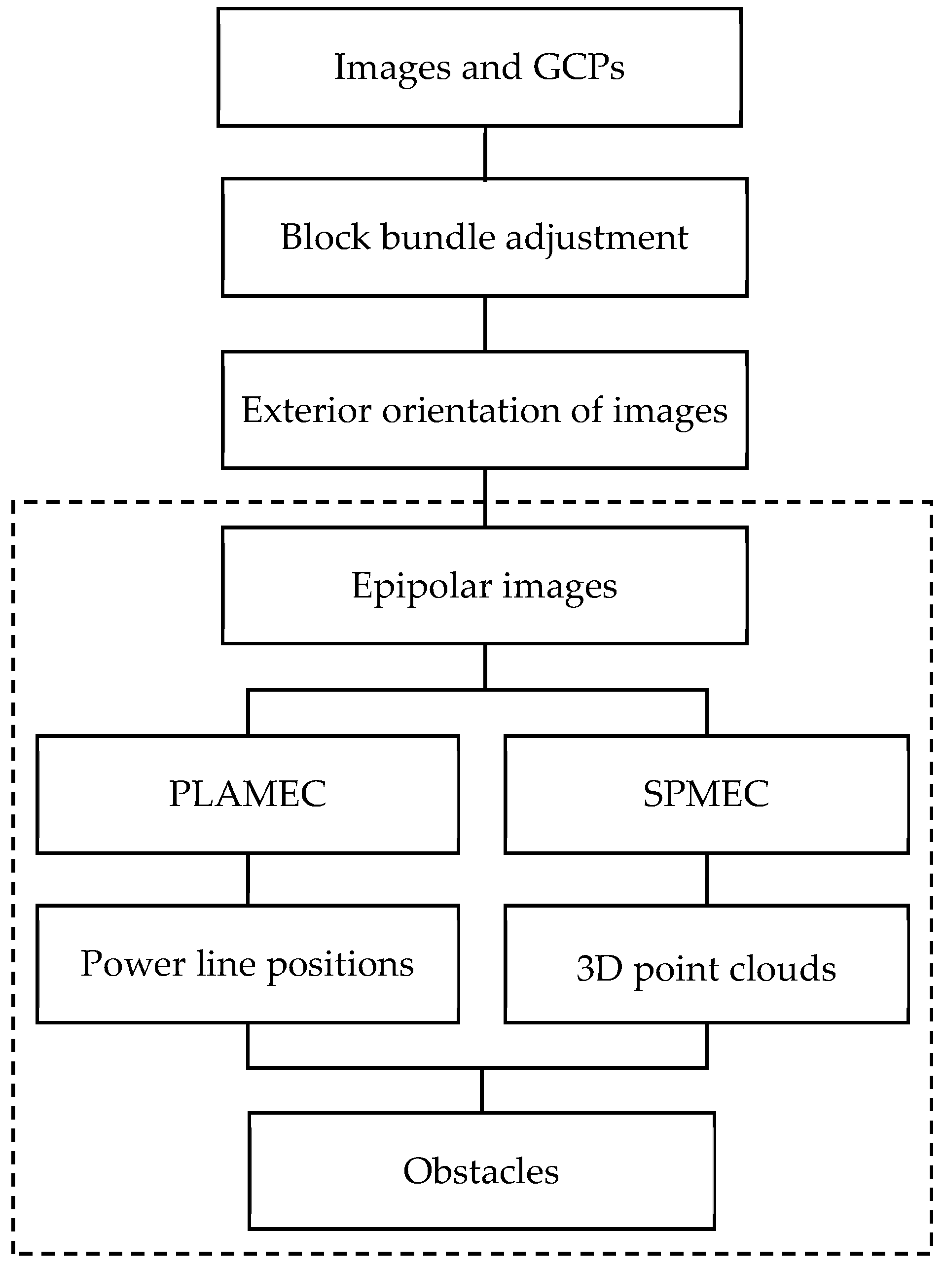
Figure 2.
Schematic diagram of the strip arrangement. The green dots represent camera centers, and the gray rectangles below the green dots are the captured images in world coordinates. The small dots at the bottom are the projected ground points where the color represents different elevations indicated by the legend on the right in the figure.
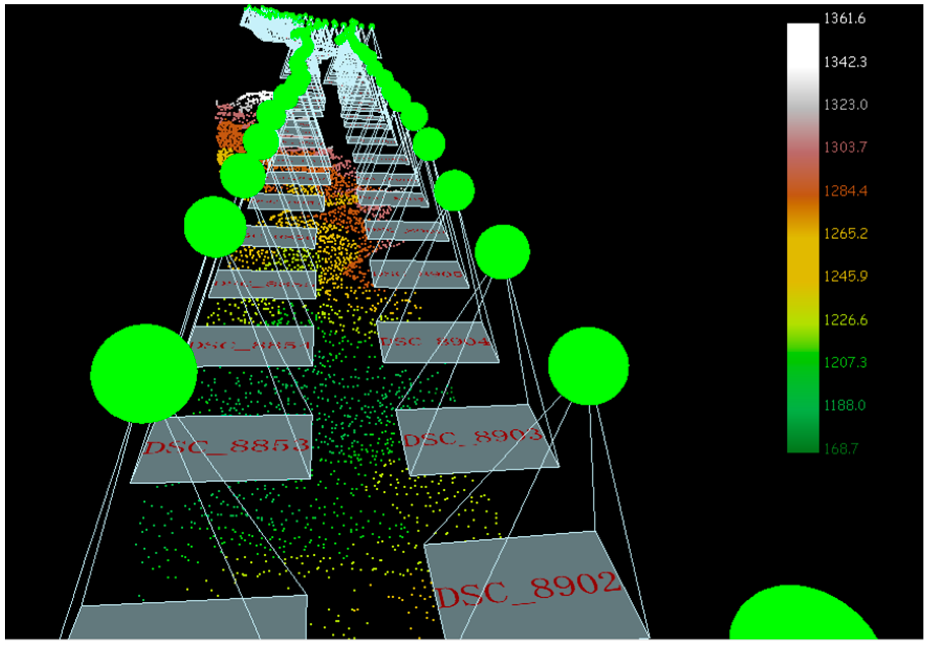
Figure 3.
Schematic diagrams of the automatic power line measurement method. (a) Flow chart for the power line automatic measurement method based on epipolar constraints (PLAMEC); (b) Visualization of the PLAMEC.
Figure 3.
Schematic diagrams of the automatic power line measurement method. (a) Flow chart for the power line automatic measurement method based on epipolar constraints (PLAMEC); (b) Visualization of the PLAMEC.

Figure 4.
Flow chart of power line 2D vector extraction.
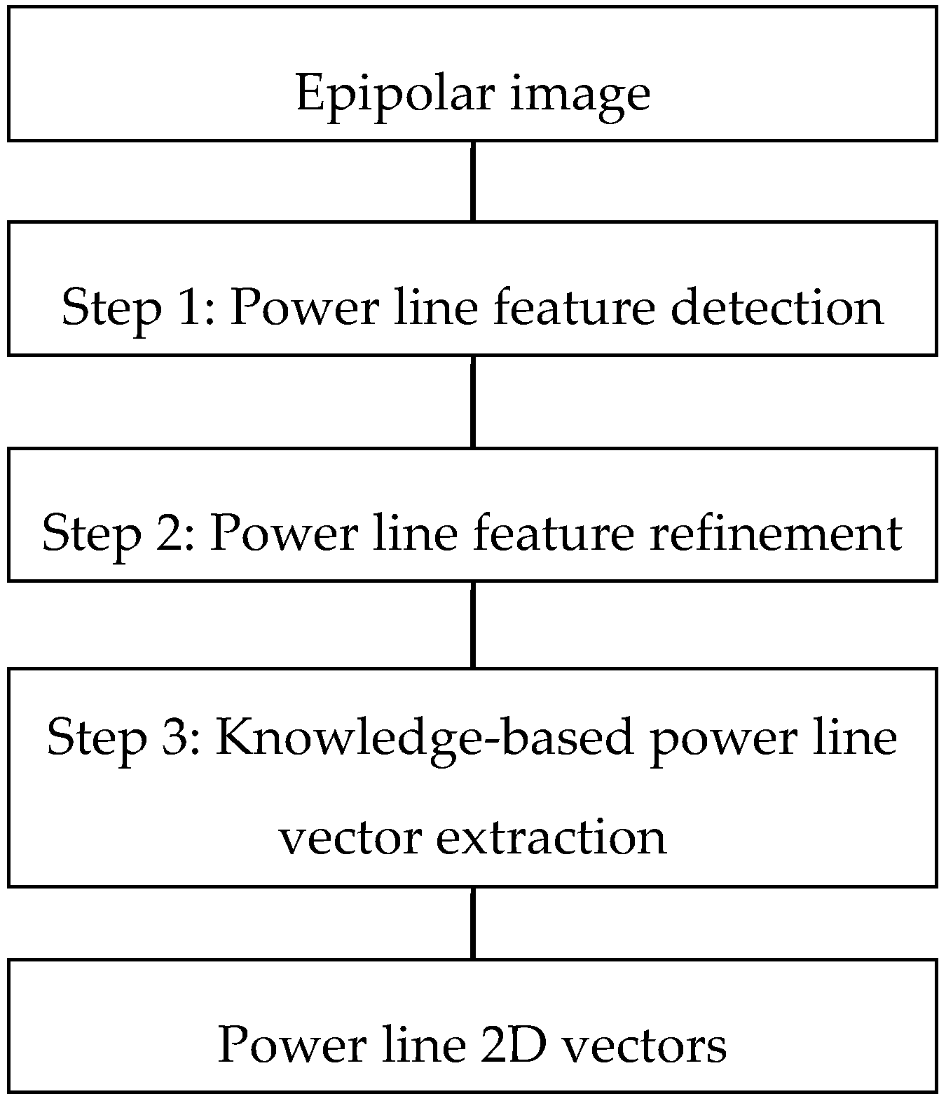
Figure 5.
Visualization of power line extraction. (a) Left epipolar image of a stereo; (b) Result of power line feature detection using a gray ratio operator; (c) Result of the refinement of power line features using mathematical morphology; (d) Result of the refinement of power line features using the equivalent line condition; (e) Result of power line 2D vector extraction by prior knowledge.

Figure 6.
Typical features of power lines that differ from other objects. Blue curves are the gray value profiles of the red segments in the images on the left.
Figure 6.
Typical features of power lines that differ from other objects. Blue curves are the gray value profiles of the red segments in the images on the left.

Figure 7.
Schematic diagram of a power line feature extraction operator.

Figure 8.
Partially enlarged image of the power line feature extraction result.

Figure 9.
Partially enlarged image of the results of the first refinement of power line features.

Figure 10.
Illustration of the selection of corresponding power lines.

Figure 11.
Topography and strip arrangement within the experimental area.
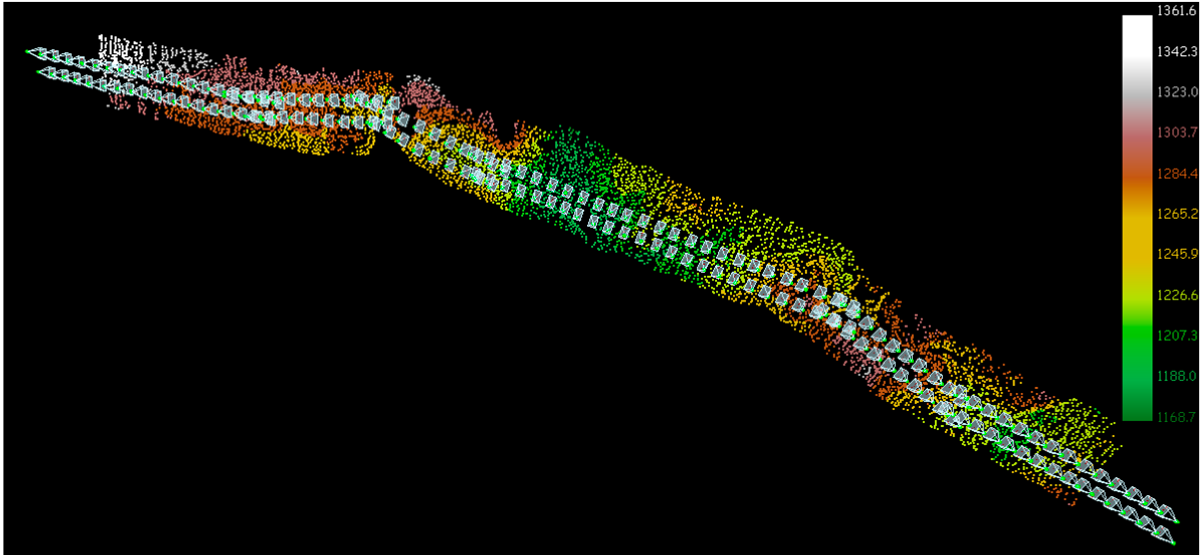
Figure 12.
Tie point distribution in images. The dashed rectangles are images. The blue dots are tie points from inter-strips and the pink dots are tie points from the same strip.
Figure 12.
Tie point distribution in images. The dashed rectangles are images. The blue dots are tie points from inter-strips and the pink dots are tie points from the same strip.

Figure 13.
Distribution of the ground control points (GCPs) and check points. The dashed rectangles are images. The red triangles are GCPs and the green triangles are check points.
Figure 13.
Distribution of the ground control points (GCPs) and check points. The dashed rectangles are images. The red triangles are GCPs and the green triangles are check points.
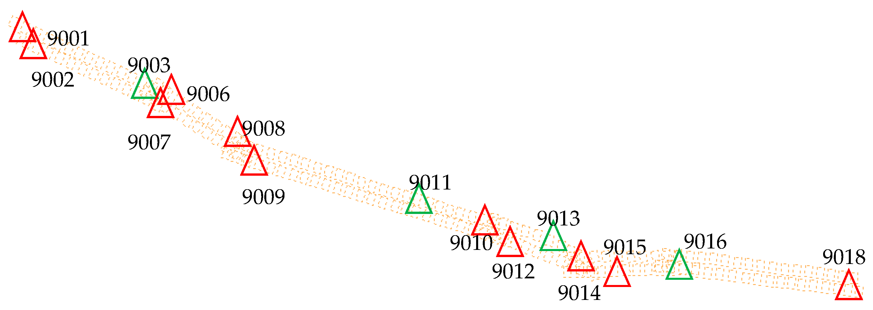
Figure 14.
The location and image measurement of GCP No. 9012. (a) The location of No. 9012; (b) The image measurement of No. 9012; the red crosses represent the location of the GCP in the images.
Figure 14.
The location and image measurement of GCP No. 9012. (a) The location of No. 9012; (b) The image measurement of No. 9012; the red crosses represent the location of the GCP in the images.

Figure 15.
Registration of a 2D vector and epipolar images of the power line.

Figure 16.
Three-dimensional reconstruction of the power line corridor and the distribution of obstacles.
Figure 16.
Three-dimensional reconstruction of the power line corridor and the distribution of obstacles.
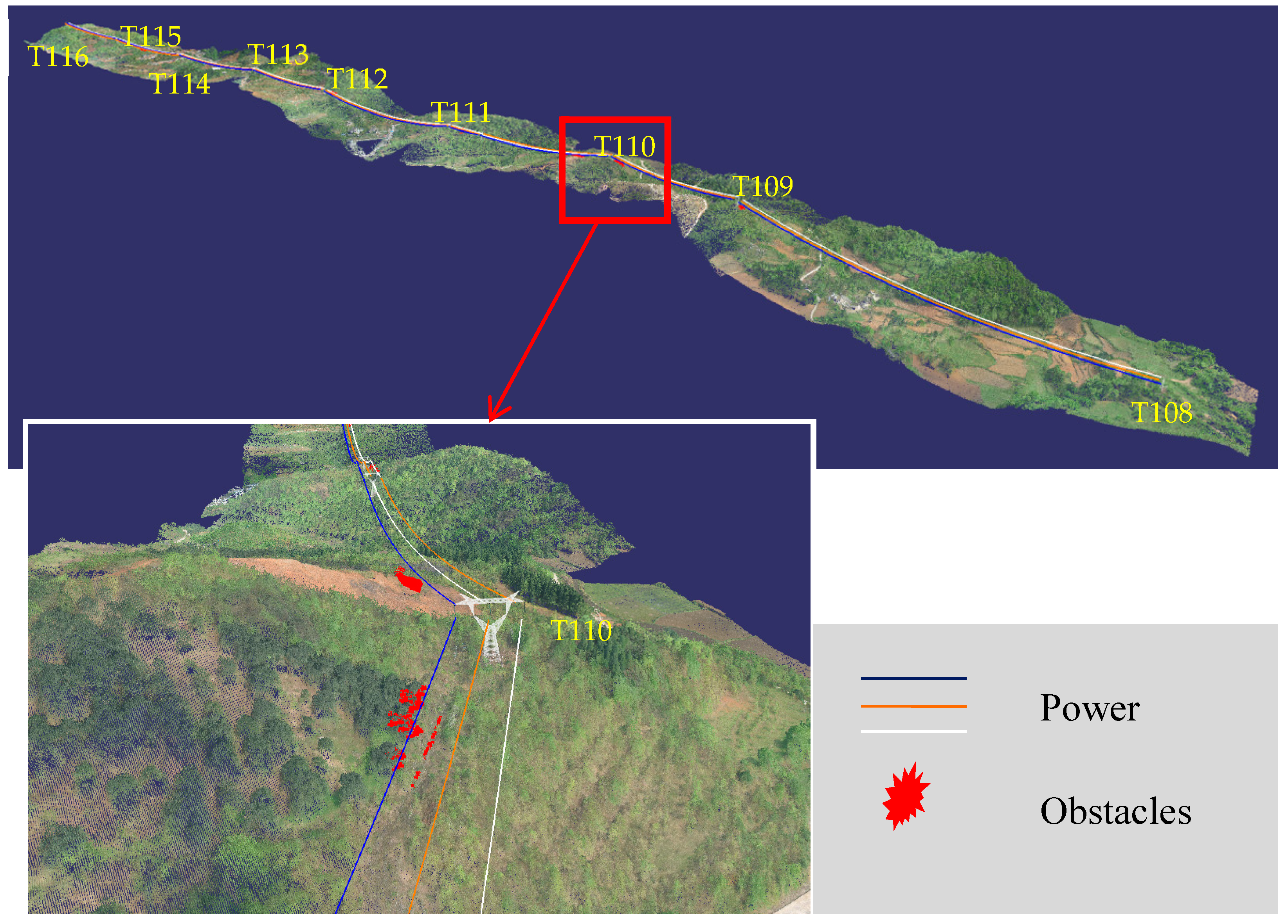
Figure 17.
Diagram of the profile analysis results of the power line corridor between T109 and T110. (a) Profile of the power line and the ground; (b) Distance between the power line and the ground.
Figure 17.
Diagram of the profile analysis results of the power line corridor between T109 and T110. (a) Profile of the power line and the ground; (b) Distance between the power line and the ground.

Table 1.
The coordinate differences of check points from in-strip stereo image pair (unit: m).
| Check Point No. | Stereo No. | Coordinate Difference | ||
|---|---|---|---|---|
| Easting | Northing | Elevation | ||
| 9003 | DSC_8780-DSC_8781 | 0.115 | −0.019 | 0.327 |
| DSC_8781-DSC_8782 | −0.080 | 0.043 | 0.324 | |
| DSC_8782-DSC_8783 | 0.082 | −0.038 | 0.294 | |
| DSC_8809-DSC_8810 | 0.125 | 0.052 | 0.212 | |
| DSC_8810-DSC_8811 | 0.046 | 0.070 | −0.183 | |
| DSC_8811-DSC_8812 | −0.052 | −0.106 | −0.280 | |
| 9011 | DSC_8820-DSC_8821 | −0.132 | −0.062 | 0.058 |
| DSC_8821-DSC_8822 | −0.049 | −0.081 | 0.214 | |
| DSC_8842-DSC_8843 | −0.089 | −0.053 | −0.194 | |
| 9013 | DSC_8928-DSC_8929 | 0.072 | 0.154 | 0.255 |
| DSC_8929-DSC_8930 | −0.071 | −0.026 | 0.283 | |
| DSC_8948-DSC_8949 | 0.082 | −0.017 | 0.223 | |
| DSC_8949-DSC_8950 | −0.090 | 0.037 | 0.176 | |
| DSC_8952-DSC_8953 | 0.088 | −0.034 | −0.265 | |
| DSC_8973-DSC_8974 | −0.083 | 0.036 | 0.157 | |
| 9016 | DSC_8960-DSC_8961 | 0.009 | 0.086 | −0.153 |
| DSC_8987-DSC_8986 | 0.011 | 0.166 | −0.298 | |
| DSC_8986-DSC_8985 | −0.004 | −0.097 | −0.385 | |
| DSC_8985-DSC_8984 | −0.039 | 0.058 | −0.185 | |
| DSC_9023-DSC_9022 | −0.017 | −0.115 | 0.090 | |
| DSC_9022-DSC_9021 | −0.017 | −0.057 | 0.275 | |
| DSC_9021-DSC_9020 | −0.004 | −0.122 | 0.078 | |
| Root mean square error of the coordinate difference | 0.073 | 0.081 | 0.233 | |
Table 2.
The coordinate differences of check points from inter-strip stereo image pair (unit: m).
| Check Point No. | Stereo No. | Coordinate Difference | ||
|---|---|---|---|---|
| Easting | Northing | Elevation | ||
| 9003 | DSC_8780-DSC_8809 | 0.047 | 0.055 | −0.217 |
| DSC_8781-DSC_8810 | 0.038 | 0.046 | −0.205 | |
| DSC_8782-DSC_8811 | 0.065 | 0.063 | −0.250 | |
| DSC_8783-DSC_8812 | 0.080 | 0.121 | −0.209 | |
| 9011 | DSC_8820-DSC_8842 | −0.016 | −0.056 | 0.194 |
| DSC_8821-DSC_8843 | −0.123 | −0.064 | 0.125 | |
| DSC_8822-DSC_8843 | −0.038 | −0.078 | 0.203 | |
| 9013 | DSC_8928-DSC_8948 | −0.156 | 0.058 | 0.305 |
| DSC_8929-DSC_8949 | −0.080 | 0.122 | 0.232 | |
| DSC_8930-DSC_8950 | −0.101 | 0.047 | 0.058 | |
| DSC_8952-DSC_8973 | 0.084 | −0.076 | 0.219 | |
| DSC_8953-DSC_8974 | 0.090 | −0.100 | 0.240 | |
| 9016 | DSC_8960-DSC_8983 | −0.055 | −0.112 | −0.141 |
| DSC_8961-DSC_8983 | −0.040 | 0.097 | −0.286 | |
| DSC_8987-DSC_9023 | 0.094 | −0.110 | −0.225 | |
| DSC_8986-DSC_9022 | −0.018 | 0.068 | −0.166 | |
| DSC_8985-DSC_9021 | 0.009 | 0.079 | −0.187 | |
| DSC_8984-DSC_9020 | 0.004 | −0.109 | 0.050 | |
| Root mean square error of the coordinate difference | 0.075 | 0.085 | 0.205 | |
Table 3.
Distribution of the elevation differences among sampling points in the power line profile (unit: m).
Table 3.
Distribution of the elevation differences among sampling points in the power line profile (unit: m).
| Elevation of Manual Measurement | Elevation of the PLAMEC | Elevation Difference |
|---|---|---|
| 1261.858 | 1261.906 | 0.048 |
| 1261.571 | 1261.397 | −0.174 |
| 1315.674 | 1315.705 | 0.031 |
| 1316.065 | 1315.822 | −0.243 |
| 1279.093 | 1279.090 | −0.003 |
| 1278.859 | 1279.044 | 0.185 |
| 1248.168 | 1248.040 | −0.128 |
| 1248.187 | 1248.217 | 0.030 |
| 1248.440 | 1248.560 | 0.120 |
| 1247.950 | 1247.721 | −0.229 |
| 1264.729 | 1264.682 | −0.047 |
| 1264.611 | 1264.793 | 0.182 |
| 1298.366 | 1298.251 | −0.115 |
| 1298.145 | 1298.316 | 0.171 |
Root mean square error of the elevation difference: 0.148 m.
Table 4.
Distribution of obstacles within the power line corridor (safety distance threshold: 6.5 m).
Table 4.
Distribution of obstacles within the power line corridor (safety distance threshold: 6.5 m).
| Tower Section | Position of the Obstacles (m) | Distance Between the Obstacles and the Power Line (m) | Distance Difference | |
|---|---|---|---|---|
| Proposed Method | Field Measurement | |||
| T108~T109 | 674.0–679.0 | 5.945 | 6.3 | 0.355 |
| T109~T110 | 375.5–400.0 | 4.626 | 4.8 | 0.174 |
| T110~T111 | 84.0–116.0 | 5.012 | 5.4 | 0.388 |
| 142.0–144.5 | 5.820 | 5.4 | −0.420 | |
| T111~T112 | 93.5–96.0 | 6.021 | 5.9 | −0.121 |
| 112.0–122.5 | 5.161 | 5.3 | 0.139 | |
| T112~T113 | 584.0–600.0 | 6.113 | 5.9 | −0.213 |
| T115~T116 | 235.0–247.0 | 5.889 | 5.5 | −0.389 |
Root mean square error of the distance difference: 0.319 m.
© 2017 by the authors. Licensee MDPI, Basel, Switzerland. This article is an open access article distributed under the terms and conditions of the Creative Commons Attribution (CC BY) license (http://creativecommons.org/licenses/by/4.0/).
Share and Cite
MDPI and ACS Style
Zhang, Y.; Yuan, X.; Li, W.; Chen, S. Automatic Power Line Inspection Using UAV Images. Remote Sens. 2017, 9, 824. https://doi.org/10.3390/rs9080824
AMA Style
Zhang Y, Yuan X, Li W, Chen S. Automatic Power Line Inspection Using UAV Images. Remote Sensing. 2017; 9(8):824. https://doi.org/10.3390/rs9080824
Chicago/Turabian StyleZhang, Yong, Xiuxiao Yuan, Wenzhuo Li, and Shiyu Chen. 2017. "Automatic Power Line Inspection Using UAV Images" Remote Sensing 9, no. 8: 824. https://doi.org/10.3390/rs9080824
Note that from the first issue of 2016, this journal uses article numbers instead of page numbers. See further details here.