Evaluating Sentinel-2 and Landsat-8 Data to Map Sucessional Forest Stages in a Subtropical Forest in Southern Brazil

Abstract

Studies designed to discriminate different successional forest stages play a strategic role in forest management, forest policy and environmental conservation in tropical environments. The discrimination of different successional forest stages is still a challenge due to the spectral similarity among the concerned classes. Considering this, the objective of this paper was to investigate the performance of Sentinel-2 and Landsat-8 data for discriminating different successional forest stages of a patch located in a subtropical portion of the Atlantic Rain Forest in Southern Brazil with the aid of two machine learning algorithms and relying on the use of spectral reflectance data selected over two seasons and attributes thereof derived. Random Forest (RF) and Support Vector Machine (SVM) were used as classifiers with different subsets of predictor variables (multitemporal spectral reflectance, textural metrics and vegetation indices). All the experiments reached satisfactory results, with Kappa indices varying between 0.9, with Landsat-8 spectral reflectance alone and the SVM algorithm, and 0.98, with Sentinel-2 spectral reflectance alone also associated with the SVM algorithm. The Landsat-8 data had a significant increase in accuracy with the inclusion of other predictor variables in the classification process besides the pure spectral reflectance bands. The classification methods SVM and RF had similar performances in general. As to the RF method, the texture mean of the red-edge and SWIR bands were considered the most important ranked attributes for the classification of Sentinel-2 data, while attributes resulting from multitemporal bands, textural metrics of SWIR bands and vegetation indices were the most important ones in the Landsat-8 data classification.

1. Introduction

Tropical forests are among the most complex ecosystems on Earth, playing crucial roles in biodiversity conservation and in ecology dynamics at global scale [1]. According to Viana and Tabanez [2], the Atlantic Rain Forest is one of the most endangered tropical ecosystems in the world, owning merely less than 16% of its original area [3]. This biome has been particularly affected by anthropogenic factors, such as industrial activities and urbanization, which brought changes in land cover and land use. As a result, forest remnants are sparsely found and present different degradation levels and successional forest stages.

Despite these threats, the Atlantic Forest and its associated ecosystems (sandbanks and mangroves) are still rich with respect to biodiversity, accounting for a meaningful share of the national biodiversity, with high rates of endemism [4]. As reported by these authors, this complex biome contains greater species diversity than that observed in the Amazon Forest. This species richness, the extremely high rates of endemism and the small percentage of this forest remnants led Myers et al. [5] to classify the Atlantic Forest among the main global biodiversity hot spots.

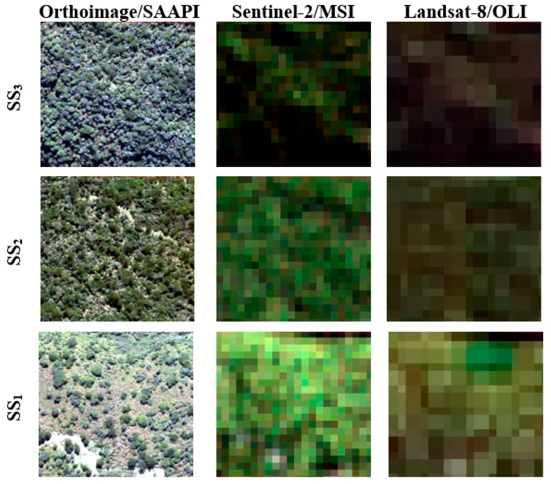
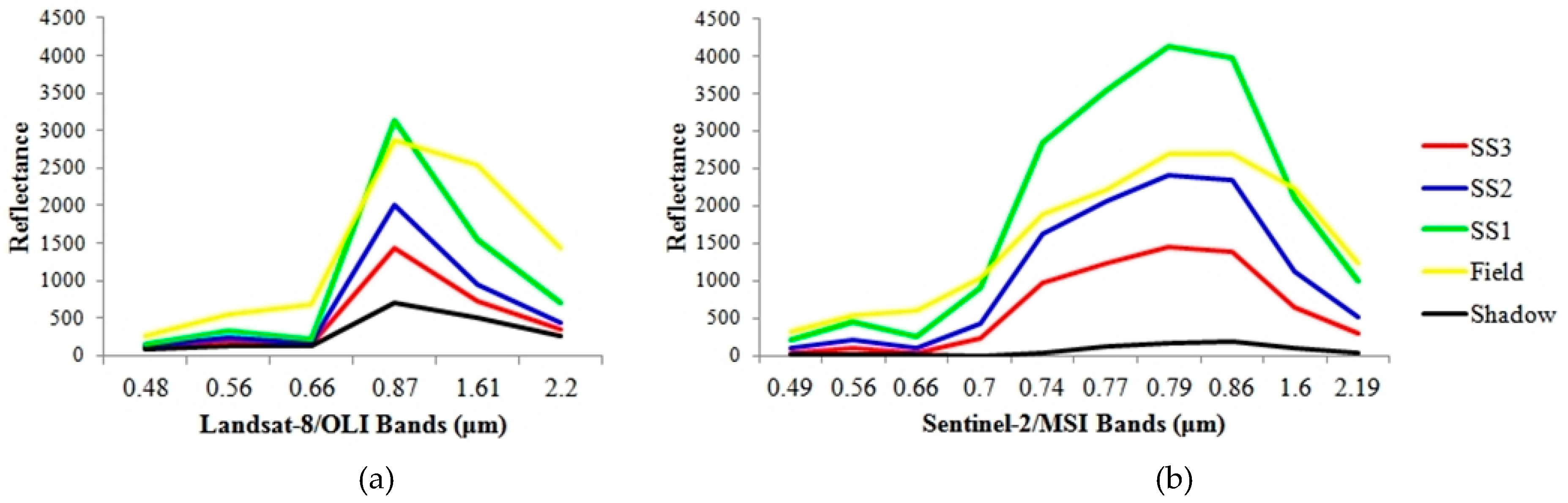
In a general way, with the help of field measurements, vegetation can be grouped into three stages of forest succession: early stage (SS₁), intermediate stage (SS₂) and advanced stage (SS₃) [6,7,8,9]. Each of them owns particular characteristics with regard to species composition and vegetation structure [7]. In the case of the Atlantic Forest, the successional stages are dealt with and regulated in different ways by the Brazilian environmental protection legislation, for instance in the case of the Atlantic Forest Law (Law Nr. 11.428/2006) [10]. In this way, mapping these stages represents a fundamental task to support studies with manifold applications, besides management, surveillance and environmental conservation initiatives [3], hence allowing quantitatively and qualitatively assessing the forest remnants as well as their spatial distribution.

In the latest decades, mankind has witnessed a remarkable advancement of space technologies targeted to monitoring forest resources. The recent refinement of both spatial and spectral settings of orbital sensors and the increasing improvement in the classification algorithms have strengthened the usability of remote sensing data as a source for land cover and land use mapping [11]. Orbital remote sensing tends to be considerably more advantageous when compared to conventional in situ mapping, not only because these data are systematically acquired, allowing their application at large scales, but also because they involve a less capital- and labor-intensive acquisition [12].

Nevertheless, mapping forest successional stages by means of remote sensing imagery imposes further challenges in the classification process, since the reflectance spectra of the concerned classes are very similar [13]. Several authors have committed themselves to characterize and classify successional stages of vegetation using remotely sensed imagery [8,13,14,15,16,17,18,19,20,21]. As stated by Lu et al. [8], the selection of appropriate variables and the development of refined algorithms are the two core research topics to be pursued in order to improve the performance of vegetation classification.

In addition to this, the new generation of Earth observation satellites offers a considerable improvement in the spectral, radiometric and spatial resolutions of their payloads. The quality of data acquired by these satellites associated with shorter revisit times allows the inclusion of temporal information on the vegetation phenology in the classification process. The Landsat satellite series has been providing valuable data sets for monitoring and mapping the Earth surface for over 40 years [22]. The Landsat-8 satellite, launched in 2013, enhanced the imaging capacity of this series, introducing new spectral bands in the blue and short-wave infrared (SWIR) ranges, as well as improving the sensor signal/noise ratio and the images radiometric resolution [23]. The Operational Land Imager (OLI) sensor supplies optical images with 30 m of spatial resolution, eight spectral bands and 16 days of temporal resolution [24].

Sentinel-2, a multispectral sensor of medium spatial resolution produced by the European Space Agency (ESA), was conceived to assure the continuity of global data coverage of the Earth surface accomplished by Landsat and SPOT satellites series. This mission was launched in 2015 and presents a wide swath (290 km), good revisit capacity (five days, with two satellites), high and medium spatial resolution (10, 20 and 60 m) and a relatively high number of bands (13 spectral bands) [25]. Considering that it is a newly launched satellite, studies to investigate its potential for forest applications are still few and incipient. Among works published using simulated or pre-operational data of this satellite, we ought to mention the paper of Frampton et al. [26], who used simulated Sentinel-2 data for estimating biophysical variables of vegetation; Immitzer et al. [27], who tested the use of Sentinel-2 data for mapping agricultural and tree species in Austria and Germany; and Addabbo et al. [28], who verified the capacity of these data for vegetation monitoring.

Besides the imagery properness, the right choice of classification methods is also decisive for a successful land cover and land use mapping [29]. Nonparametric methods, such as those based on machine learning, have gained great attention for classifying species and forest typologies [30]. Among the most often used ones, K-Nearest Neighbors (KNN), Artificial Neural Networks (ANN), Decision Trees (DT), Random Forest (RF) and Support Vector Machine (SVM) are to be mentioned. According to Prasad et al. [31], DTs are sensitive to small changes in the training data set and have been said to be occasionally unstable, for they tend to overfit the model to the training data. Naidoo et al. [32] report that it is difficult to set the ideal value of K for the KNN classifier, while ANN is a technique that demands greater computational processing due to its high level of complexity. Therefore, among the state-of-the-art nonparametric algorithms, both RF and SVM machine learning methods have been on the spot light due to their effectiveness in images classification [11]. This includes their ability to synthesize regression or classification functions based on discrete or continuous data sets, insensitivity to noise or overtraining, and ability to deal with unbalanced data sets [33].

Several studies compared the performance of the above-mentioned classifiers among themselves or in relation to other nonparametric classifiers, with the intent of classifying either land cover/land use [11], agricultural areas [34] or forests [30,35,36,37]. The authors of such works reached no consensus, for the performance of a classifier is always dependent on the particular test sites characteristics, on the type and quality of the remotely sensed data, and also on the number and general aspects of the classes of interest. Adam et al. [11] and Gosh et al. [37], for instance, found no statistically significant difference between the results of RF and SVM. In the same line, Ferét and Asner [36] acknowledged that no unique optimal classifier was found for all conditions tested, but emphasized the possibility of improving SVM classification with a better optimization of its parameters. Li et al. [34], on their turn, concluded that RF attained the best results in comparison with SVM and showed to be more stable in face of changes in the segmentation parameters and in the attributes selection. In contrast to these authors, Dalponte et al. [35] and Deng et al. [30] state the superior performance of SVM and Quadratic SVM (QSVM), respectively, as compared to RF. According to Dalponte et al [35], RF has the advantage of requiring less parameters to be estimated and a reduced computational cost. Nevertheless, when RF is applied to unbalanced training data, it tends to focus more on the prediction accuracy of prevailing classes, which generally results in low accuracy of less representative classes.

We should point out that previous investigations have shown that GEOBIA approaches improve classification accuracies in forest applications [21,36,38,39,40]. As highlighted by Ma et al. [38], although GEOBIA is often applied to medium spatial resolution imagery, high spatial resolution remote sensing images still remain as the most frequently used data source in such applications. In the current work, besides using medium spatial resolution imagery, we specifically deal with a limited number of classes (five), and in this particular case, the literature reports that GEOBIA and pixel-based classifications tend to attain similar accuracies [41,42]. Weih and Riggan [41] compared the performance of a pixel-per-pixel classification with GEOBIA applied to high resolution ortophotos and SPOT-5 medium resolution imagery for the discrimination of 13 land cover and land use classes. The authors concluded that the use of GEOBIA did not present significantly different results from those derived from the pixel-based classification when applied to the SPOT-5 10 m spatial resolution images. Lu et al. [9] comparatively evaluated the maximum likelihood classifier (MLC), ANN, KNN, SVM, DT and GEOBIA applied to Landsat-5/TM and ALOS PALSAR medium resolution images for the classification of three successional vegetation stages in the Brazilian Amazon Forest. The authors came to the conclusion that the classifiers performance varied as a function of the data sets used, and that GEOBIA had a similar performance in relation to the other methods. Meroni et al. [42] tested the accuracy of the RF classifier and different classification set-ups, varying the spatial resolution (the original 30 m vs. the pan-sharpened 15 m) and image acquisition dates (during the wet season, the dry season and a combination of the two) for seven classes involving different forest types and species. The best overall accuracy (84%) was achieved using the pan-sharpened data from the two seasons. The authors compared pixel-based and GEOBIA approaches and concluded that GEOBIA achieved the same overall accuracy in the specific presence of such a small number of classes.

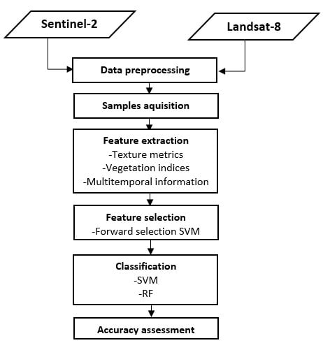
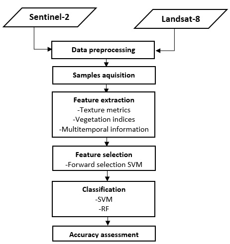
Considering the research above, the general goal of this work is to evaluate the performance of both Landsat-8 and Sentinel-2 imagery for the semiautomatic pixel-based classification of successional stages in a particular subtropical Atlantic Forest environment. The specific goals are: (1) successional stages mapping with Landsat-8 and Sentinel-2 data; (2) verification of the contribution of textural metrics, vegetation indices and multitemporal data for the classification of successional stages; and (3) comparison of the performance of two machine learning algorithms (RF and SVM).

2. Materials and Methods

The methodology framework developed for this research is shown in Figure 1.

2.1. Study Area

The study area extends over 900 ha of a subtropical portion of the Atlantic Rain Forest. It is located in the northern region of São Joaquim National Park (in the Brazilian southern State of Santa Catarina), at an elevation of 1638 m above sea level (Figure 2). The vegetation consists of patches of Mixed Ombrophilous Forest amidst Highland Fields and Cloud Forests [43]. According to Faxina [43], the soil stratum is predominantly shallow, stony, presenting basalt and sandstone rock outcrops, with prevailing Neosol, Argisol and Cambisol soils dating back nearly 133 million years. The climate, according to Köppen’s classification, is Cfb, moist mesothermal with no clearly defined dry season, mild summers, often and severe freezes in winter, and mean temperature of 12 °C. The average annual rainfall is 1400 mm. The vegetation in the study area presents less marked climatic and phenological responses to seasonality [44,45].

2.2. Data Preprocessing

Two Landsat-8 OLI scenes, WRS 220/080 and 220/079, respectively dated from June and November 2016, both Level L1T geocoded and terrain corrected, were downloaded from the United States Geological Survey (USGS) website. Six multispectral bands were used for each of the two scenes (

Table 1. Spatial and spectral resolutions of Landsat-8/OLI and Sentinel-2/MSI.

Landsat-8/OLI (μm)	Band	Resolution (m)	Sentinel-2/MSI (μm)	Band	Resolution (m)
Band 2 (0.45–0.51)	Blue	30	Band 2 (0.46–0.52)	Blue	10
Band 3 (0.53–0.59)	Green	30	Band 3 (0.54–0.58)	Green	10
Band 4 (0.64–0.67)	Red	30	Band 4 (0.65–0.68)	Red	10
Band 5 (0.85–0.88)	NIR	30	Band 5 (0.7–0.71)	Red-edge-1	20
Band 6 (1.57–1.65)	SWIR-1	30	Band 6 (0.73–0.75)	Red-edge-2	20
Band 7 (2.11–2.29)	SWIR-2	30	Band 7 (0.76–0.78)	Red-edge-3	20
Band 8 (0.50–0.68)	Panchromatic	15	Band 8 (0.78–0.90)	NIR	10
			Band 8A (0.85–0.87)	NIR plateau	20
			Band 11 (1.56–1.65)	SWIR-1	20
			Band 12 (2.10–2.28)	SWIR-2	20

). Initially, the multispectral images were converted to surface reflectance values using the Fast Line-Of-Sight Atmospheric Analysis Of Spectral Hypercubes (FLAASH) algorithm, which also rendered available the reflectance curves visualization of the classes of interest. After this procedure, these bands were pansharpened with the panchromatic band by means of the Gram–Schmidt algorithm, resulting in multispectral bands with 15 m of spatial resolution. This operation was independently applied to both L8-OLI scenes.

The MultiSpectral Instrument (MSI) scenes of the Sentinel-2 mission were acquired from the Land Viewer (lv.eosda.com) website, dated from June and December 2016, both Level L1C geocoded (Table 1). All Sentinel-2 bands with 20 m of spatial resolution as well as all Landsat-8 pansharpened bands were resampled to 10 m using the nearest-neighbor interpolation algorithm, so as to enable comparisons among them without reducing the best spatial resolution (10 m) of Sentinel-2 Bands 2, 3, 4 and 8. Bands designed to atmospheric correction and to track clouds and water vapor from both sensors were disregarded in this work. Finally, the digital numbers in Sentinel-2 scenes were also converted to surface reflectance values using the FLAASH algorithm.

Although the vegetation in the study area presents reduced climatic and phenological seasonality, as previously stated, the observed reflectance varies with season due to changes in the solar illumination geometry caused by the Earth translation movement (

Table 2. Acquisition dates, solar elevation and azimuth angles of Landsat-8 and Sentinel-2 scenes.

Satellite	Scene	Acquisition Date	Solar Elevation (°)	Solar Azimuth (°)
Landsat-8	LC82200792016164LGN01	6/12/2016	31.07	33.81
Landsat-8	LC82200802016308LGN01	11/03/2016	61.44	67.49
Sentinel-2	S2A_tile_20160609_22JFQ_1	6/08/2016	33.19	29.67
Sentinel-2	S2A_tile_20161206_22JFQ_0	12/06/2016	67.07	82.86

). This variation in the solar angles at the moment of image acquisition may impact the amount of shadow present in the canopy, and, hence, the bidirectional reflectance distribution function (BRDF) [46].

2.3. Classes Definition and Samples Acquisition

After data preprocessing, the land cover classes were defined. In the sequence, samples acquisition was carried out with the aid of ROI (region of interest) polygons in ENVI 5.0 through a manual sampling strategy, in order to provide spectral, spatial, and textural signatures for each class [21]. The adopted classes in the study area and their respective number of pixels used for training were: vegetation at an early stage of recovery (SS₁) (200 pixels), vegetation at an intermediate stage of recovery (SS₂) (205 pixels), vegetation at an advanced stage of recovery (SS₃) (212 pixels), field (comprising bare soil and highland fens) (262 pixels), and shadow (119 pixels). Field visits for ground truth check were realized by Faxina [43]. This author basically employed a systematic distribution of sample units (SUs), with a grid resolution of 500 m × 500 m. In the SUs with a minimum forest share of 75%, parcels with a total area of 1200 m² (10 m of width by 30 m of length) have been allocated, where all individual trees with diameter at breast height (DBH) equal to or greater than 10 cm were catalogued in a field survey. The vegetation successional stage was defined according to criteria established by a federal resolution of the Brazilian National Council for the Environment (CONAMA, Res. Nr. 04/1994) [47].

The field survey revealed that in the SS₃ class, late succession species or primitive species of the Mixed Ombrophilous Forest are predominant, such as Clethra uleana, Drymis angustifolia, Myrcia palustris, Dicksonia sellowiana and those of the gender Ocotea sp. and Myrceugenia sp. As for the SS₂, some late succession species or primitive species are also found, such as Ocotea porosa and Dicksonia sellowiana, however pioneer or early succession species are also observed, such as Mimosa scabrella, Baccharis uncinella and Myrsine coriácea. The Araucaria angustifolia species is prevailing throughout the study area and presents both pioneer and late succession characteristics [48]. Currently, this species is at risk of extinction, which denotes the importance of granting priority for conservation of these areas.

The selection of samples was based on the fieldwork accomplished by Faxina [43], on the photointerpretation of orthoimages with a 0.39 m spatial resolution (Figure 3), collected by the Airborne System for Acquisition and Post-processing Images (SAAPI), consisting of digital multispectral cameras, and also on current images of Google Earth. Figure 3 presents examples of the three classes of vegetation successional stages, acquired by SAAPI orthoimages and the corresponding Sentinel-2 and Landsat-8 subscenes.

2.4. Feature Extraction and Selection

One of the goals of this work was exploring features (attributes) other than the single spectral bands alone, such as textural metrics, vegetation indices as well as the inclusion of multitemporal information in the classification process. Texture-based methods are commonly used for effectively incorporating spatial information in image interpretation. Textural metrics based on the gray-level co-occurrence matrix (GLCM), proposed by Haralick et al. [49], have been extensively used for land cover classification [8,50,51] and for enhancing the discrimination of vegetation classes [52,53]. Previous studies conducted by Sothe et al. [20] showed that the texture mean, contrast and dissimilarity were considered the most important ones for identifying vegetation successional stages in a patch of the Atlantic Forest, which justifies their use in the present work.

The GLCM-based textural analysis requires setting four parameters: window size, spectral bands, level of quantization, and the spatial component, this latter corresponding to the distance between pixels and the angle (direction). The window size has an impact on the GLCM textural metrics performance for classifying land cover. Small windows may amplify differences and increase the noise content in the texture image, while larger windows cannot effectively extract texture information due to smoothing the texture variation [54,55]. Preliminary tests in the same study area and also using a L8 image conducted by Sothe et al. [20] indicated that textural parameters extracted by a 7 × 7 window size, in the southwest direction and at the level of quantization of 64 bits were the most appropriate for separating the classes of interest in images of both sensors. The textural metrics were calculated for all spectral bands of each sensor.

Vegetation indices are also useful for characterizing forest typologies. The seminal indices were meant to enhance the strong reflectance of vegetation in the near infrared (NIR) region in relation to its marked absorption by chlorophyll in the red region of the electromagnetic spectrum in order to quantify the vegetation greenness, such as the Normalized Difference Vegetation Index (NDVI) or the Difference Vegetation Index (DVI), calculated as a simple difference between the spectral reflectance in the NIR and red ranges.

More recently, with the advent of new multispectral sensors, some refinements were made possible in the conception of these indices, such as the Optimized Soil Adjusted Vegetation Index (OSAVI), which employs a soil adjustment coefficient (0.16) to minimize NDVI’s sensitivity to variation in soil background under a wide range of environmental conditions. Two new indices based on the NDVI were created: the Green-Red Vegetation Index (GRVI), which replaces the NIR band by the green band, relying on the fact that the NDVI presents saturation problems in dense forest canopies, mainly due to the spectral reflectance of vegetation in the NIR region, which makes this new index insensitive to certain changes; and the Green Normalized Vegetation Index (GNDVI), which on its turn replaces the red band by the green band, since this channel is more sensitive to chlorophyll than the red channel. Recent multispectral sensors also allowed the calculation of the Red-edge Normalized Difference Vegetation Index (NDVIRed-edge) [56], which is composed by the spectral response of a band located in the red-edge region. According to Hatfield et al. [57], the usage of the green and red-edge channels avoid saturation and the concurrent loss of sensitivity to certain values of chlorophyll, besides being generally preferred because they are more sensitive to moderate and high contents of chlorophyll. The Normalized Difference Infrared Index (NDII) is also to be cited, which is used to indicate the vegetation moisture conditions [58]. The indices described in

Table 3. Vegetation indices and respective equations and references.

Index	Equation	Reference
Normalized Difference Vegetation Index	NDVI = $\frac{{\rho }_{nir}-{\rho }_r}{{\rho }_{nir}+{\rho }_r}$	Rouse et al. [59]
Difference Vegetation Index	DVI =${\rho }_{nir}-{\rho }_r$	Richardson and Wiegand [60]
Green Normalized Vegetation Index	GNDVI = $\frac{{\rho }_{nir}-{\rho }_g}{{\rho }_{nir}+{\rho }_g}$	Gitelson et al. [61]
Normalized Difference Vegetation Index Red-edge	NDVIRed-edge = $\frac{{\rho }_{redge}-{\rho }_r}{{\rho }_{redge}+{\rho }_r}$	Gitelson and Merzlyak [56]
Green-Red Vegetation Index	GRVI = $\frac{{\rho }_g-{\rho }_r}{{\rho }_g+{\rho }_r}$	Tucker [62]
Optimized Soil Adjusted Vegetation Index	OSAVI = $\frac{{\rho }_{nir}-{\rho }_r}{{\rho }_{nir}+{\rho }_{r+0.16}}$	Rondeaux et al. [63]
Normalized Difference Infrared Index	NDII = $\frac{{\rho }_{nir}-{\rho }_{swir}}{{\rho }_{nir}+{\rho }_{swir}}$	Hardisky et al. [64]

$\rho$, spectral reflectance; r, red; g, green; nir, near infrared; swir, short-wave infrared.

were computed using the bands of the two sensors (OLI and MSI), with the exception of the NDVIRed-edge, which is only available for the MSI sensor.

Both the textural metrics and the vegetation indices were computed for the June OLI and MSI scenes, corresponding to the fall season in the Southern Hemisphere. However, with the purpose of verifying the contribution of multitemporal information in the classification, similar to the work conducted by Clark and Kilham [65], the spectral bands of spring were added to some experiments, corresponding to the November OLI scene and the December MSI scene. We should clarify that it was not possible to obtain images from the same date for both sensors due to the presence of clouds over the study area.

For the sake of clarity, each experiment was named as a function of the group of variables and sensor used in the classification process (

Table 4. Description of the classification experiments according to the employed group of predictor variables (spectral bands, textural metrics, and vegetation indices).

Group	Spectral Bands “Fall”	Texture “Fall” Bands	Vegetation Indices	Spectral Bands “Spring”	Total Number of Variables
G1-L8	2, 3, 4, 5, 6, 7	-	-	-	6
G2-L8	2, 3, 4, 5, 6, 7	Mean, cont., diss.1	-	-	24
G3-L8	2, 3, 4, 5, 6, 7	-	All2	-	12
G4-L8	2, 3, 4, 5, 6, 7	-	-	2, 3, 4, 5, 6, 7	12
G5-L8	2, 3, 4, 5, 6, 7	Mean, cont., diss.1	All2	2, 3, 4, 5, 6, 7	36
G6-L8	Bands selected using the forward selection—SVM				13
G1-S2	2, 3, 4, 5, 6, 7, 8, 8A, 11, 12	-	-	-	10
G2-S2	2, 3, 4, 5, 6, 7, 8, 8A, 11, 12	Mean, cont., diss.1	-	-	50
G3-S2	2, 3, 4, 5, 6, 7, 8, 8A, 11, 12	-	All	-	17
G4-S2	2, 3, 4, 5, 6, 7, 8, 8A, 11, 12	-	-	2, 3, 4, 5, 6, 7, 8, 8A, 11, 12	20
G5-S2	2, 3, 4, 5, 6, 7, 8, 8A, 11, 12	Mean, cont., diss.1	All	2, 3, 4, 5, 6, 7, 8, 8A, 11, 12	57
G6-S2	Bands selected using the forward selection—SVM				16

¹ Mean, texture mean; cont., contrast; diss., dissimilarity of all spectral bands acquired in “fall”. ² All the vegetation indices shown in Table 3, except the NDVIRed-edge. L8, Landsat-8; S2, Sentinel-2.

).

Pal and Foody [66] mention that the use of a smaller number of variables may result in an accuracy equal to or even superior in comparison with the use of large data sets, besides providing potential advantages in terms of data storing and processing costs. In this way, feature selection is considered an important step within a classification process because it improves the performance of the classifier and reduces the complexity of the computation by removing redundant information [67]. Feature selection algorithms are separated into three categories: filters, wrappers and the embedded techniques [68,69]. Wrappers utilize the learning machine of interest as a black box to score subsets of variables according to their predictive power [67,70]. This approach tend to perform better in selecting features, since they take the model hypothesis into account by training and testing it in the feature space [69]. Many previous studies adopted the SVM as the learning scheme, due to its superiority when compared to other classifiers [67,70,71]. When comparing seven feature selection algorithms for land cover classification using the SVM and RF methods, Ma et al. [67] found that the SVM Recursive Feature Elimination (SVM-RFE) wrapper was appropriate for both classifiers, SVM and RF. A novel wrapper approach has also been suggested by Ma et al. [72], which involves the integration of: (i) feature importance rank using gain ratio; and (ii) feature subset evaluation using a polygon-based tenfold cross-validation within a support vector machine (SVM) classifier. As reported by the authors, this approach yielded promising results, considerably increasing the final classification overall accuracy.

Considering this, a wrapper approach was tested for feature selection [73], which can either be based on a forward selection or on a backward elimination. The former one was chosen, in which selection starts with an empty feature set and the SVMs are then trained for each attribute individually. The attribute corresponding to the SVM with the best performance is then selected. At the second iteration, the SVMs are trained for each pair of attributes, which consist of the best previously executed characteristic and an additional attribute. Again, the pair of attributes corresponding to the SVM with the best performance is then selected. This step is repeated until all attributes are selected or a stop criterion defined by the user is met. This results in a list containing the added attributes one by one and their respective performances [74]. The SVM forward selection algorithm requires setting two parameters: the number of cross-validations and the stop criterion. We kept the standard settings of 3 for the first parameter and 0.1 for the second parameter. It is worth stressing that the attributes selection was applied in the experiments containing all variables (G5-L8 and G5-S2). The best evaluated attributes subset was employed in the last experiments described in Table 4 (G6-L8 and G6-S2).

2.5. Semiautomatic Classification

The variables selected for each experiment, as shown in Table 4, were grouped in only one file and each group was subject to two classifiers: RF and SVM, both of them available in the open source platform ENMap-Box [75]. Random Forest (RF) is a technique conceived by Breiman [33], as a means to improve the accuracy of classification and regression trees through the combination of a great number of random subsets of trees. Each tree contributes with only one vote and the final classification is determined by the majority of votes taking into account all the forest trees.

In the RF algorithm there are two parameters to be defined: the number of variables in the random subset at each node (mtry) and the number of trees (ntree). Rodriguez-Galiano et al. [76] realized an empirical evaluation regarding the parameter “number of trees” and concluded that differences in the classification accuracy above a hundred trees are meaningless. In this study, this classifier was preliminarily tested with 100, 500 and 1000 trees. It was found that increasing the number of trees from 100 to 500 led to a small improvement in the classification result, while changing from 500 to 1000 trees considerably increased the processing time with no corresponding increase in accuracy. In face of this, we opted for using 500 trees in all experiments. Regarding the mtry parameter, the default value was kept, which corresponds to the square root of the total number of bands used in each experiment [33].

In order to estimate classification errors, the RF algorithm collects around 2/3 of the training data with replacement, while the remaining data are left out-of-bag (OOB). These OOB samples are assigned to trees that have not yet been used, and the difference between the expected and the real class is used to assess the classification accuracy [65]. When compared to cross-validation, the OOB error is unbiased and represents a good estimate for the generalization error. As the number of trees increases, the OOB error decays and tends to converge to a threshold [77].

Besides estimating the error, OOB samples were also used for computing the raw and normalized importance of each variable in the classification process. These samples are exchanged with the respective variable and suppressed from each tree, and the accuracies are then computed. Next, the accuracies of the exchanged OOB samples are subtracted from the accuracies of the original samples. The mean of the differences in accuracies of a variable corresponds to its raw importance. The ratio of the raw importance to its respective standard deviation results in the normalized importance of the concerned variable. A high value for the normalized importance means that the variable owns a massive importance for the whole random forest and the opposite holds true as well [77]. G5-L8 and G5-S2 were used for estimating the normalized importance of variables, given that all variables have been included in these experiments.

The SVM algorithm [78] is a supervised machine learning classifier, trained to find the optimal separating hyperplane by minimizing the upper limit of the classification error [11]. For mapping not linearly separable classes, four kernel functions of SVM are often used: linear, polynomial, radial basis function (RBF) and sigmoid. In this work, the RBF was chosen, for its superiority in relation to the other functions has been demonstrated in several studies [79,80]. This kernel function has two user-defined parameters that can affect the classification accuracy [81]: cost (C), value used to fit classification errors in the training data set [11], and gamma (g). A high value of C may overfit the model to data, while the adjustment of the g parameter will have an influence on the shape of the separating hyperplane [82]. Both parameters, g and C, depend on the data interval and distribution and differ from one classification to another. A common strategy to find appropriate values for g and C, which has been adopted in this particular case, is a bidimensional grid search with internal validation [74].

2.6. Statistical Assessment of Results

For accuracy assessment, independent sets of random points were generated for each classification result in a two-stage process. Initially, irregular polygons were manually delimited for each class directly in the images of both sensors, based on field observations and using very high spatial resolution images as ancillary data. In a second stage, inside each of these polygons, a stratified random sampling was conducted, where 70 pixels were selected for each of the three vegetation successional stages, 50 pixels for field and 50 pixels for the shadow class (Figure 4). This procedure was repeated for each classification to maintain the independence among the validation data sets. The number of samples was defined according to the work of Congalton and Green [83], who recommend a minimum of 50 samples for maps of less than one million acres in size and fewer than 12 classes.

After the samples acquisition, confusion matrices were elaborated based on a cross-check between the classified maps and the validation samples. These matrices allowed the calculation of the following agreement indices: (a) overall accuracy (OA); (b) producer’s accuracy, (c) user’s accuracy; and (d) Kappa index [83]. The z test was applied to the Kappa indices of all classifications with a significance level of 5%, i.e., a confidence interval of 95%. The value of the normal distribution of z is obtained by the ratio of the difference between two given Kappa indices to the difference between their respective variances [84]. If z > 1.96, the test is significant and the null hypothesis is rejected, leading us to conclude that there exists significant difference between the obtained results.

3. Results

3.1. Feature Selection and Spectral Reflectance

Table 5. Subset with the best predictor variables for Landsat-8 (L8) and Sentinel-2 (S2) scenes provided by the SVM forward selection.

Data	Selected Attributes (Predictor Variables)															Accuracy (%)
L8	B2S	B6S	B7S	M2	M3	C3	M4	M5	D6	M7	D7	NDVI	OSAVI	-	-	-	99.25
S2	B2	B6	B8	B4S	B6S	M2	M3	M4	C5	D5	C6	D8	M11	D12	OSAVI	C3	100

M, texture mean; D, dissimilarity; C, contrast; BS, “spring” spectral bands.

shows the attributes selected by the SVM wrapper forward selection, which integrate the experiments G6-L8 and G6-S2. For the Landsat-8 data, the combination of 13 attributes achieved 99.25% of accuracy, while for the Sentinel-2 data, the maximum accuracy of 100% was reached with 16 attributes. According to the learning curve, it was observed that the inclusion of new attributes gradually increases the accuracy until the curve stabilizes at a level, over which the addition of new variables produces a small or even no difference in accuracy. Regarding the Landsat-8 data, this baseline is around 98% and 99.4% accuracy, while Sentinel-2 reaches 100% accuracy from the 16th iteration onwards. Cetin et al. [85] state that it is difficult to increase the accuracy of a classification after a certain point, which depends mainly on the complexity of the training data set, on the number of classes and on the adopted classification technique.

Three “spring” spectral bands were selected for the Landsat-8 data. No pure “fall” spectral bands were selected in this case, only textural metrics thereof derived. The SWIR bands had a particularly meaningful importance for this data set, given that two “spring” bands (B6S and B7S), three textural metrics (D6, M7, and D7), besides two vegetation indices (NDVI and OSAVI) extracted in this spectral region were selected. For the Sentinel-2 data, three “fall” bands and two “spring” bands were selected, together with textural metrics extracted in all spectral regions and the vegetation index OSAVI. In this case, information derived from the red-edge region is to be mentioned, considering that five metrics extracted in this range of the electromagnetic spectrum were selected (B6, B6S, C5, D5, and C6).

In order to visualize the spectral reflectance curves of the three vegetation successional stages for both data sets, spectral profiles were generated considering the mean spectral response of the training samples (Figure 5). It is possible to observe that in the visible region (0.48–0.66 μm) the successional stages present very similar surface reflectance values, while in the NIR region (0.7–0.87 μm) the stages tend to be more separable from each other. In the NIR range, the SS₁ presented relatively higher surface reflectance values than the other stages. This behavior is somehow expected, since with the canopy roughness increase in later successional stages, the reflectance in this spectral region decreases due to the mutual shading either of forest strata or of dominant treetops, which project themselves to the upper part of the forest canopy [86,87]. In the SWIR range (OLI-B6, OLI-B7, MSI-B11, and MSI-B12), the spectral differences are smaller, but the SS₁ also presented surface reflectance values slightly superior in comparison to the intermediate and advanced stages. In this case, the plenty amount of leaves in the later stages reduces the canopy reflectance due to the greater water presence, which dominates the vegetation spectral behavior in this spectral region [14,88]. Thus, it becomes evident that the use of Sentinel-2 data allows the generation of spectral curves with a greater level of detailing than the Landsat-8 data, in face of the availability of three spectral bands in the red-edge region (0.7–0.77 μm), besides another band in the near infrared plateau (0.86 μm). The addition of spectral bands in this latter region substantially improves the discrimination of vegetation physiognomies.

3.2. Variables Importance

The RF algorithm assesses the importance of each variable in the classification process by means of a specific measure [77]. The reckoning of this measure allows the identification of the most relevant information for the discrimination of the vegetation successional classes. According to Figure 6, in the experiments accomplished with both satellites data, the texture mean was one of the most important variables for the two data sets, mainly Sentinel-2. Considering that this metric aggregates contextual information through a 7 × 7 neighborhood, it smoothens the image, reducing the impact of noisy pixels, shadows or small clearings that are eventually found throughout the vegetation, thus also decreasing the spectral mixture at the pixel level. In this way, it helps the classifier in the task of discriminating the vegetation successional stages.

It can be observed that the most important texture means of this ranking were obtained from the SWIR bands (M6 and M7 in the Landsat-8 scenes, and M11 and M12 in the Sentinel-2 scenes), which are placed in the first two positions for the Sentinel-2 data set. The texture means derived from the two red-edge bands (M5 and M7) are also among the most important predictor variables for the Sentinel-2 scenes.

3.3. Mapping Results and Classification Accuracies

Table 6. Overall Accuracy (OA) and Kappa index for the classification experiments.

RF		Producer’s Accuracy					User’s Accuracy					OA (%)	Kappa
		Land Cover Classes					Land Cover Classes
		SS3	SS2	SS1	Field	Shadow	SS3	SS2	SS1	Field	Shadow
Experiment	G1-L8	87.1	88.6	91.4	100	100	96.8	80.5	91.4	100	100	92.6	0.91
	G2-L8	91.4	94.3	98.6	100	100	97.0	91.7	97.2	98	100	96.5	0.961
	G3-L8	95.7	90.0	94.3	100	98	93.1	90.0	95.7	100	100	95.2	0.94
	G4-L8	92.9	97.1	98.6	100	100	97.0	95.8	98.6	96.2	100	97.4	0.971
	G5-L8	90.0	92.9	95.7	100	100	96.9	86.7	95.7	100	100	95.2	0.94
	G6-L8	88.6	92.9	91.4	98	100	93.9	85.5	97.0	96.1	98	93.5	0.92
	G1-S2	97.1	91.4	98.6	100	100	93.2	95.5	98.6	100	100	97.1	0.961
	G2-S2	98.6	92.9	98.6	100	100	93.2	98.5	100	100	98	97.7	0.971
	G3-S2	95.7	88.6	97.1	100	100	90.5	92.5	98.6	100	100	95.8	0.951
	G4-S2	98.6	85.7	94.3	100	100	88.5	93.8	97.1	100	100	95.2	0.94
	G5-S2	97.1	91.4	98.6	100	100	93.2	95.5	98.6	100	100	97.1	0.961
	G6-S2	95.7	95.7	97.1	100	100	98.5	94.4	97.1	100	98	97.4	0.971
SVM		Producer’s Accuracy					User’s Accuracy					OA (%)	Kappa
		Land Cover Classes					Land Cover Classes
		SS3	SS2	SS1	Field	Shadow	SS3	SS2	SS1	Field	Shadow
Experiment	G1-L8	88.6	88.6	87.1	100	100	91.2	83.8	96.8	90.9	100	91.9	0.90
	G2-L8	95.7	88.6	97.1	100	98	94.4	95.4	94.4	94.3	100	95.5	0.94
	G3-L8	97.1	94.3	92.9	100	98	94.4	89.2	100	100	100	96.1	0.951
	G4-L8	90	88.6	98.6	100	100	90.0	93.9	100	94.3	96.2	94.8	0.94
	G5-L8	94.3	88.6	95.7	96	100	94.3	92.5	93.1	94.1	100	94.5	0.93
	G6-L8	94.3	94.3	97.1	100	98	95.7	94.3	97.1	96.2	100	96.5	0.96
	G1-S2	100	97.1	95.7	100	100	98.6	95.8	98.5	100	100	98.4	0.981
	G2-S2	92.9	92.9	92.9	100	100	92.9	92.9	100	94.3	96.2	95.2	0.94
	G3-S2	91.4	92.9	92.9	100	100	94.1	85.5	98.5	100	100	94.8	0.94
	G4-S2	98.6	84.3	98.6	100	100	93.2	100	93.2	94.3	100	95.8	0.951
	G5-S2	91.4	94.3	94.3	100	100	95.5	91.7	98.5	96.2	96.2	95.5	0.94
	G6-S2	95.7	91.4	100	100	96	95.7	95.5	93.3	100	100	96.5	0.95

¹ Best results that did not significantly differ among themselves.

shows the overall accuracy and Kappa index for each classifier and group of employed variables, and Figure 7 illustrates the overall accuracy achieved in each classification experiment. The best and worst performances were reached in the experiments that used only the pure spectral bands of Sentinel-2 and Landsat-8, respectively. The minimum OA (91.9%) and Kappa index (0.90) refer to the G1-L8 experiment associated with the SVM classifier; and the maximum OA (98.4%) and Kappa index (0.98) relate to the G1-S2 experiment also associated with SVM. The OA of G1-S2 was significantly superior to that of all experiments using Landsat-8 data, with the exception of experiments G2-L8 and G4-L8 associated with RF, and G3-L8 with SVM. These results show that, for the particular case of the Sentinel-2 data, the usage of further variables, such as vegetation indices, texture and multitemporal data, was not necessary for improving classification results. In the experiments executed with Landsat-8 data, the inclusion of additional variables considerably improved classifications when compared to the usage of spectral bands alone (G1-L8). For both classifiers (RF and SVM), there was a meaningful improvement in classification when textural metrics (G2-L8) or the “spring” spectral bands (G4-L8) were added. Another experiment worthy of mention regarding Landsat-8 data was G6-L8, run with SVM, in which only the bands derived from feature selection were used (Table 5). In this table, there are three “spring” spectral bands, thus highlighting the importance of multitemporal information in the scenes classification. One of the factors for explaining the outperformance of the classification relying on “spring” spectral bands is the difference in solar illumination geometry during image acquisition between the two considered seasons. In the scenes acquired in spring, the incident sun radiation arrives in a more perpendicular direction to the Earth surface, reducing the shadow effect caused by topography and variations in the forest canopy height, leading to better “illuminated” pixels.

Among the experiments with Sentinel-2 data, G1-S2 was significantly superior to G2-S2, G3-S2 and G5-S2 when associated with the SVM classifier, and to G4-S2 with RF. In the particular case of the RF classifier, the best result was achieved by G2-S2, in which all textural metrics were included. This information complies with Table 5, which shows that the textural metrics are among the attributes chosen by the forward selection of SVM and also integrate the ranking of the 10 most important variables selected by the RF algorithm (Figure 6).

The classes related to the vegetation successional stages maintained the user’s and producer’s accuracies above 80% in all experiments, which are regarded as promising results, considering they are very spectrally similar classes. The class with smallest accuracy in the majority of the cases was SS₂, which was already expected, given that it concerns a transition class between the initial and advanced successional stages. The best performances in the classification of the three successional stages were achieved with the G1-S2 experiment and the SVM classifier, in which a 100% producer’s accuracy was obtained for SS₃, and also with G2-S2 associated with the RF algorithm, which reached 100% user’s accuracy for SS₁. This class (SS₁) also achieved 100% user’s accuracy in further three experiments: G3-L8, G4-L8 and G2-S2, all of them with the SVM classifier. This means that this class had low commission errors, or in other words, that the areas classified as SS₁ have high chance of belonging to this successional stage indeed. This is an encouraging result, especially when it comes to field inventories, where the right assessment of the vegetation successional stage is decisive. The distinction of SS₁ from other stages in the Atlantic Forest is of extreme importance, for the current environmental legislation allows the shallow cut of the SS₁ only, and operates in a more rigorous way with respect to forest clearing towards the later successional stages [21].

Figure 8 shows the three best classifications produced by the present work. The inclusion of textural metrics, such as in the case of G2-S2, resulted in a more homogeneous classification due to the contextual window used for the reckoning of such metrics, which considers the information on the pixel neighborhood. This can be advantageous when trying to remove the undesirable effect of noisy pixels, such as small clearings, shadow and bare soil amid the vegetation. However, depending on the envisaged level of detailing, this resource may end up masking some features of interest. The classifications derived from the use of Landsat-8 data seem noisier than those resulting from the Sentinel-2 data, in which more patches of the intermediate successional stage (SS₂) were erroneously classified as advanced stage (SS₃). This can be ascribed to the worst spatial resolution of OLI, since larger pixels imply in a greater spectral mixture of classes. Besides that, the spectral resolution, chiefly responsible for discriminating targets, is comparatively restricted in this sensor.

4. Discussion

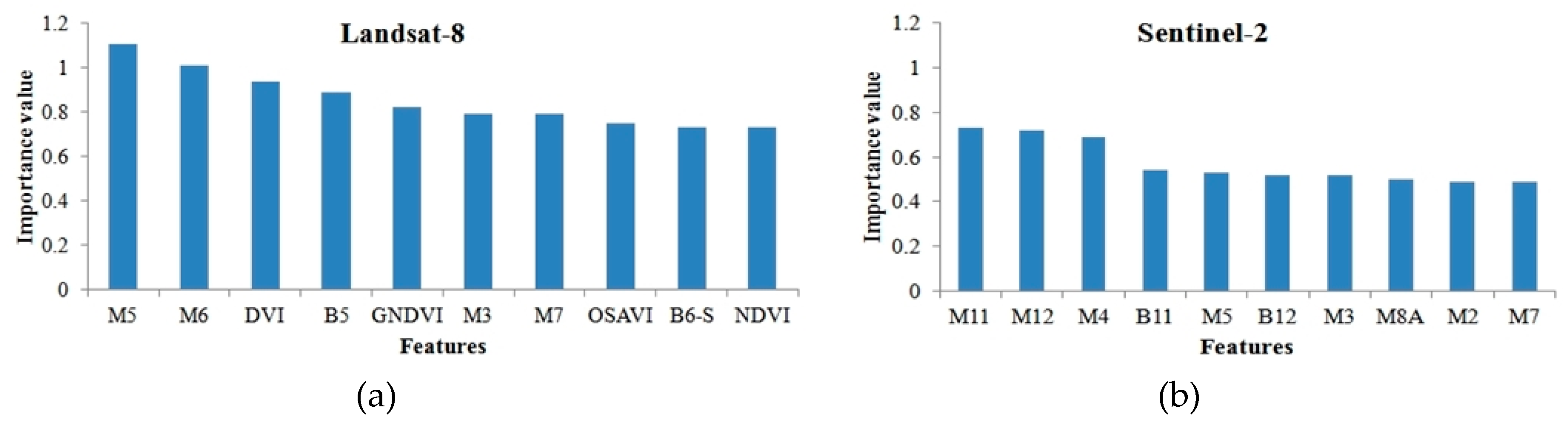
This study showed that the multispectral sensors Sentinel-2 and Landsat-8 are a valuable source of data for discriminating successional stages in an area of a subtropical forest. In the case of the Landsat-8 data, the addition of “spring” bands was more relevant to classification, considering the fact that three “spring” bands were chosen by the SVM classifier at the attributes selection stage (Table 5) and that one of them integrates the ranking of the 10 most important variables for the RF algorithm (Figure 6). One of the underlying reasons for this may be the solar geometry during image acquisition, since the “spring” scenes tend to present better illuminated pixels. Other authors also obtained better results when adding multitemporal information to their input dataset. Cetin et al. [83], when testing the efficacy of the contribution of Landsat-ETM+ and Terra ASTER multitemporal data for the semiautomatic classification of land cover and land use in Turkey, concluded that the combination of two multitemporal images resulted in slightly superior results. Murthy et al. [89] pointed out that the usage of multitemporal data increased the spectral separability of agricultural fields in India. Clark and Kilham [65] evaluated different metrics for classifying land cover and land use in California with HyspIRI simulated data and the RF classifier and they realized that the employment of multitemporal metrics increased the overall accuracy between 0.9% and 3.1% in comparison with the use of “Summer” metrics alone.

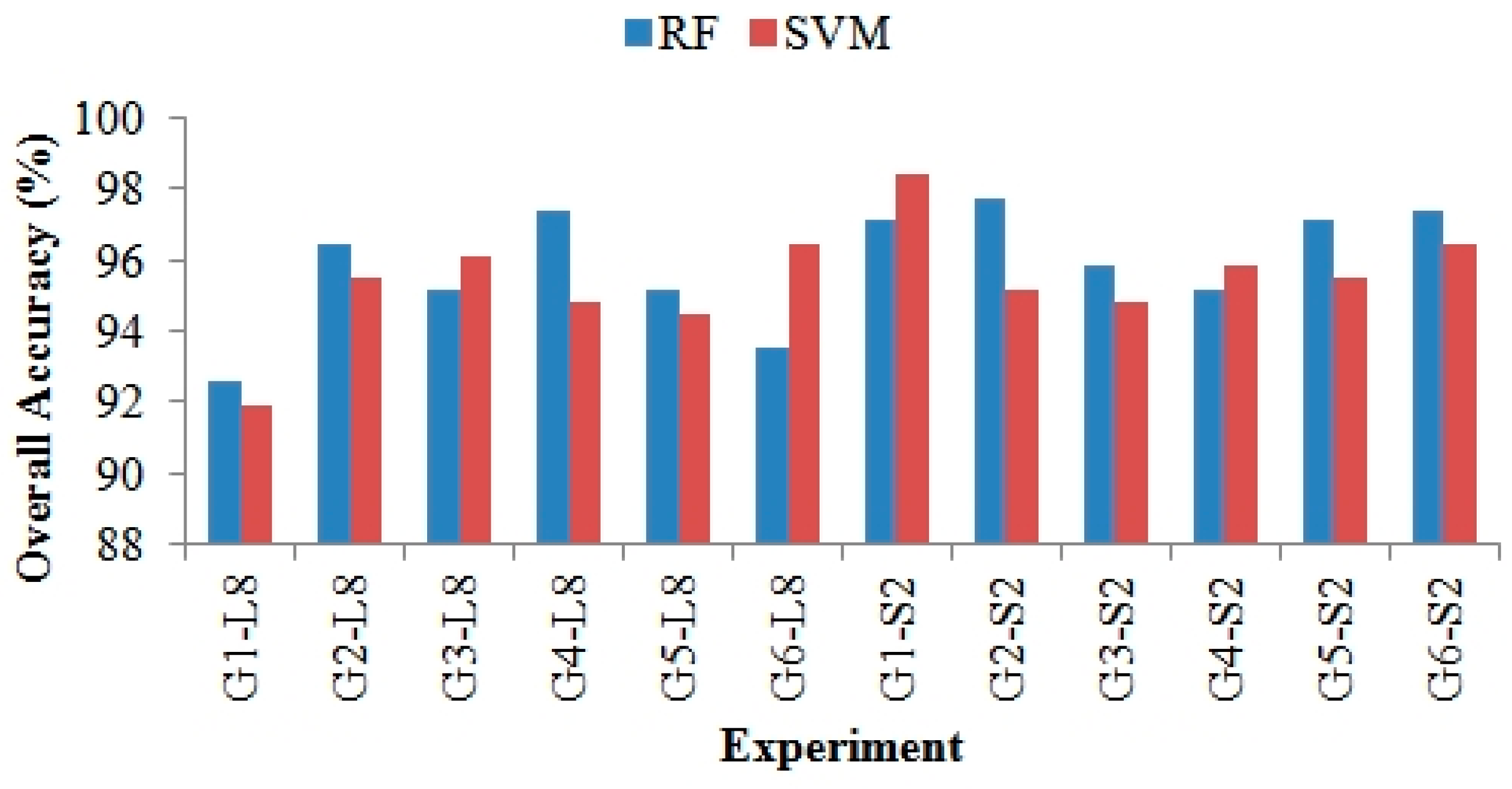
Regarding the classifiers performance, it was observed that the RF algorithm, when applied to the Sentinel-2 data, was less sensitive to the increase in variables when compared to SVM. In the experiment comprising all metrics (G5-S2), the SVM performance was significantly inferior in relation to using just the pure spectral bands of Sentinel-2, while, in the case of the RF classifier, the results of the G1-S2 and G5-S2 experiments did not present a significant difference. Walton [90] emphasizes the capacity of the RF algorithm in dealing with weak explanatory variables, which explains the fact that this was the only classifier that experienced increases in accuracy with the corresponding inclusion of variables in all evaluated experiments. Clark and Kilham [65] stress that one of the advantages of this classifier is its ability to handle well with predictor variables with multimodal distribution due to the high variability in time and space. This is the case of classes such as agricultural fields, which present variations in spectral response as a function of the type of culture and its life cycle, and forests, where the bidirectional reflectance factor varies according to the illumination conditions and their phenological properties. Novack et al. [91] also point out the fact that the RF classifier evaluates each attribute internally, and hence, it is less influenced by the correlation and dimensionality of the attributes hyperspace. As to the SVM, in the specific case of the G5-S2 experiment, the increase in the number of variables may have caused an overfit of the model to the training samples. However, this statement cannot be generalized, given that for the Landsat-8 data both classifiers improved their performance with the addition of new variables.

Regarding the employed multispectral data, both Landsat-8 and Sentinel-2 reached similar accuracies in most of the experiments. Nevertheless, when considering just the multispectral bands of each sensor, the Sentinel-2 data classification achieved a significantly superior accuracy to that obtained by the Landsat-8 data. This result agrees with the findings of Topaloglu et al. [92], who compared the performance of land cover and land use semiautomatic classification with the SVM and maximum likelihood algorithms and also using Sentinel-2 and Landsat-8 imagery. In that work, SVM presented a superior performance, with an overall accuracy of 81.7% for Landsat-8 data, and of 84.17% for Sentinel-2 data. Both classifiers attained a superior performance when dealing with Sentinel-2 data. Sothe et al. [93] comparatively evaluated the algorithms maximum likelihood and RF for classifying land cover and land use in a coastal environmental in the south of Brazil using Sentinel-2 and Landsat-8 imagery, and concluded as well that the classification with Sentinel-2 data obtained a superior performance to that executed with Landsat-8 data.

In the experiments accomplished with both satellites data, the texture mean was one of the most important variables for the two data sets, mainly Sentinel-2. The use of textural information was acknowledged as a strong attribute for differentiating vegetation classes by several authors [52,92,93,94,95,96,97]. Sette and Maillard [94] classified vegetation successional stages of a Dense Ombrophilous Forest in the Atlantic Rain Forest with FORMOSAT-2 imagery and obtained an overall accuracy of 60.5% based only on visible bands, which rose to 91% when the classification also relied on textural attributes. Araújo [95] verified an improvement in the discrimination between trees and grass with the introduction of an attribute indirectly based on texture, which considered the number of subobjects contained within each of these two classes in an immediately inferior segmentation level. According to the authors, since the texture of the trees class is rougher due to the presence of shadow amid the canopy leaves, this class tended to present a higher number of subobjects in comparison to grass.

Several authors highlighted the importance of both the SWIR and red-edge spectral regions for classifying forest types and agricultural fields [27,98,99]. Immitzer et al. [27], when using Sentinel-2 data for discriminating vegetation species and cultures with the RF classifier, also concluded that the SWIR and red-edge bands had a decisive importance in the images classification. Schultz et al. [98] used Landsat-8 data and RF for mapping cultures in the southeastern portion of Brazil, and they found that the SWIR-1 and SWIR-2 bands as well as NDVI were the most important predictor variables. Ramoelo et al. [99], when using Sentinel-2 data and the RF algorithm, verified that the SWIR-1 and SWIR-2 bands together with the first red-edge band achieved the highest importance values for assessing leaf nitrogen content in the African savannah. In many other works, the introduction of bands from the red-edge region in the classification process increased the separability among land cover and land use classes [11,100,101,102], and, hence, improved the classification accuracies of forests and agricultural fields.

Regarding the OLI sensor data, besides the SWIR bands texture means, the NIR band and three vegetation indices are worth mentioning, which stands in opposition to the MSI sensor, for which there was no vegetation index in the ranking of the most important variables. The listed vegetation indices (GNDVI, NDVI and OSAVI) explore the vegetation contrast between the NIR and visible bands, and might have been considered more relevant due to the fact that the OLI sensor does not provide data in the red-edge region. This can also be checked in the classification results, since according to Table 6, the inclusion of vegetation indices to the Sentinel-2 data set did not produce an increase in the classification accuracy, while for the Landsat-8 data, this led to a considerable improvement in the results. Satellites such as Sentinel-2 and Landsat-8 provide systematic coverage of the Earth surface, allowing a timely, cheap and large scale monitoring of forest remnants worldwide. This enables inspection and control of irregular activities (e.g., deforestation, illegal logging and forestry, etc.) as well as the conception of strategies for forest management and conservation. The information derived from these data can also support environmental regularization initiatives, such as the Rural Environmental Cadastre (CAR), a governmental program in Brazil designed for the inventory of natural assets and land cover/land use in rural properties.

5. Conclusions

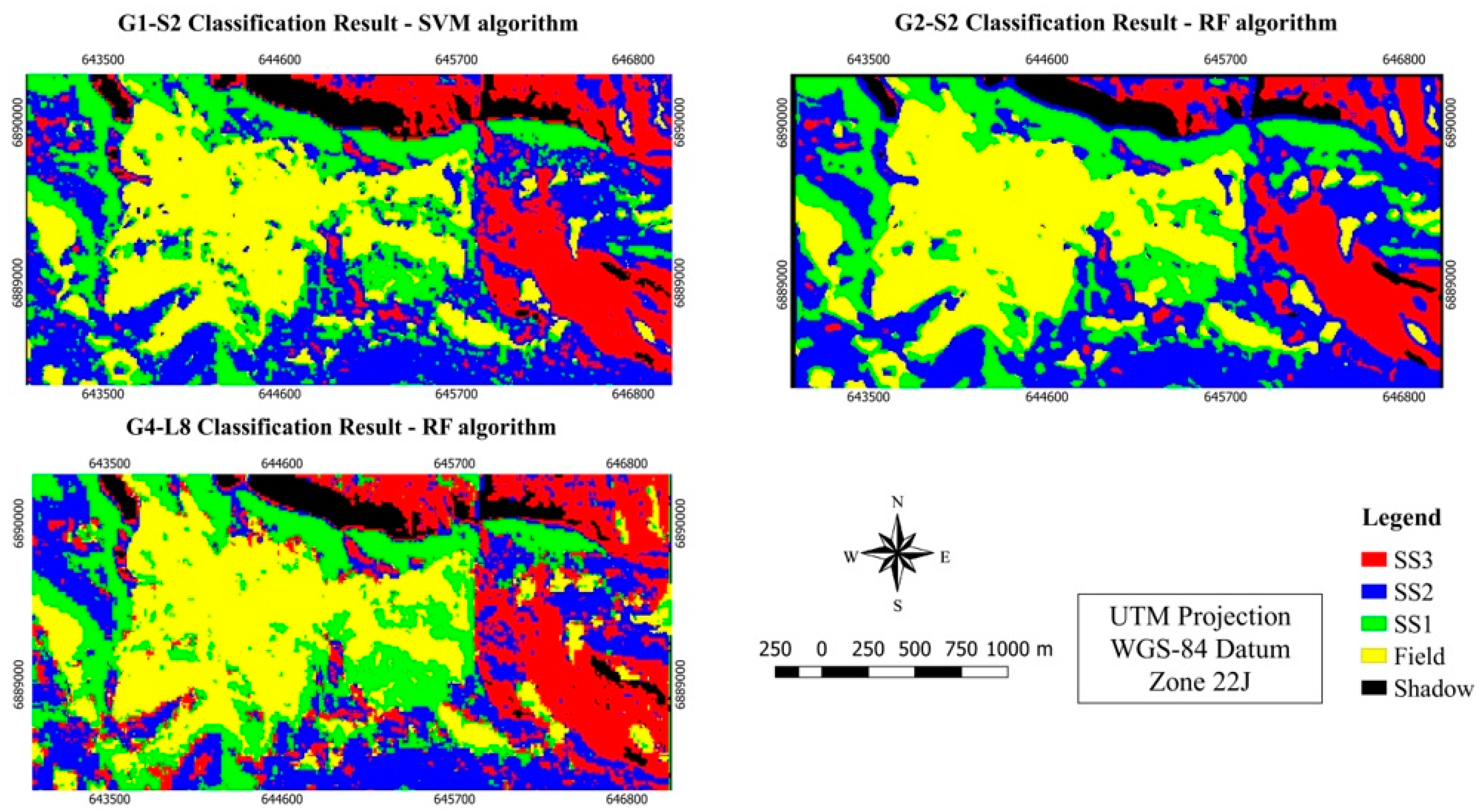
This study showed that both Landsat-8 and Sentinel-2 images have a great potential for the purpose of classifying vegetation successional stages in the study area. It is worth mentioning that the adopted methodology may be easily applied to further subtropical areas of the Atlantic Rain Forest with similar characteristics. The producer’s accuracy and user’s accuracy in all classification experiments were equal or superior to 80%. The best experiment attained a Kappa index of 0.98 (G1-S2 with SVM), while in the worst one this index reached 0.9 (G1-L8 with SVM), both comprising only the spectral bands of each sensor.

The addition of textural metrics, multitemporal information and vegetation indices in the classification process was important for increasing the accuracy of the Landsat-8 data classification, however, this did not bring meaningful improvements in the case of the Sentinel-2 images. For these latter data, the experiment that used spectral bands alone with the SVM classifier reached the highest accuracy, significantly superior to almost all of the experiments using Landsat-8 data. This fact can be explained by the greater spatial and spectral resolutions of MSI when compared to the OLI sensor.

The ranking with the 10 most important predictor variables showed that the texture means of SWIR and red-edge bands from both sensors as well as those derived from the Sentinel-2 red-edge bands are noteworthy, complying with other studies that also indicated that these spectral bands are of great relevance for the classification of vegetation. In face of the absence of red-edge spectral bands in the Landsat-8 satellite, the vegetation indices are instead present in such ranking of the most important variables.

With respect to the evaluated classifiers, it was observed that the RF showed to be less sensitive to the inclusion of variables in the classification process with the Sentinel-2 data, while the SVM classifier experienced a decrease in accuracy when using all variables. Nevertheless, this behavior was not observed for the Landsat-8 data, which in fact benefited from the inclusion of variables. As for the Landsat-8 data, the best result was achieved in the experiment that relied on multitemporal information, demonstrating that this sort of information should be explored with the intent of improving the classification accuracy of forest typologies.

Finally, this work indicated that the adopted approaches for the semiautomatic classification of the three successional stages in a patch of a subtropical portion of the Atlantic Rain Forest were promising. The herein produced findings are relevant not only for the conservation of this severely threatened biome, optimizing the mapping and monitoring of its forest remnants, but also for subsidizing actions in the scope of the Rural Environmental Cadastre (CAR) in Brazil, as exposed before. As directions for future work, we envisage expanding the study area and applying the tested methods in similar vegetation physiognomies.

References

1. Zhang, Z.; Zang, R.; Wang, G.; Huang, X. Classification of landscape types based on land cover, successional stages and plant functional groups in a species-rich forest in Hainan Island, China. Trop. Conserv. Sci. 2016, 9, 135–152. [Google Scholar] [CrossRef]
2. Viana, V.; Tabanez, A.J. Biology and Conservation of Forest Fragments in Brasilian Atlantic Moist Forest. In Forest Patches in Tropical Landscapes; Scheilas, J., Greenberg, R., Eds.; Island Press: Washington, DC, USA, 1996. [Google Scholar]
3. Ribeiro, M.C.; Metzger, J.P.; Martensen, A.C.; Ponzoni, F.J.; Hirota, M.M. The Brazilian Atlantic Forest: How much is left, and how is the remaining forest distributed? Implications for conservation. Biol. Conserv. 2009, 142, 1141–1153. [Google Scholar] [CrossRef]
4. Colombo, A.F.; Joly, C.A. Brazilian Atlantic Forest lato sensu: The most ancient Brazilian forest, and a biodiversity hotspot, is highly threatened by climate change. Braz. J. Biol. 2010, 70, 697–708. [Google Scholar] [CrossRef] [PubMed]
5. Myers, N.; Mittermeier, R.A.; Mittermeier, C.G.; Fonseca, G.A.B.; Kent, J. Biodiversity hotspots for conservation priorities. Nature 2000, 403, 853–858. [Google Scholar] [CrossRef] [PubMed]
6. Mausel, P.; Wu, Y.; Li, Y.; Moran, E.F.; Brondizio, E.S. Spectral identification of successional stages following deforestation in the Amazon. Geocarto Int. 1993, 8, 61–71. [Google Scholar] [CrossRef]
7. Lu, D.; Mausel, P.; Brondízio, E.; Moran, E. Classification of Successional Forest Stages in the Brazilian Amazon Basin. Forest Ecol. Manag. 2003, 181, 301–312. [Google Scholar] [CrossRef]
8. Lu, D.; Batistella, M.; Li, G.; Moran, E.; Hetrick, S.; Freitas, C.; Dutra, L.; Sant’Anna, S.J.S. Land use/Cover Classification in the Brazilian Amazon using Satellite Images. Braz. J. Agric. Res. 2012, 47, 1185–1208. [Google Scholar] [CrossRef] [PubMed]
9. Lu, D.; Li, G.; Moran, E.; Kuang, W. A comparative analysis of approaches for successional vegetation classification in the Brazilian Amazon. GISci. Remote Sens. 2014, 51, 695–709. [Google Scholar] [CrossRef]
10. Dispõe Sobre a Utilização e Proteção da Vegetação Nativa do Bioma Mata Atlântica, e dá Outras Providências. Available online: http://www2.ib.unicamp.br/profs/cjoly/0 - NE441 2013/2a AULA/Lei 11428 de 22-12-2006.pdf (accessed on 7 June 2017).
11. Adam, E.; Mutanga, O.; Odindi, J.; Abdel-Rahman, E.M. Land-use/cover classification in a heterogeneous coastal landscape using RapidEye imagery: Evaluating the performance of random forest and support vector machines classifiers. Int. J. Remote Sens. 2014, 35, 3440–3458. [Google Scholar] [CrossRef]
12. Janoth, J.; Eisl, M.; Klaushofer, F.; Luckel, W. Procedimentos Baseados em Segmentação para a Análise de Mudanças e Classificação Florestais com Dados de Satélite de Alta Resolução. In Sensoriamento Remoto e SIG Avançados, 2nd ed.; Blaschke, T., Kux, H., Eds.; Oficina de Textos: São Paulo, Brazil, 2007. [Google Scholar]
13. Vieira, I.C.G.; Almeida, A.S.; Davidson, E.A.; Stone, T.A.; Carvalho, C.J.R.; Guerrero, J.B. Classifying successional forests using Landsat spectral properties and ecological characteristics in Eastern Amazônia. Remote Sens. Environ. 2003, 87, 470–481. [Google Scholar] [CrossRef]
14. Ponzoni, F.J.; Rezende, A.N.P. Caracterização espectral de estágios sucessionais de vegetação secundária arbórea em Altamira (PA), através de dados orbitais. Rev. Árvore 2004, 28, 535–545. [Google Scholar] [CrossRef]
15. Galvão, L.S.; Ponzoni, F.J.; Liesenberg, V.; Santos, J.R.D. Possibilities of Discriminating Tropical Secondary Succession in Amazônia using Hyperspectral and Multiangular CHRIS/PROBA Data. Int. J. Appl. Earth Obs. Geoinf. 2009, 11, 8–14. [Google Scholar]
16. Amaral, M.V.F.; de Souza, A.L.; Soares, V.P.; Soares, C.P.B.; Leite, H.G.; Martins, S.V.; Filho, E.I.F.; Lana, J.M. Avaliação e comparação de métodos de classificação de imagens de satélites para o mapeamento de estádios de sucessão florestal. Rev. Árvore 2009, 33, 575–582. [Google Scholar] [CrossRef]
17. Li, G.; Lu, D.; Moran, E.; Hetrick, S. Land-Cover Classification in a Moist Tropical Region of Brazil with Landsat Thematic Mapper Imagery. Int. J. Remote Sens. 2011, 32, 8207–8230. [Google Scholar] [CrossRef] [PubMed]
18. Lu, D.; Li, G.; Moran, E.; Dutra, L.; Batistella, M. A Comparison of Multisensor Integration Methods for Land-cover Classification in the Brazilian Amazon. GISci. Remote Sens. 2011, 48, 345–370. [Google Scholar] [CrossRef]
19. Sothe, C.; Schimalski, M.B.; Liesenberg, V.; de Almeida, C.M.; de Souza, C.F.; de Souza, J.B. Applying data mining techniques to the classification of successional forest stages mixed shade tolerant forest environments. Sci. For. 2016, 44, 863–873. [Google Scholar]
20. Sothe, C.; Schimalski, M.B.; Liesenberg, V.; de Almeida, C.M. Approaches for classifying successional forest stages in São Joaquim National Park using Landsat-8 and RapidEye images. Bol. Ciênc. Geod. 2017, 23. in press. [Google Scholar]
21. Piazza, A.G.; Vibrans, A.C.; Liesenberg, V.; Refosco, J.C. Object-oriented and pixel-based classification approaches to classify tropical successional stages using airborne high–spatial resolution images. GISci. Remote Sens. 2016, 53, 206–226. [Google Scholar] [CrossRef]
22. Zhu, Z.; Woodcock, C.E. Continuous change detection and classification of land cover using all available Landsat data. Remote Sens. Environ. 2014, 144, 152–171. [Google Scholar] [CrossRef]
23. Roy, D.P.; Wulder, M.A.; Loveland, T.R.; Woodcock, C.E.; Allen, R.G.; Anderson, M.C.; Scambos, T.A. Landsat-8: Science and product vision for terrestrial global change research. Remote Sens. Environ. 2014, 145, 154–172. [Google Scholar] [CrossRef]
24. Irons, J.R.; Dwyer, J.L.; Barsi, J.A. The next Landsat satellite: The Landsat Data Continuity Mission. Remote Sens. Environ. 2012, 122, 11–21. [Google Scholar] [CrossRef]
25. Drusch, M.; Bello, U.D.; Carlier, S.; Colin, O.; Fernandez, V.; Gascon, F.; Hoersch, B.; Isola, C.; Laberinti, P.; Martimort, P.; et al. Sentinel-2: ESA’s Optical High-Resolution Mission for GMES Operational Services. Remote Sens. Environ. 2012, 120, 25–36. [Google Scholar] [CrossRef]
26. Frampton, W.J.; Dash, J.; Watmough, G.; Milton, E.J. Evaluating the capabilities of Sentinel-2 for quantitative estimation of biophysical variables in vegetation. ISPRS J. Photogramm. Remote Sens. 2013, 82, 83–92. [Google Scholar] [CrossRef]
27. Immitzer, M.; Vuolo, F.; Clement Atzberger, C. First Experience with Sentinel-2 Data for Crop and Tree Species Classifications in Central Europe. Remote Sens. 2016, 8, 166. [Google Scholar] [CrossRef]
28. Addabbo, P.; Focareta, M.; Marcuccio, S.; Votto, C.; Ullo, S.L. Contribution of Sentinel-2 data for applications in vegetation monitoring. Acta IMEKO 2016, 5, 44–54. [Google Scholar] [CrossRef]
29. Lu, D.; Weng, Q. A Survey of Image Classification Methods and Techniques for Improving Classification Performance. Int. J. Remote Sens. 2007, 28, 823–870. [Google Scholar] [CrossRef]
30. Deng, S.; Katoh, M.; Xiaowei, Y.; Hyyppä, J.; Gao, T. Comparison of Tree Species Classifications at the Individual Tree Level by Combining ALS Data and RGB Images Using Different Algorithms. Remote Sens. 2016. [Google Scholar] [CrossRef]
31. Prasad, A.M.; Iverson, L.R.; Liaw, A. Newer classification and regression tree techniques: Bagging and random forests for ecological prediction. Ecosystems 2006, 9, 181–199. [Google Scholar] [CrossRef]
32. Naidoo, L.; Cho, M.A.; Mathieu, R.; Asner, G. Classification of savanna tree species, in the Greater Kruger National Park region, by integrating hyperspectral and LiDAR data in a Random Forest data mining environment. ISPRS J. Photogramm. Remote Sens. 2012, 69, 167–179. [Google Scholar] [CrossRef]
33. Breiman, L. Random Forests. Mach. Learn. 2001, 45, 5–32. [Google Scholar] [CrossRef]
34. Li, M.; Ma, L.; Blaschke, T.; Cheng, L.; Tiede, D. A systematic comparison of different object-based classification techniques using high spatial resolution imagery in agricultural environments. Int. J. Appl. Earth Obs. Geoinf. 2016, 49, 87–98. [Google Scholar] [CrossRef]
35. Dalponte, M.; Bruzzone, L.; Gianelle, D. Tree species classification in the Southern Alps based on the fusion of very high geometrical resolution multispectral/hyperspectral images and LiDAR data. Remote Sens. Environ. 2012, 123, 258–270. [Google Scholar] [CrossRef]
36. Féret, J.; Asner, G.P. Tree species discrimination in tropical forests using airborne imaging spectroscopy. IEEE Trans. Geosci. Remote Sens. 2013, 51, 73–84. [Google Scholar] [CrossRef]
37. Gosh, A.; Fassnacht, E.F.; Joshi, P.K.; Koch, B. A framework for mapping tree species combining hyperspectral and LiDAR data: Role of selected classifiers and sensor across three spatial scales. Int. J. Appl. Earth Obs. Geoinf. 2014, 26, 49–63. [Google Scholar] [CrossRef]
38. Ma, L.; Li, M.; Ma, X.; Cheng, L.; Du, P.; Liu, Y. A review of supervised object-based land-cover image classification. ISPRS J. Photogramm. Remote Sens. 2017, 130, 277–293. [Google Scholar] [CrossRef]
39. Clark, M.L.; Roberts, D.A.; Clark, D.B. Hyperspectral discrimination of tropical rain forest tree species at leaf to crown scales. Remote Sens. Environ. 2005, 96, 375–398. [Google Scholar] [CrossRef]
40. Clark, M.L.; Roberts, D.A. Species-level differences in hyperspectral metrics among tropical rainforest trees as determined by a tree-based classifier. Remote Sens. 2012, 4, 1820–1855. [Google Scholar] [CrossRef]
41. Weih, R.C.; Riggan, N.D. Object-based Classification vs. Pixel-Based Classification: Comparative Importance of Multi-Resolution Imagery. Available online: http://dfwm.ugent.be/geobia/proceedings/papers%20proceedings/Weih_81_Object_Based_Classification_vs_Pixel_Based_Classification_Comparitive_Importance_of_Multi_Resolution_Imagery.pdf (accessed on 7 June 2017).
42. Meroni, M.; Ng, W-T.; Rembold, F.; Leonardi, U.; Atzberger, C.; Gadain, H.; Shaiy, M. Mapping prosopis juliflora in west somaliland with landsat 8 satellite imagery and ground information. Land Degrad. Dev. 2017, 28, 494–506. [Google Scholar] [CrossRef]
43. Faxina, T.C. Dilemas da regularização fundiária amigável no Parque Nacional de São Joaquim: Um estudo de caso—a valorização de áreas silvestres. Master’s Thesis, Santa Catarina State University, Lages-SC, Brazil, 2014. [Google Scholar]
44. Morellato, L.P.C.; Talora, D.C.; Takahasi, A.; Bencke, C.C.; Romera, E.C.; Zipparro, V.B. Phenology of Atlantic Rain Forest Trees: A Comparative Study. Blotroplca 2000, 32, 811–823. [Google Scholar] [CrossRef]
45. Marques, M.C.M.; Roper, J.J.; Salvalaggio, A.P.B. Phenological patterns among plant life-forms in a subtropical forest in southern Brazil. Plant Ecol. 2004, 173, 203–213. [Google Scholar] [CrossRef]
46. Song, C.; Woodcock, C.E. Monitoring forest succession with multitemporal Landsat images: Factors of uncertainty. IEEE Trans. Geosci. Remote Sens. 2003, 41, 2557–2567. [Google Scholar] [CrossRef]
47. Resolução CONAMA nº 04/94, de 4 de maio de 1994. Available online: http://www.mma.gov.br/port/conama/legiano1.cfm?codlegitipo=3&ano=1994 (accessed on 7 June 2017).
48. Soares, R.V. Considerações sobre a regeneração natural da Araucaria angustifolia. Rev. Floresta 1979, 10, 11–18. [Google Scholar] [CrossRef]
49. Haralick, R.M.; Shanmugam, K.; Dinstein, I.H. Textural features for image classification. IEEE Trans. Syst. Man Cybern. 1973, 3, 610–621. [Google Scholar] [CrossRef]
50. Marceau, D.J.; Howarth, P.J.; Dubois, J.M.; Gratton, D.J. Evaluation of the Grey-Level Co-occurrence Matrix Method for Land-cover Classification using SPOT Imagery. IEEE Trans. Geosci. Remote Sens. 1990, 28, 513–519. [Google Scholar] [CrossRef]
51. Johansen, K.; Coops, N.C.; Gergel, S.E.; Stange, Y. Application of High Spatial Resolution Satellite Imagery for Riparian and Forest Ecosystem Classification. Remote Sens. Environ. 2007, 110, 29–44. [Google Scholar] [CrossRef]
52. Yu, Q.; Gong, P.; Clinton, N.; Biging, G.; Kelly, M.; Schirokauer, D. Object-based Detailed Vegetation Classification with Airborne High Spatial Resolution Remote Sensing Imagery. Photogramm. Eng. Remote Sens. 2006, 72, 799–811. [Google Scholar] [CrossRef]
53. Furtado, L.F.A.; Francisco, C.N.; Almeida, C.M. Object-based image analysis for vegetation physiognomies classification in high spatial resolution images. Geociências 2013, 32, 441–451. [Google Scholar]
54. Lu, D.; Batistella, M. Exploring TM image texture and its relationships with biomass estimation in Rondônia, Brazilian Amazon. Acta Amazonica 2005, 35, 249–257. [Google Scholar] [CrossRef]
55. Attarchi, S.; Gloaguen, R. Classifying Complex Mountainous Forests with L-Band SAR and Landsat Data Integration: A Comparison among Different Machine Learning Methods in the Hyrcanian Forest. Remote Sens. 2014, 6, 3624–3647. [Google Scholar] [CrossRef]
56. Gitelson, A.A.; Merzlyak, M.N. Quantitative estimation of chlorophyll-a using reflectance spectra: Experiments with autumn chestnut and maple leaves. J. Photochem. Photobiol. B Biol. 1994, 22, 247–252. [Google Scholar] [CrossRef]
57. Hatfield, J.L.; Gitelson, A.A.; Schepers, J.S.; WalthalL, C.L. Application of Spectral Remote Sensing for Agronomic Decisions. Agron. J. 2008, 100, 117–131. [Google Scholar] [CrossRef]
58. Ji, L.; Zhang, L.; Wylie, B.K.; Rover, J. On the terminology of the spectral vegetation index (NIR − SWIR)/(NIR + SWIR). Int. J. Remote Sens. 2011, 32, 6901–6909. [Google Scholar] [CrossRef]
59. Rouse, J.W.; Haas, R.H.; Schell, J.A.; Deering, W.D. Monitoring vegetation systems in the Great Plains with ERTS. Third ERTS Sym. NASA SP-351 1973, 1, 309–317. [Google Scholar]
60. Richardson, A.J.; Wiegand, C.L. Distinguishing vegetation from soil background information. Photogramm. Eng. Remote Sens. 1977, 1, 1541–1552. [Google Scholar]
61. Gitelson, A.A.; Kaufman, Y.J.; Merzlyak, M.N. Use of a green channel in remote sensing of global vegetation from EOS-MODIS. Remote Sens. Environ. 1996, 58, 289–298. [Google Scholar] [CrossRef]
62. Tucker, C.J. Red and photographic infrared linear combinations for monitoring vegetation. Remote Sens. Environ. 1979, 8, 127–150. [Google Scholar] [CrossRef]
63. Rondeaux, G.; Steven, M.; Baret, F. Optimization of soil-adjusted vegetation indices. Remote Sens. Environ. 1996, 55, 95–107. [Google Scholar] [CrossRef]
64. Hardisky, M.A.; Klemas, V.; Smart, R.M. The influence of soil salinity, growth form, and leaf moisture on the spectral radiance of Spartina alterniflora canopies. Photogramm. Eng. Remote Sens. 1983, 49, 77–83. [Google Scholar]
65. Clark, M.L.; Kilham, N.E. Mapping of land cover in northern California with simulated hyperspectral satellite imagery. ISPRS J. Photogramm. Rem. Sens. 2016, 119, 228–245. [Google Scholar] [CrossRef]
66. Pal, M.; Foody, G.M.P. Feature Selection for Classification of Hyperspectral Data by SVM. IEEE Trans. Geosci. Remote Sens. 2010, 48, 2297–2307. [Google Scholar] [CrossRef]
67. Ma, L.; Fu, T.; Blaschke, T.; Li, M.; Tiede, D.; Zhou, Z.; Chen, D. Evaluation of Feature Selection Methods for Object-Based Land Cover Mapping of Unmanned Aerial Vehicle Imagery Using Random Forest and Support Vector Machine Classifiers. ISPRS Int. J. Geo-Inf. 2017, 6, 51. [Google Scholar] [CrossRef]
68. Duro, D.C.; Franklin, S.E.; Dubé, M.G. Multi-scale object-based image analysis and feature selection of multi-sensor earth observation imagery using random forests. Int. J. Remote Sens. 2012, 33, 4502–4526. [Google Scholar] [CrossRef]
69. Hira, Z.M.; Gillies, D.F. A Review of Feature Selection and Feature Extraction Methods Applied on Microarray Data. Adv. Bioinf. 2015. [Google Scholar] [CrossRef] [PubMed]
70. Maldonado, S.; Weber, R. A wrapper method for feature selection using support vector machines. Inf. Sci. 2009, 179, 2208–2217. [Google Scholar] [CrossRef]
71. Puissant, A.; Rougier, S.; Stumpf, A. Object-oriented mapping of urban trees using random forest classifiers. Int. J. Appl. Earth Obs. Geoinf. 2014, 26, 235–245. [Google Scholar] [CrossRef]
72. Ma, L.; Li, M.; Gao, Y.; Chen, T.; Ma, X.; Qu, L. A Novel Wrapper Approach for Feature Selection in Object-Based Image Classification Using Polygon-Based Cross-Validation. IEEE Geosci. Remote Sens. Lett. 2017, 14, 409–413. [Google Scholar] [CrossRef]
73. Kohavi, R.; John, G.H. Wrappers for feature subset selection. Artif. Intell. 1997, 97, 273–324. [Google Scholar] [CrossRef]
74. Van der Linden, S.; Rabe, A.; Held, M.; Wirth, F.; Suess, S.; Okujeni, A.; Hostert, P. ImageSVM Classification, Manual for Application: ImageSVM Version 3.0; Humboldt-Universität: Berlin, Germany, 2014. [Google Scholar]
75. Van der Linden, S.; Rabe, A.; Held, M.; Jakimow, B.; Leitão, P.J.; Okujeni, A.; Schwieder, S.S.; Hostert, P. The EnMAP-Box—A Toolbox and Application Programming Interface for EnMAP Data Processing. Remote Sens. 2015, 7, 11249–11266. [Google Scholar] [CrossRef]
76. Rodriguez-Galiano, V.F.; Ghimire, B.; Rogan, J.; Chica-Olmo, M.; Rigol-Sanchez, J.P. An assessment of the effectiveness of a random forest classifier for landcover classification. ISPRS J. Photogramm. Rem. Sens. 2012, 67, 93–104. [Google Scholar] [CrossRef]
77. Jakimow, B.; Oldenburg, C.; Rabe, A.; Waske, B.; van der Linden, S.; Hostert, P. ImageRF Classification, Manual for Application: ImageRF Version 1.1; Humboldt-Universität: Berlin, Germany, 2014. [Google Scholar]
78. Cortes, C.; Vapnik, V. Support-Vector Networks. Mach. Learn. 1995, 20, 273–297. [Google Scholar] [CrossRef]
79. Huang, C.; Davis, L.S.; Townshend, J.R.G. An assessment of support vector machines for land cover classification. Remote Sens. 2002, 23, 725–749. [Google Scholar] [CrossRef]
80. Duro, D.C.; Franklin, S.E.; Dube, M.G. A comparison of pixel-based and object-based image analysis with selected machine learning algorithms for the classification of agricultural landscapes using SPOT-5 HRG imagery. Remote Sens. Environ. 2012, 118, 259–272. [Google Scholar] [CrossRef]
81. Burges, C.J. A tutorial on support vector machines for pattern recognition. Data Min. Knowl. Discov. 1998, 2, 121–167. [Google Scholar] [CrossRef]
82. Li, W.; Du, Q. Support vector machine with adaptive composite kernel for hyperspectral image classification. Proc. SPIE. [CrossRef]
83. Congalton, R.G.; Green, K. Assessing the Accuracy of Remotely Sensed Data: Principles and Practices; Lewis Publishers: New York, NY, USA, 1999. [Google Scholar]
84. Skidmore, A.K. Accuracy Assessment of Spatial Information. In Spatial Statistics for Remote Sensing; Stein, A., van der Meer, F.D., Gorte, B., Eds.; Kluwer Academic Publishers: Dordrecht, The Netherlands, 1999; pp. 197–209. [Google Scholar]
85. Cetin, M.; Kavzoglu, T.; Musaoglu, N. Classification of multi-spectral, multi-temporal and multi-sensor images using principal components analysis and artificial neural networks: Beykoz case. In Proceedings of the XXXV ISPRS Congress, Melbourne, Australia, 25 August–1 September 2012; p. 408. [Google Scholar]
86. Moran, E.F.; Brondizio, E.S.; Tucker, J.M.; Silva-Fosberg, M.C.; McCracken, S.; Falesi, I. Effects of soil fertility and land-use on forest successional in Amazônia. Forest Ecol. Manag. 2000, 139, 93–108. [Google Scholar] [CrossRef]
87. Ponzoni, F.J.; Shimabukuro, Y.E.; Kuplich, T.M. Sensoriamento Remoto da Vegetação; Oficina de Textos: São Paulo, Brazil, 2012. [Google Scholar]
88. Goel, N.S. Models of vegetation canopy reflectance and their use in estimation of biophysical parameters from reflectance data. Remote Sens. Rev. 1988, 4, 1–21. [Google Scholar] [CrossRef]
89. Murthy, C.S.; Raju, P.V.; Badrinath, K.V.S. Classification of wheat crop with multi-temporal images: Performance of maximum likelihood and artificial neural networks. Int. J. Remote Sens. 2003, 24, 4871–4890. [Google Scholar] [CrossRef]
90. Walton, J.T. Subpixel Urban Land Cover Estimation: Comparing Cubist, Random Forests, and Support Vector Regression. Photogramm. Eng. Remote Sens. 2008, 74, 1213–1222. [Google Scholar] [CrossRef]
91. Novack, T.; Esch, T.; Kux, H.; Stilla, U. Machine Learning Comparison between WorldView-2 and QuickBird-2-Simulated Imagery Regarding Object-Based Urban Land Cover Classification. Remote Sens. 2011, 3, 2263–2282. [Google Scholar] [CrossRef]
92. Topaloglu, R.H.; Sertela, E.; Musaoglu, N. Assessment of classification accuracies of Sentinel-2 and Landsat-8 data for land cover/use mapping. In Proceedings of the International Archives of the Photogrammetry, Remote Sensing and Spatial Information Sciences, 41-B8, XXIII ISPRS Congress, Prague, Czech Republic, 12–19 July 2016; pp. 1055–1059. [Google Scholar]
93. Sothe, C.; Schimalski, M.B.; Liesenberg, V.; de Almeida, C.M. Potencial dos dados Sentinel-2 e Landsat-8 para a classificação do uso e cobertura da terra de um ambiente costeiro. In Proceedings of the XVIII Brazilian Symposium on Remote Sensing—SBSR, Santos, SP, Brazil, 28–31 May 2017. [Google Scholar]
94. Sette, P.G.C.; Maillard, P. Análise de textura de imagem de alta resolução para aprimorar a acurácia da classificação da mata atlântica no sul da Bahia. In Proceedings of the XV Brazilian Symposium on Remote Sensing-SBSR, Curitiba, PR, Brazil, 29 April–4 May 2011. [Google Scholar]
95. Araújo, E.H.G. Análise Multi-Temporal de Cenas do Satélite QuickBird Usando um novo Paradigma de Classificação de Imagens e Inferências Espaciais. Estudo de Caso: Belo Horizonte, MG. (INPE-13956-TDI/1062). Master’s Thesis, National Institute for Space Research, São José dos Campos, 2006. [Google Scholar]
96. Roslani, M.A.; Mustapha, M.A.; Lihan, T.; Wan Juliana, W.A. Classification of mangroves vegetation species using texture analysis on Rapideye satellite imagery. AIP Conf. Proc. 2013, 1571, 480. [Google Scholar]
97. Gomes, M.F.; Maillard, P. Using spectral and textural features from RapidEye images to estimate age and structural parameters of Cerrado vegetation. Int. J. Remote Sens. 2015, 36, 3058–3076. [Google Scholar] [CrossRef]
98. Schultz, B.; Immitzer, M.; Formaggio, A.R.; Sanches, I.D.A.; Luiz, A.J.B.; Atzberger, C. Self-Guided Segmentation and Classification of Multi-Temporal Landsat 8 Images for Crop Type Mapping in Southeastern Brazil. Remote Sens. 2015, 7, 14482–14508. [Google Scholar] [CrossRef]
99. Ramoelo, A.; Cho, M.; Mathieu, R.; Skidmore, A.K. Potential of Sentinel-2 spectral configuration to assess rangeland quality. J. Appl. Remote Sens. 2015. [Google Scholar] [CrossRef]
100. Schuster, C.; Förster, M.; Kleinschmit, B. Testing the Red Edge Channel for Improving Land-Use Classifications Based on High-Resolution Multi-Spectral Satellite Data. Int. J. Remote Sens. 2012, 33, 5583–5599. [Google Scholar] [CrossRef]
101. Tigges, J.; Lakes, T.; Hostert, P. Urban vegetation classification: Benefits of multitemporal RapidEye satellite data. Remote Sens. Environ. 2013, 136, 66–75. [Google Scholar] [CrossRef]
102. Adelabu, S.; Mutanga, O.; Adam, E. Evaluating the impact of red-edge band from Rapideye image for classifying insect defoliation levels. ISPRS J. Photogramm. Remote Sens. 2014, 95, 34–41. [Google Scholar] [CrossRef]
Figure 1. Methodological framework developed in this study.
Remotesensing 09 00838 g001
Figure 2. Study area location: (a) Santa Catarina State; (b) São Joaquim National Park; and (c) Study area over a Sentinel-2/MSI true color composition image.
Remotesensing 09 00838 g002
Figure 3. Vegetation successional stages relating the reference multispectral data (Orthoimage) and the employed orbital images (Sentinel-2 and Landsat-8) in true color composition.
Remotesensing 09 00838 g003
Figure 4. Example of pixel random sampling for accuracy assessment.
Remotesensing 09 00838 g004
Figure 5. (a,b) Spectral reflectance curves of the vegetation successional stages for the multispectral bands of Landsat-8/OLI and Sentinel-2/MSI sensors, fall season.
Remotesensing 09 00838 g005
Figure 6. (a,b) Ranking showing the 10 most important variables (features) for the RF classification. M, texture mean; B, spectral band; B-S, spectral band of the “spring” scene. See Table 3 and Table 4 for a complete description of variables.
Remotesensing 09 00838 g006
Figure 7. Overall Accuracy (OA) for all classification experiments.
Remotesensing 09 00838 g007
Figure 8. Best classification results obtained by Sentinel-2 and Landsat-8 data.
Remotesensing 09 00838 g008