
A Global Analysis of Sentinel-2A, Sentinel-2B and Landsat-8 Data Revisit Intervals and Implications for Terrestrial Monitoring


Geospatial Sciences Center of Excellence, South Dakota State University, Brookings, SD 57007, USA
*
Author to whom correspondence should be addressed.
Remote Sens. 2017, 9(9), 902; https://doi.org/10.3390/rs9090902
Submission received: 29 July 2017
/
Revised: 22 August 2017
/
Accepted: 22 August 2017
/
Published: 31 August 2017
(This article belongs to the Section Remote Sensing in Agriculture and Vegetation)
Abstract
:Combination of different satellite data will provide increased opportunities for more frequent cloud-free surface observations due to variable cloud cover at the different satellite overpass times and dates. Satellite data from the polar-orbiting Landsat-8 (launched 2013), Sentinel-2A (launched 2015) and Sentinel-2B (launched 2017) sensors offer 10 m to 30 m multi-spectral global coverage. Together, they advance the virtual constellation paradigm for mid-resolution land imaging. In this study, a global analysis of Landsat-8, Sentinel-2A and Sentinel-2B metadata obtained from the committee on Earth Observation Satellite (CEOS) Visualization Environment (COVE) tool for 2016 is presented. A global equal area projection grid defined every 0.05° is used considering each sensor and combined together. Histograms, maps and global summary statistics of the temporal revisit intervals (minimum, mean, and maximum) and the number of observations are reported. The temporal observation frequency improvements afforded by sensor combination are shown to be significant. In particular, considering Landsat-8, Sentinel-2A, and Sentinel-2B together will provide a global median average revisit interval of 2.9 days, and, over a year, a global median minimum revisit interval of 14 min (±1 min) and maximum revisit interval of 7.0 days.

1. Introduction
It is well established that combination of different optical wavelength satellite data provide increased opportunities for cloud-free surface observation [1,2,3,4]. The recent availability of near-contemporaneous Landsat-8 and Sentinel-2 data will provide increased opportunities at medium resolution [5,6], especially after the successful launch of Sentinel-2B in 2017 that now provide, with Sentinel-2A and Landsat-8, three medium resolution sun synchronous satellites on orbit. When remote sensing satellite orbits are designed, the satellite coverage may be considered in several ways including the number of observations in a given period and the revisit interval [7,8,9]. Previously, researchers have examined the number of observations in different periods for Landsat [10,11,12,13] and Sentinel-2 [14]. However, the revisit interval, i.e., the time period between consecutive observations of a surface location, has not been studied but is of considerable interest for terrestrial applications. In particular, change detection requires image acquisition before and after the change or disturbance event, with an appropriate observation frequency depending on the degree and persistence of the change compared to phenological and other temporal surface variations [15,16,17,18]. Near coincident observations are also useful for sensor comparison and characterization purposes, as they do not require the application of filters to remove residual surface and atmospheric changes. Landsat and Sentinel-2A data have been shown to provide near-coincident observations less than 20 min apart [19,20] but no global analysis of this has been undertaken.
In this paper, the total number of observations and the minimum, mean, and maximum revisit intervals for different combinations of Landsat-8, Sentinel-2A, and Sentinel-2B data are quantified. This is undertaken globally for one year using the committee on Earth Observation Satellite (CEOS) Visualization Environment (COVE) tool [21] without considering cloud cover as the Sentinel-2A and -2B satellites are only just producing global coverage data and the cloud mask product is still being refined. The results are reported using a global equal area projection, rather than a latitude–longitude grid, to provide unbiased global summary statistics.
2. Satellite Sensors and Orbits
2.1. Satellite Remote Sensing Configurations
Landsat-8 was launched on 11 February 2013 and carries the Operational Land Imager (OLI) and the Thermal Infrared Sensor (TIRS) in a circular sun-synchronous orbit with an altitude and inclination of approximately 705 km and 98.22°, respectively, and an equatorial crossing time of 10:00 a.m. ± 15 min [22]. The data are acquired with a 15° field of view providing an approximately 185 km swath, and the equatorial repeat cycle is 16 days. Sentinel-2 carries the Multi Spectral Instrument (MSI) [5]. Sentinel-2A was launched on 23 June 2015 and Sentinel-2B was launched 7 March 2017 into circular sun-synchronous 786 km orbits with 98.62° inclination and equatorial crossing times of 10:30 a.m. and with a phase delay of 180° [23]. The data are acquired with a 20.6° field of view providing an approximately 290 km swath, and the equatorial repeat cycle of each Sentinel-2 sensor is 10 days, and five days when combined.
2.2. Sensor Orbit Swath Simulation with the CEOS Visualization Environment (COVE) Tool
The orbit swaths and overpass times of Landsat-8, Sentinel-2A and Sentinel-2B were derived globally for 1 January to 31 December 2016 using the committee on Earth Observation Satellite (CEOS) Visualization Environment (COVE) tool [21]. Recently, the COVE tool was used by Whitcraft et al. [14] to simulate the number of observations provided by different combinations of medium resolution satellites (Landsat-7, Landsat-8, Sentinel-2A, Sentinel-2B, and Resourcesat-2) with respect to agricultural applications, from 60°N to 60°S, and for periods up to 180 days. The COVE tool models the orbits and coincident overpasses of multiple satellite missions using orbit and sensor models and satellite ephemeras information. For current or past missions the COVE tool uses a Simplified General Perturbation 4 (SGP4) propagator with satellite position and velocity data, and two-line elements (TLE), to predict the satellite orbit [21]. The orbit swaths can be visualized via an Internet browser, and, as in this study, can be downloaded as KML files truncated along-track into one-minute granules. At the equator, the KML granules cover about 412 km and 404 km in the track direction for Landsat-8 and Sentinel-2A/-2B, respectively. A total of 274,857, 274,797, and 273,782 one-minute granules for Sentinel-2A, Sentinel-2B, and Landsat-8 were downloaded for 2016, respectively. Only the daytime swaths were considered (defined as granules acquired with solar zenith angle <90°). Each KML file includes the acquisition date and time and the corner latitude and longitude defined in degrees to three decimal places (d.p.).
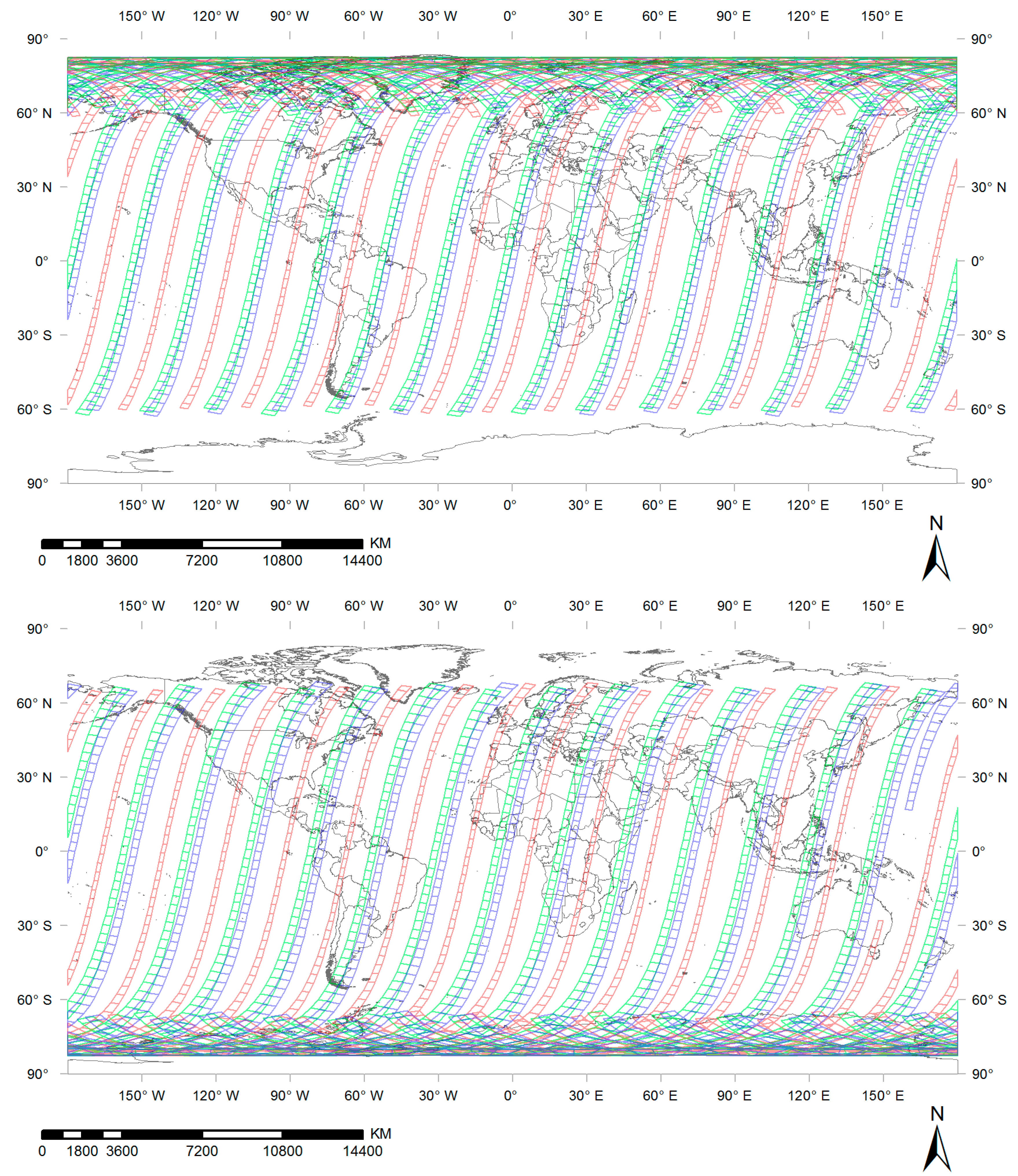
Figure 1 illustrates COVE Sentinel-2A, Sentinel-2B and Landsat-8 one minute granules for the summer solstice, 21 June 2016 (top), and the winter solstice, 21 December 2016 (bottom), defined in the geographic projection. The satellite tracks reflect their polar sun-synchronous orbits. It is evident that the orbit swath increases further polewards (due to the convergence of lines of longitude at higher latitude). The Landsat-8 swath is narrower (185 km) than for Sentinel-2 (290 km) due to the smaller field of view and lower orbit. The three sensor swaths overlap laterally with increasing overlap further polewards. There are no data at latitudes above approximately latitude 62.1°S and 67.7°N on the summer and winter solstices, respectively, because the satellites overpass in darkness (solar zenith angle ≥ 90°).
3. Methodology
The total number of observations and revisit interval metrics considering different combinations of Landsat-8, Sentinel-2A and Sentinel-2B data were examined with respect to a global grid. The grid was composed of 7201 × 3601 points spaced every 5.559752 km, equivalent to 0.05° at the Equator, defined in the uninterrupted equal area sinusoidal projection [4]. An equal area projection is needed so that area summary statistics are unbiased over different geographic units [24]. Using a regular grid of points in the geographic projection is inappropriate because the surface area sensed by each sensor is not sampled with the same spatial grid density further poleward [4].
A spatial sorting algorithm was implemented to obtain the KML granules of each sensor and sensor combination encompassing each global grid point over the year. This was undertaken by considering each global grid point independently and searching through all the KML granules considering their corner coordinates with respect to each grid point. A pre-sort algorithm was applied to filter out KML granules with center coordinates falling further away than several degrees of each grid point. Then a standard point in polygon routine [25] was applied to establish which granules encompassed each grid point. The total number of sensor observations of each grid point in 2016 was found by counting. If there was no observation of a grid point then a unique fill value was assigned.
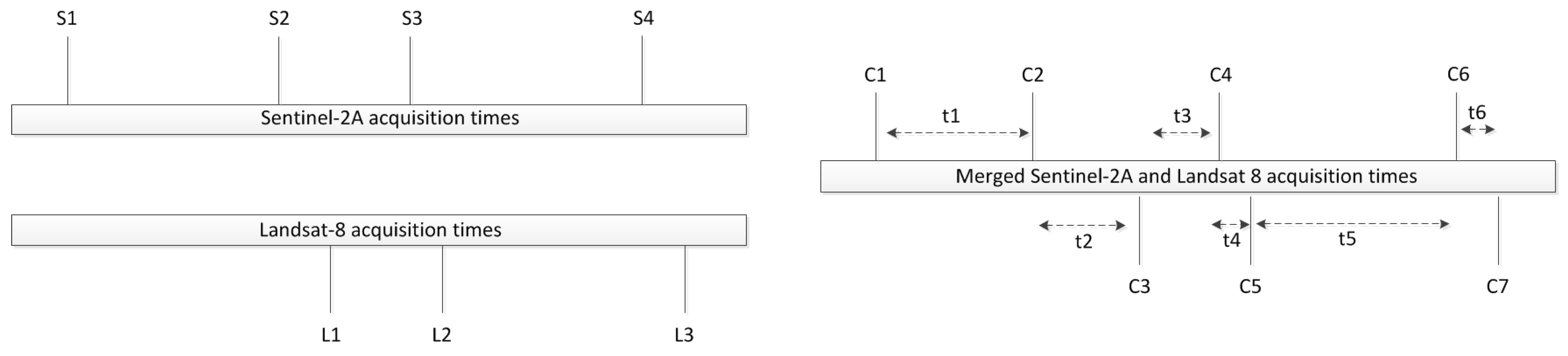
The revisit interval between successive observations of each grid point required the implementation of a temporal sorting algorithm. This is complicated because on the same day different sensors may overlap laterally and the order that a particular sensor first overpasses is unknown (Figure 1). Figure 2 illustrates the temporal sorting algorithm, showing the acquisition date/times of example Sentinel-2A and Landsat-8 granules encompassing the same grid point. First, the date and time of each sensor were chronologically ordered independently, e.g., the Sentinel-2A observations were sensed on S1, S2, S3, and S4, and the Landsat-8 observations were sensed on L1, L2, and L3. Then, the sorted set of date/times for each sensor were merged and sorted into a single combined set C that preserves the temporal order. Given the large amount of data, a computationally efficient sort algorithm was used [26]. The revisit intervals between successive sensors, e.g., t1, t2, t3, t4, t5, and t6, were derived from the single combined set.
The revisit interval results were rounded to the nearest minute, as each COVE KML granule corresponds to one minute in the track direction (Figure 1). For each grid location, the minimum, mean and maximum revisit intervals over the year were calculated. Summary global statistics, histograms, and maps, of the total number of observations and of the minimum, mean and maximum revisit intervals were derived.
4. Results
4.1. Annual Number of Observations
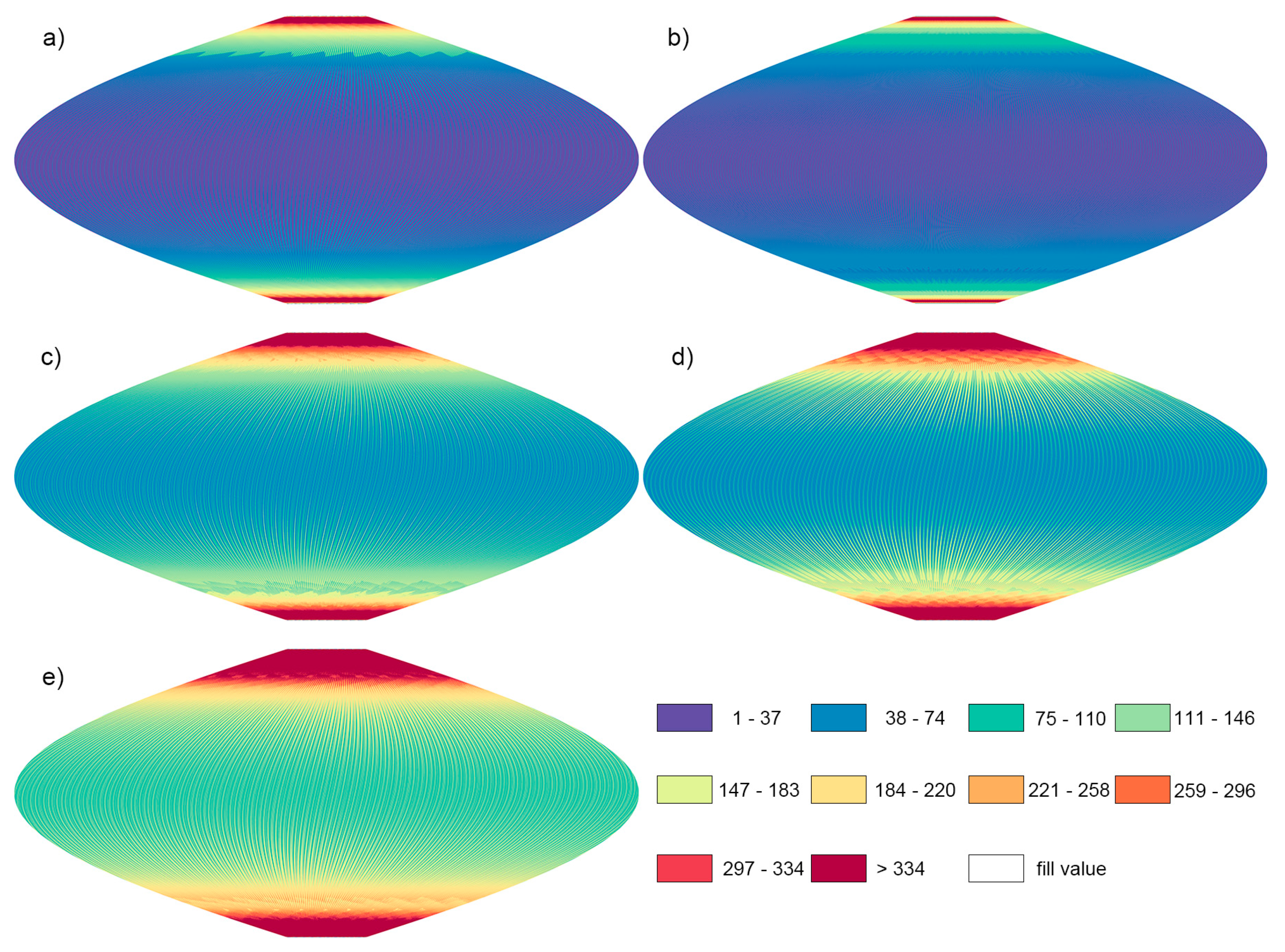
Figure 3 shows the total number of observations sensed over each global grid point in 2016 for Sentinel-2A (Figure 3a), Landsat-8 (Figure 3b), Sentinel-2A and Landsat-8 (Figure 3c), Sentinel-2A and Sentinel-2B (Figure 3d), and all three sensors (Figure 3e). Where there were no observations, the grid locations are colored white. The greater availability of Sentinel-2A data (Figure 3a) compared to Landsat-8 (Figure 3b), particularly at high latitudes, is evident and is due to the wider Sentinel-2 swath width and smaller repeat cycle. As expected, combining more satellites provides a greater number of annual observations and there are a greater number of observations further polewards. At latitudes above about 60° the annual number of observations increases rapidly to more than once per day, and more than four per day at the highest latitudes, when all three sensors are combined. Due to the retrograde inclination of the satellite orbits, the maximum northerly latitude that intersected a 0.05° global grid point is 82.8°N (Sentinel-2A) and 82.7°N (Landsat-8) and the most southerly latitude is 82.8°S (Sentinel-2A) and 82.7°S (Landsat-8). The results for Sentinel-2B, and, for both Sentinel-2B and Landsat-8, are not illustrated as they are very similar to the illustrated Sentinel-2A (Figure 3a) and the Sentinel-2A and Landsat-8 (Figure 3d) results, respectively.
Figure 4 shows histograms of the Figure 3 results. The different global histograms are positively skewed (a greater frequency of small values) and do not have uniform distributions. This is due to the lateral overlap of the orbits and the convergence of the orbits further polewards (Figure 1). Consequently, parametric summary statistics, such as the global mean or standard deviation values, are not particularly representative. This is evident in Table 1 that summarizes the global mean, median, and the first, second and third most frequent number of observations for each of the different sensor combinations. The global mean values are always greater than the median values due to the positively skewed histogram distributions. For each sensor alone, the global median annual number of observations corresponds closely to the number of days in the year divided by the sensor repeat cycle (i.e., 23, 37 and 37 for Landsat-8, Sentinel-2A and Sentinel-2B, respectively). When sensors are combined, the overlap of the different sensor orbits increase the median values considerably to 81 for Landsat-8 and either Sentinel-2 sensor, to 100 for both Sentinel-2 sensors, and to 127 for all three sensors. There are small differences between the Sentinel-2A and Sentinel-2B summary statistics. This is not an error but reflects the different dates of the first Sentinel-2A and Sentinel-2B January overpasses and the 10-day Sentinel-2 repeat cycle means that the two sensors have a slightly different number of overpasses over the 366 days of 2016.
The most frequent annual number of observations is the same as the median number for the single sensors and occurs for 47.9%, 35.9% and 36.3% of the globe for Landsat-8, Sentinel-2A and Sentinel-2B respectively. For combined sensors, there are more complex patterns, evident in Figure 3c–e and Figure 4c–e, and the most frequent annual number of observations is smaller than the median values (Table 1). When all three sensors are considered, there is a great diversity geographically in the number of annual observations; the first, second and third most frequent number of annual observations is 96, 133, and 118 and occurs for 21.1%, 9.6% and 0.1% of the globe; i.e., about 69% of the globe has a different number of annual observations. A similar diversity of values is found considering Landsat-8 and one Sentinel-2 satellite. When both Sentinel-2 satellites are considered together, about 52% of the globe has a different number of annual observations to the top three most frequent ones tabulated in Table 1.
4.2. Average Revisit Intervals
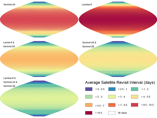
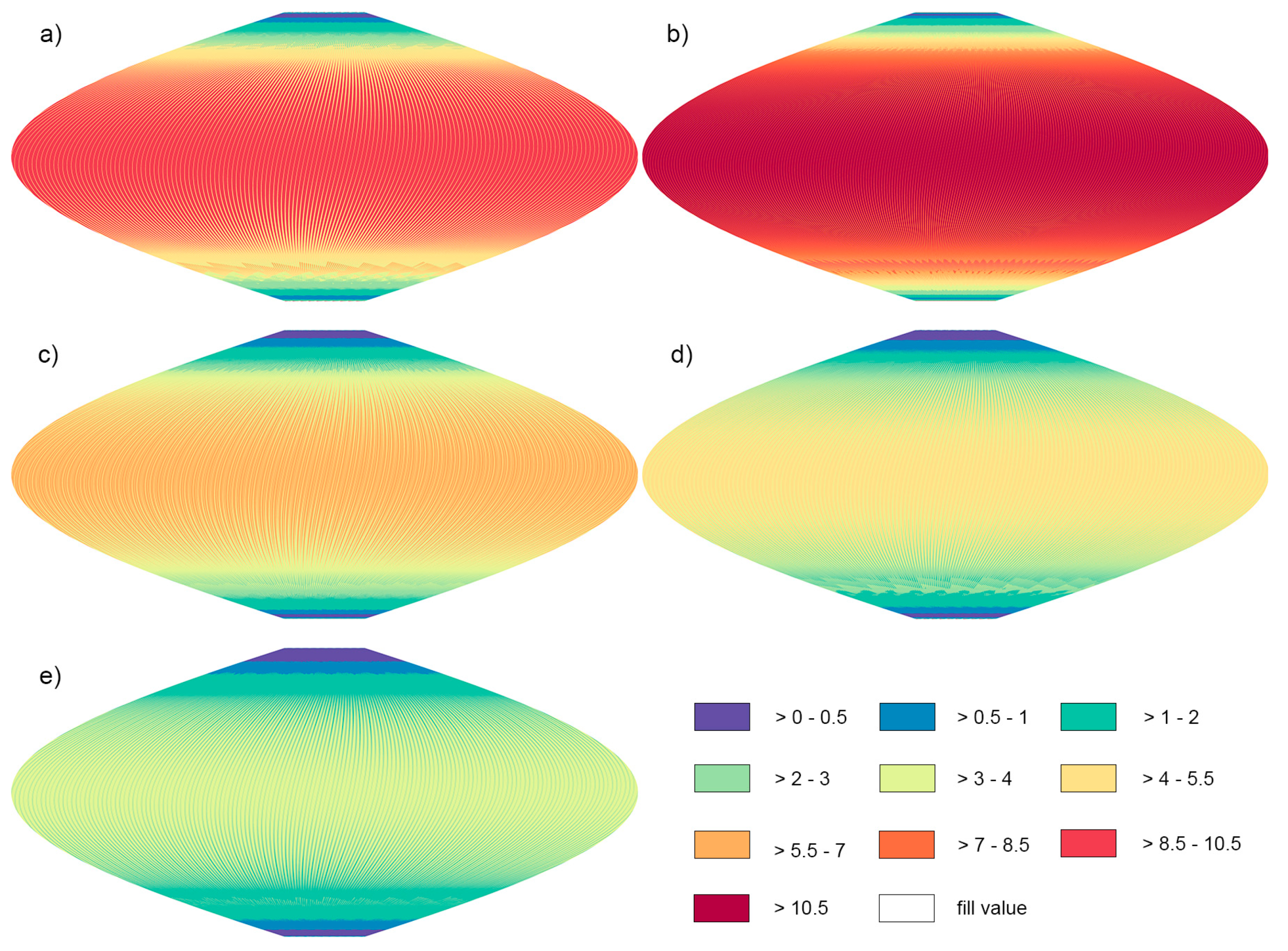
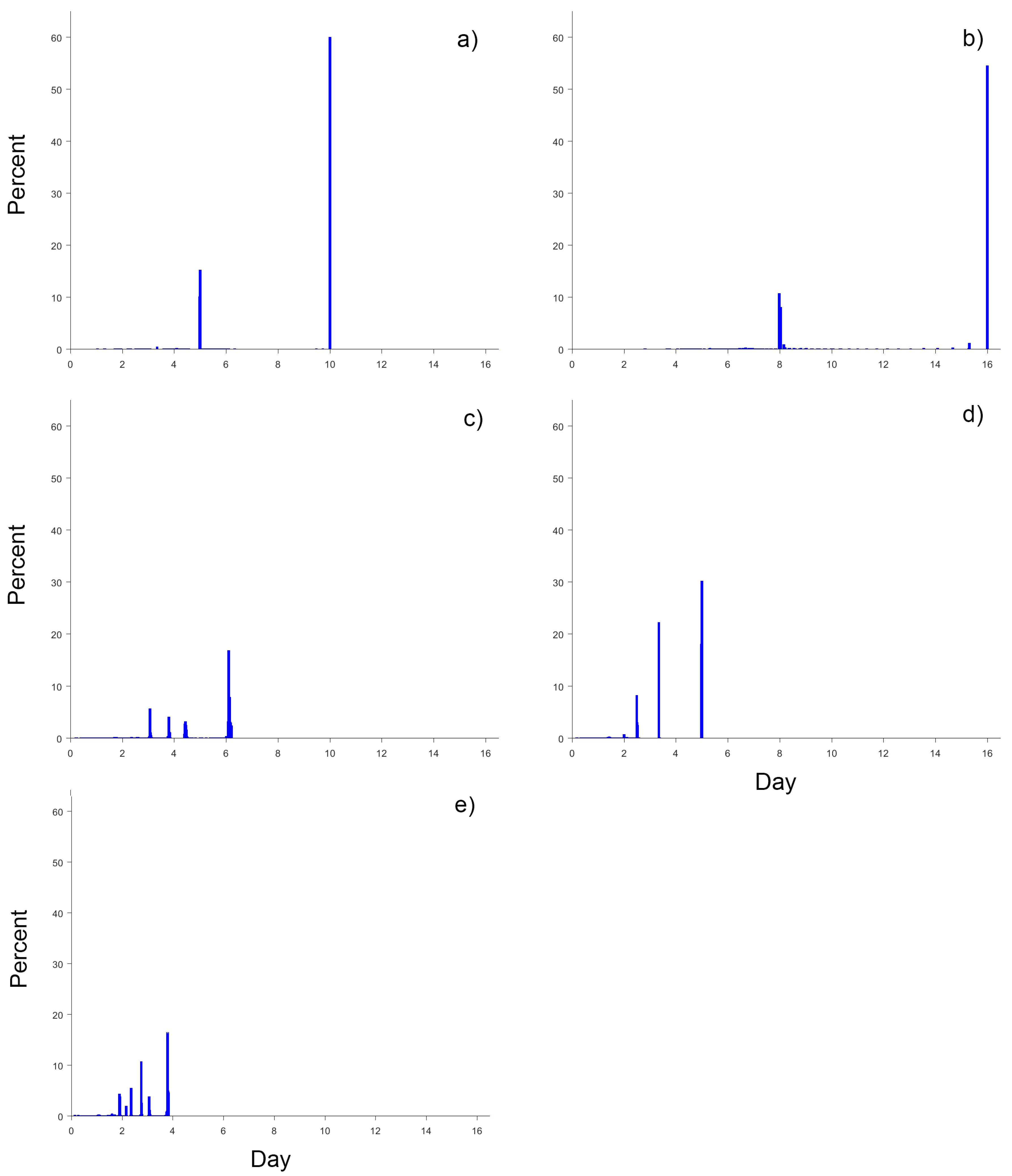
Figure 5 illustrates the average revisit interval calculated at each land grid point for 2016 considering the different sensor combinations. Shorter revisit intervals generally occur (Figure 5) where there are a greater number of annual observations (Figure 3). Figure 6 shows global histograms of the average revisit intervals; the histograms are negatively skewed with a greater frequency of large values.
Table 2 summarizes the global mean, median, and the first, second and third most frequent average revisit intervals for each of the different sensor combinations. When each sensor is considered alone, the globally most frequent average revisit intervals are the same as the median values and correspond to the sensor repeat cycles, i.e., 16 days (Landsat-8) and 10 days (Sentinel-2A or -2B), and occur for 54.6% (Landsat-8) and about 56% (either Sentinel-2) of the globe. The global mean average revisit intervals are smaller than the median values, due to the negatively skewed histograms, with values of about 12.1 and 7.8 days for Landsat-8 and either Sentinel-2 sensor, respectively.
When the sensors are combined the overlap of their different orbit swaths decreases the average revisit intervals. The globally most frequent average revisit intervals are 6.1 days (Landsat-8 and either Sentinel-2 sensor), 5.0 days (both Sentinel-2 sensors), and 3.8 days (all three sensors), and occur for about 14.8%, 29.0% and 11.8% of the globe, respectively. Landsat-8 and either Sentinel-2 sensor together have global mean and median average revisit intervals of about 4.6 and 4.5 days, respectively; the two Sentinel-2 sensors together have global mean and median average revisit intervals of 3.8 and 3.7 days, respectively; and, for all three sensors, the global mean and global median average revisit interval is about 2.9 days.
4.3. Minimum Revisit Intervals
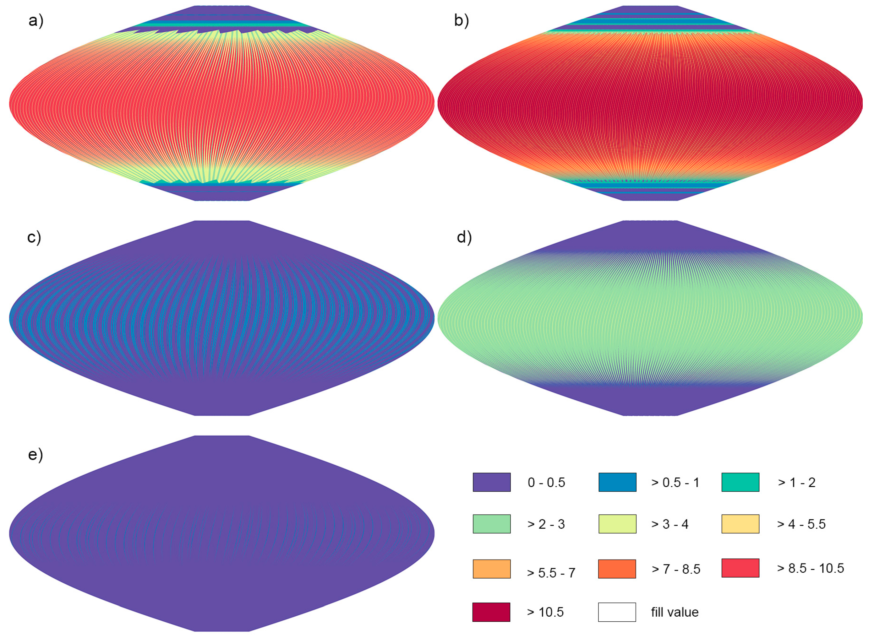
Figure 7 shows the minimum revisit interval calculated at each land grid point for 2016. The minimum revisit interval decreases further polewards and when more satellites are combined. Combination of the Landsat-8 and either Sentinel-2 sensor provides generally smaller minimum revisit intervals than when both Sentinel-2 sensors are considered due to the different phasing of the Landsat-8 and Sentinel-2 swaths. The global minimum revisit interval histograms (Figure 8) have 20 min bin widths and so only provide a broad depiction of the actual minimum revisit intervals and are more precisely summarized in Table 3.
For each sensor alone, the globally most frequent, as well as the median, minimum revisit intervals, are the sensor repeat cycles; these values occur for 48.7% (Landsat-8), 58.9% (Sentinel-2A) and about 61.6% (Sentinel-2B) of the globe (Table 3). As described in Section 3, each COVE KML granule corresponds to one minute in the track direction and so the revisit interval results have a reporting precision of ±1 min. The global minimum revisit histograms are negatively skewed (a greater frequency of large values) for each individual sensor and consequently the global mean minimum revisit intervals are smaller than the global median values and are about 11.1 days (Landsat-8) and 7.0 days (Sentinel-2).
When the different sensors are combined, the globally most frequent minimum revisit intervals are 16 min (Landsat-8 and either Sentinel-2), 3.0 days (both Sentinel-2 sensors), and 12 min (all three sensors), and occur for about 5.6%, 37.2% and 9.0% of the globe, respectively. Landsat-8 and either Sentinel-2 sensor data together provide global mean and median minimum revisit intervals of about 5 h 31 min and 17 min, respectively; the two Sentinel-2 sensors together provide global mean and median minimum revisit intervals of 2.2 and 3.0 days respectively; and for the three sensors the global mean and median minimum revisit intervals are 35 min and 14 min, respectively.
4.4. Maximum Revisit Intervals
Figure 9 shows the histogram of the maximum revisit intervals and Table 4 summarizes them. Global maps are not shown to save space but have similar spatial pattern as the minimum revisit interval global maps. The maximum revisit interval is constrained by the sensor repeat cycle, i.e., 16 days (Landsat-8) and 10 days (Sentinel-2), and so these values are common. When the two Sentinel-2 sensors are considered together, or when all three sensors are considered, the median and most frequent maximum revisit interval values are about 7.0 days. The most frequent maximum revisit intervals are about the same as the median values and occur for 56.8% (Landsat-8), 59.9% (Sentinel-2A), 61.7% (Sentinel-2B), 25.8% (Landsat-8 and Sentinel-2A), 28.7% (Landsat8 and Sentinel-2B), 28.6% (Sentinel-2A and Sentinel-2B), and 26.0% (all three sensors) of the globe.
5. Discussion
The analysis considered a global year of modeled sensor data and demonstrated that combination of Landsat-8 and Sentinel-2 generally increases the number of observations and reduces the revisit interval. In certain locations the number of useful surface observations will be smaller and the revisit interval greater than the reported results. This is because the analysis did not take into account cloud obscuration that precludes surface monitoring and is usually quite significant. For example, Kovalskyy and Roy [12] documented that 36% of a year of conterminous United States Landsat-8 observations were obscured by cloud and an additional 7% were obscured by cirrus. Globally, locations with very persistent cloud at the time of Landsat-5, Landsat-7, and MODIS overpass, have been observed to include Equatorial Africa, Amazonia, northern boreal regions, and Southeast Asia [1,4,10,11]. In addition, neither the Landsat-8 or Sentinel-2 sensors acquire data globally. For example, Landsat-8 does not acquire data over oceans and acquires 725 scenes per day out of a global average of 810 possible land scenes [27]. Similarly, the Sentinel-2 satellites will systematically acquire observations over land and coastal areas from −56° to 84° latitude including islands larger 100 km2, all the European Union islands, the Mediterranean Sea, and all inland water bodies and closed seas [28]. Future research to quantify the acquisition sensor frequencies considering the Landsat-8, Sentinel-2A and Sentinel-2B data archive and the degree of cloudiness when a global year of data are available is recommended.
The analysis was undertaken with respect to a global grid of 7201 × 3601 points spaced every 5.559752 km, equivalent to 0.05° at the Equator. This spacing is considerably smaller than the Landsat-8 185 km and Sentinel-2 290 km swath widths and was selected based on the analysis of Kovalskyy and Roy [4] who used it as it was sufficiently small to capture variable Landsat image locations imposed by Landsat-5 and Landsat-7 orbit drifts. As the Landsat-8 has improved geometry and more stable orbit compared to Landsat-5 and Landsat-7 [29,30], we do not anticipate orbit drift to have affected our results. We note however that Sentinel-2 and Landsat-8 data are currently misregistered relative to one another by 38 m (2σ) [31], although we do not anticipate this to be reflected in the COVE results and therefore can discount this issue for the purposes of this study.
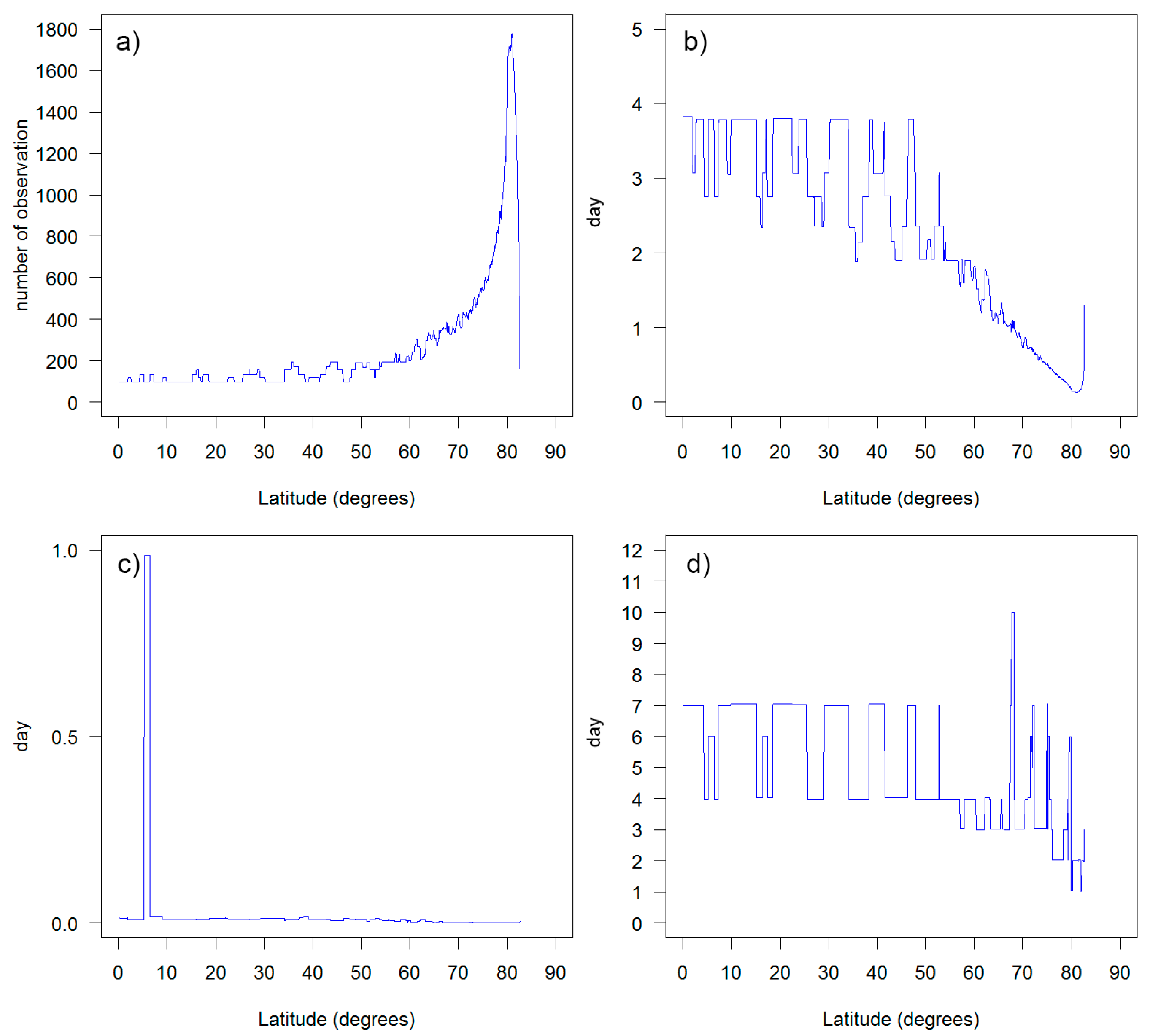
The global histograms of the annual number of observations and of the minimum, mean, and maximum revisit intervals were skewed (Figure 4, Figure 6, Figure 8 and Figure 9). Consequently, the summary global mean values are less representative than the summary global median values. Further, as each COVE KML granule corresponds to one minute in the track direction, the revisit interval results were rounded to the nearest minute. This resulted in an interval reporting precision of ±1 min. These issues are evident in Figure 10, which shows the annual number of observations, and the average, minimum and maximum revisit intervals calculated every 0.05° from the Equator to the North Pole along 0° longitude, considering all three sensors.
The different sensor orbits and swath widths mean that the annual number of observations and the average, minimum and maximum revisit intervals do not vary smoothly in space. This is evident in Figure 10. However, in general, up to latitude 80.9°N the number of observations increases and the average repeat interval decreases, especially above about 60°N where the different sensor swaths start to increasingly overlap laterally on the same day (Figure 1). The annual number of observations varies from 95 to 1779 and the average revisit varies from 183 min (3.05 h) to 5514 min (91.90 h, i.e., 3.83 days). Above 80.9°N, the sensors are close to their most poleward limit and fewer daytime observations occur.
The minimum and maximum revisit intervals illustrated in Figure 10, and in Section 4.3 and Section 4.4, are of interest because they define the degree that sensor observations may be near-coincident and their greatest temporal separation, respectively. The minimum revisit interval in Figure 10c varies from 1418 min (23.63 h) to zero minutes, with a reporting precision of ±1 min, and along the transect the median value is 14 min (the same as the global median 14 min minimum revisit interval reported in Table 3). Evidently, these results and the one illustrated in Figure 7e, illustrate that, at most latitudes, near-coincident Landsat-8, Sentinel-2A and Sentinel-2B observations will occur at some point in the year. For such small revisit internals the surface land cover and condition can be expected to be the same, although the surface may not be observed under constant atmospheric conditions at windy locations where atmospheric contamination is spatially heterogeneous. If the data are reliably atmospherically corrected and cloud-masked then the near coincident sensor observations will be useful for a number of applications. These include inter-sensor calibration [32,33], statistical examination of among-sensor spectral band-pass differences [19,34,35] and characterization of surface reflectance anisotropy [36,37]. Near coincident sensor data can be obtained opportunistically by searching the Sentinel-2 and Landsat-8 data archives or can be planned for using the COVE tool. The results also imply better than a 7 day revisit interval at most latitudes; the maximum revisit interval in Figure 10d varies from 1508 min (1.0 days) to 14,400 min (10.0 days), and along the transect the median value is 10,142 min (7.0 days).
The results of this study are encouraging for terrestrial monitoring applications that will utilize Landsat-8 and Sentinel-2 time series together. However, this study did not consider the different spatial and spectral resolutions of the Landsat-8 and Sentinel-2 sensors, which should also be considered when evaluating combined sensor data use.
6. Conclusions
This study demonstrated the utility of combining Sentinel-2 and Landsat-8 data to take advantage of the different sensor acquisition patterns to improve the observation temporal frequency. The main findings are that: (i) Landsat-8 and either Sentinel-2 sensor have a global median average revisit interval of 4.5 days and a global median minimum revisit interval of 17 min (±1 min); (ii) the two Sentinel-2 sensors together have a global median average revisit interval of 3.7 days and a global median minimum revisit interval of 3.0 days; (iii) Landsat-8, Sentinel-2A, and Sentinel-2B together have a global median average revisit interval of 2.9 days and a global median minimum revisit interval of 14 min (±1 min); and (iv) the maximum revisit interval is constrained by the sensor repeat cycle, the global median maximum revisit interval is 10.0 days for Landsat-8 and either Sentinel-2 sensor, and is 7.0 days when the two Sentinel-2 sensors or when all three sensors are considered together.
The temporal observation frequency improvements afforded by sensor combination quantified in this study are significant. For example, if we conservatively assume that 50% of observations are cloudy at the time of satellite overpass, then we can expect on average to have a global cloud-free observation better than every six days when Landsat-8, Sentinel-2A and Sentinel-2B are combined. This will benefit a large number of remote sensing applications, particularly land cover and change monitoring applications [5,6,18,38]. In addition, low temporal latency near-real time applications will become more feasible due to the greater certainty in obtaining cloud free imagery.
Acknowledgments
This research was funded by the NASA Land Cover/Land Use Change Multi-Source Land Imaging Science Program Grant NNX15AK94G, and by the U.S. Department of Interior, U.S. Geological Survey Grant G12PC00069. The NASA COVE team is thanked for the provision of the COVE Internet tool.
Author Contributions
J.L. and D.P.R. conceived the experiments; J.L. developed the code and processed the data and developed the graphics with assistance from D.P.R.; and D.P.R. structured and drafted the manuscript with assistance from J.L.
Conflicts of Interest
The authors declare no conflict of interest.
References
- Roy, D.P.; Lewis, P.; Schaaf, C.; Devadiga, S.; Boschetti, L. The global impact of cloud on the production of MODIS bi-directional reflectance model based composites for terrestrial monitoring. IEEE Geosci. Remote Sens. Lett. 2006, 3, 452–456. [Google Scholar] [CrossRef]
- Brown, M.E.; Pinzón, J.E.; Didan, K.; Morisette, J.T.; Tucker, C.J. Evaluation of the consistency of long-term NDVI time series derived from AVHRR, SPOT-vegetation, SeaWiFS, MODIS, and Landsat ETM+ sensors. IEEE Trans. Geosci. Remote Sens. 2006, 44, 1787–1793. [Google Scholar] [CrossRef]
- Fensholt, R.; Rasmussen, K.; Nielsen, T.T.; Mbow, C. Evaluation of earth observation based long term vegetation trends—Intercomparing NDVI time series trend analysis consistency of Sahel from AVHRR GIMMS, Terra MODIS and SPOT VGT data. Remote Sens. Environ. 2009, 113, 1886–1898. [Google Scholar] [CrossRef]
- Kovalskyy, V.; Roy, D.P. The global availability of Landsat 5 TM and Landsat 7 ETM+ land surface observations and implications for global 30 m Landsat data product generation. Remote Sens. Environ. 2013, 130, 280–293. [Google Scholar] [CrossRef]
- Drusch, M.; Del Bello, U.; Carlier, S.; Colin, O.; Fernandez, V.; Gascon, F.; Hoersch, B.; Isola, C.; Laberinti, P.; Martimort, P. Sentinel-2: ESA’s optical high-resolution mission for GMES operational services. Remote Sens. Environ. 2012, 120, 25–36. [Google Scholar] [CrossRef]
- Roy, D.P.; Wulder, M.; Loveland, T.; Woodcock, C.; Allen, R.; Anderson, M.; Helder, D.; Irons, J.; Johnson, D.; Kennedy, R.; et al. Landsat-8: Science and product vision for terrestrial global change research. Remote Sens. Environ. 2014, 145, 154–172. [Google Scholar] [CrossRef]
- Capderou, M. Satellites: Orbits and Missions; Springer: Paris, France, 2005. [Google Scholar]
- Wertz, J.R. Mission Geometry: Orbit and Constellation Design and Management: Spacecraft Orbit and Attitude Systems; Microcosm Press: El Segundo, CA, USA, 2009. [Google Scholar]
- Saboori, B.; Bidgoli, A.M.; Saboori, B. Multiobjective optimization in repeating sun-synchronous orbits design for remote-sensing satellites. J. Aerosp. Eng. 2013, 27, 04014027. [Google Scholar] [CrossRef]
- Sano, E.E.; Ferreira, L.G.; Asner, G.P.; Steinke, E.T. Spatial and temporal probabilities of obtaining cloud-free Landsat images over the Brazilian tropical savanna. Int. J. Remote Sens. 2007, 28, 2739–2752. [Google Scholar] [CrossRef]
- Ju, J.; Roy, D.P. The availability of cloud-free Landsat ETM+ data over the conterminous United States and globally. Remote Sens. Environ. 2008, 112, 1196–1211. [Google Scholar] [CrossRef]
- Kovalskyy, V.; Roy, D.P. A one year Landsat 8 conterminous United States study of cirrus and non-cirrus clouds. Remote Sens. 2015, 7, 564–578. [Google Scholar] [CrossRef]
- Wulder, M.A.; White, J.C.; Loveland, T.R.; Woodcock, C.E.; Belward, A.S.; Cohen, W.B.; Fosnight, G.; Shaw, J.; Masek, J.G.; Roy, D.P. The global Landsat archive: Status, consolidation, and direction. Remote Sens. Environ. 2016, 185, 271–283. [Google Scholar] [CrossRef]
- Whitcraft, A.K.; Becker-Reshef, I.; Killough, B.D.; Justice, C.O. Meeting earth observation requirements for global agricultural monitoring: An evaluation of the revisit capabilities of current and planned moderate resolution optical earth observing missions. Remote Sens. 2015, 7, 1482–1503. [Google Scholar] [CrossRef]
- Coppin, P.; Jonckheere, I.; Nackaerts, K.; Muys, B.; Lambin, E. Digital change detection methods in ecosystem monitoring: A review. Int. J. Remote Sens. 2004, 25, 1565–1596. [Google Scholar] [CrossRef]
- Roy, D.P.; Jin, Y.; Lewis, P.E.; Justice, C.O. Prototyping a global algorithm for systematic fire-affected area mapping using MODIS time series data. Remote Sens. Environ. 2005, 97, 137–162. [Google Scholar] [CrossRef]
- Verbesselt, J.; Hyndman, R.; Newnham, G.; Culvenor, D. Detecting trend and seasonal changes in satellite image time series. Remote Sens. Environ. 2010, 114, 106–115. [Google Scholar] [CrossRef]
- Zhu, Z. Change detection using landsat time series: A review of frequencies, preprocessing, algorithms, and applications. ISPRS J. Photogramm. Remote Sens. 2017, 130, 370–384. [Google Scholar] [CrossRef]
- Mandanici, E.; Bitelli, G. Preliminary Comparison of Sentinel-2 and Landsat 8 Imagery for a Combined Use. Remote Sens. 2016, 8, 1014. [Google Scholar] [CrossRef]
- Li, Z.; Zhang, H.K.; Roy, D.P.; Yan, L.; Huang, H.; Li, J. Landsat 15 m panchromatic assisted downscaling (LPAD) of 30 m reflective wavelength data to Sentinel-2 20 m resolution. Remote Sens. 2017, 9, 755. [Google Scholar]
- Kessler, P.D.; Killough, B.D.; Gowda, S.; Williams, B.R.; Chander, G.; Qu, M. CEOS Visualization Environment (COVE) Tool for Intercalibration of Satellite Instruments. IEEE Trans. Geosci. Remote Sens. 2013, 51, 1081–1087. [Google Scholar] [CrossRef]
- Irons, J.R.; Dwyer, J.L.; Barsi, J.A. The next Landsat satellite: The Landsat data continuity mission. Remote Sens. Environ. 2012, 122, 11–21. [Google Scholar] [CrossRef]
- European Space Agency (ESA). Sentinel-2 User Handbook; Revision 2; ESA Standard Document; ESA: Paris, France, 2015; 64p. [Google Scholar]
- Snyder, J.P. Flattening the Earth: Two Thousand Years of Map Projections; The University of Chicago Press: Chicago, IL, USA, 1993. [Google Scholar]
- O’Rourke, J. Computational Geometry in C, 2nd ed.; Cambridge University Press: Cambridge, UK, 1998. [Google Scholar]
- Knuth, D.E. The Art of Computer Programming: Sorting and Searching, 2nd ed.; Addison-Wesley: Reading, MA, USA, 1998; Volume 3. [Google Scholar]
- Loveland, T.R.; Irons, J.R. Landsat 8: The plans, the reality, and the legacy. Remote Sens. Environ. 2016, 185, 1–6. [Google Scholar] [CrossRef]
- Gascon, F.; Bouzinac, C.; Thépaut, O.; Jung, M.; Francesconi, B.; Louis, J.; Lonjou, V.; Lafrance, B.; Massera, S.; Gaudel-Vacaresse, A.; et al. Copernicus Sentinel-2A Calibration and Products Validation Status. Remote Sens. 2017, 9, 584. [Google Scholar] [CrossRef]
- Storey, J.; Choate, M.; Lee, K. Landsat 8 Operational Land Imager on-orbit geometric calibration and performance. Remote Sens. 2014, 6, 11127–11152. [Google Scholar] [CrossRef]
- Zhang, H.K.; Roy, D.P. Landsat 5 Thematic Mapper reflectance and NDVI 27-year time series inconsistencies due to satellite orbit change. Remote Sens. Environ. 2016, 186, 217–233. [Google Scholar] [CrossRef]
- Storey, J.; Roy, D.P.; Masek, J.; Gascon, F.; Dwyer, J.; Choate, M. A note on the temporary mis-registration of Landsat-8 Operational Land Imager (OLI) and Sentinel-2 Multi Spectral Instrument (MSI) imagery. Remote Sens. Environ. 2016, 186, 121–122. [Google Scholar]
- Teillet, P.M.; Barker, J.L.; Markham, B.L.; Irish, R.R.; Fedosejevs, G.; Storey, J.C. Radiometric cross-calibration of the Landsat-7 ETM+ and Landsat-5 TM sensors based on tandem data sets. Remote Sens. Environ. 2001, 78, 39–54. [Google Scholar] [CrossRef]
- Mishra, N.; Haque, M.O.; Leigh, L.; Aaron, D.; Helder, D.; Markham, B. Radiometric cross calibration of Landsat 8 operational land imager (OLI) and Landsat 7 enhanced thematic mapper plus (ETM+). Remote Sens. 2014, 6, 12619–12638. [Google Scholar] [CrossRef]
- Roy, D.P.; Kovalskyy, V.; Zhang, H.K.; Vermote, E.F.; Yan, L.; Kumar, S.S.; Egorov, A. Characterization of Landsat-7 to Landsat-8 reflective wavelength and normalized difference vegetation index continuity. Remote Sens. Environ. 2016, 185, 57–70. [Google Scholar] [CrossRef]
- Holden, C.E.; Woodcock, C.E. An analysis of Landsat 7 and Landsat 8 underflight data and the implications for time series investigations. Remote Sens. Environ. 2016, 185, 16–36. [Google Scholar] [CrossRef]
- Roy, D.P.; Zhang, H.K.; Ju, J.; Gomez-Dans, J.L.; Lewis, P.E.; Schaaf, C.B.; Sun, Q.; Li, J.; Huang, H.; Kovalskyy, V. A general method to normalize Landsat reflectance data to nadir BRDF adjusted reflectance. Remote Sens. Environ. 2016, 176, 255–271. [Google Scholar] [CrossRef]
- Roy, D.P.; Li, J.; Zhang, H.K.; Yan, L.; Huang, H.; Li, Z. Examination of Sentinel-2A multi-1 spectral instrument (MSI) reflectance anisotropy and the suitability of a general method to normalize MSI reflectance to nadir BRDF adjusted reflectance. Remote Sens. Environ. 2017, 199, 25–38. [Google Scholar] [CrossRef]
- Hansen, M.C.; Loveland, T.R. A review of large area monitoring of land cover change using Landsat data. Remote Sens. Environ. 2012, 122, 66–74. [Google Scholar] [CrossRef]
Figure 1.
Example committee on Earth Observation Satellite (CEOS) Visualization Environment (COVE) tool modeled orbit daytime swaths for 21 June 2016 (top) and 21 December 2016 (bottom) shown in the geographic (latitude/longitude) projection. The Landsat-8 swath is shown in Red, and the Sentinel-2A and Sentinel-2B swaths are shown in Green and Blue, respectively. The across-track lines show the COVE tool KML one-minute granule boundaries.

Figure 2.
Calculation of revisit intervals (t1, t2, t3, t4, t5, and t6) for example Sentinel-2A and Landsat-8 granules encompassing the same grid point location. In this example, the mean revisit interval is the average value of (t1, t2, t3, t4, t5, and t6) and the minimum and maximum revisit intervals are t4 and t5, respectively.

Figure 3.
The total annual number of satellite observations (1 January to 31 December 2016) for: (a) Sentinel-2A; (b) Landsat-8; (c) Landsat-8 and Sentinel-2A; (d) Sentinel-2A and Sentinel-2B; and (e) Landsat-8, Sentinel-2A and Sentinel-2B. Global results derived at 7201 × 3601 points spaced every 5.559752 km, equivalent to 0.05° at the Equator, in the equal area sinusoidal projection.

Figure 4.
Histograms of the total number of observations globally for: (a) Sentinel-2A; (b) Landsat-8; (c) Landsat-8 and Sentinel-2A; (d) Sentinel-2A and Sentinel-2B; and (e) Landsat-8, Sentinel-2A and Sentinel-2B. The histogram bin widths are set as 0–1, 2–3, 4–5, …, 448–449, and the percentages denote the percentage in each bin. Results derived from the global 0.05° data (Figure 3).
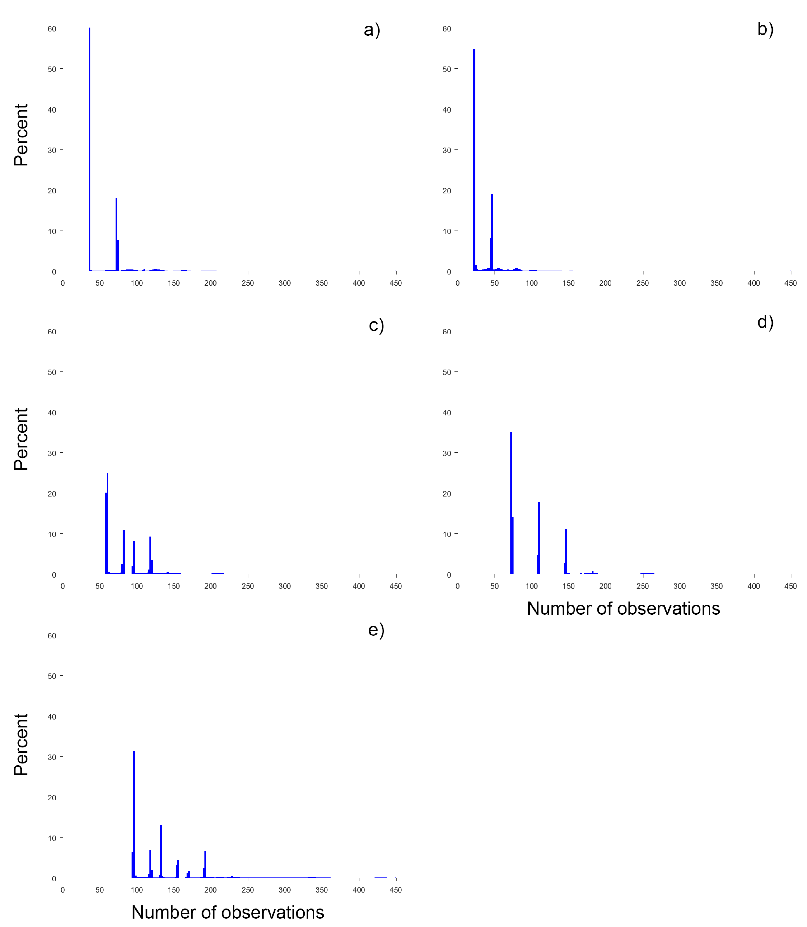
Figure 5.
The average satellite revisit interval (days) from 1 January to 31 December 2016 for: (a) Sentinel-2A; (b) Landsat-8; (c) Landsat-8 and Sentinel-2A; (d) Sentinel-2A and Sentinel-2B; and (e) Landsat-8, Sentinel-2A and Sentinel-2B. Global results derived at 7201 × 3601 points spaced every 5.559752 km, equivalent to 0.05° at the Equator, in the equal area sinusoidal projection.

Figure 6.
Histograms of the average revisit interval globally for: (a) Sentinel-2A; (b) Landsat-8; (c) Landsat-8 and Sentinel-2A; (d) Sentinel-2A and Sentinel-2B; and (e) Landsat-8, Sentinel-2A and Sentinel-2B. The histogram bin widths correspond to 20 min, and the percentages denote the percentage in each bin. Results derived from the global 0.05° data (Figure 5).

Figure 7.
The minimum satellite revisit interval (days) from 1 January to 31 December 2016 for: (a) Sentinel-2A; (b) Landsat-8; (c) Landsat-8 and Sentinel-2A; (d) Sentinel-2A and Sentinel-2B; and (e) Landsat-8, Sentinel-2A and Sentinel-2B. Global results derived at 7201 × 3601 points spaced every 5.559752 km, equivalent to 0.05° at the Equator, in the equal area sinusoidal projection.

Figure 8.
Histograms of the minimum revisit interval globally for: (a) Sentinel-2A; (b) Landsat-8; (c) Landsat-8 and Sentinel-2A; (d) Sentinel-2A and Sentinel-2B; and (e) Landsat-8, Sentinel-2A and Sentinel-2B. The histogram bin widths correspond to 20 min, and the percentages denote the percentage in each bin. Results derived from the global 0.05° data (Figure 7).
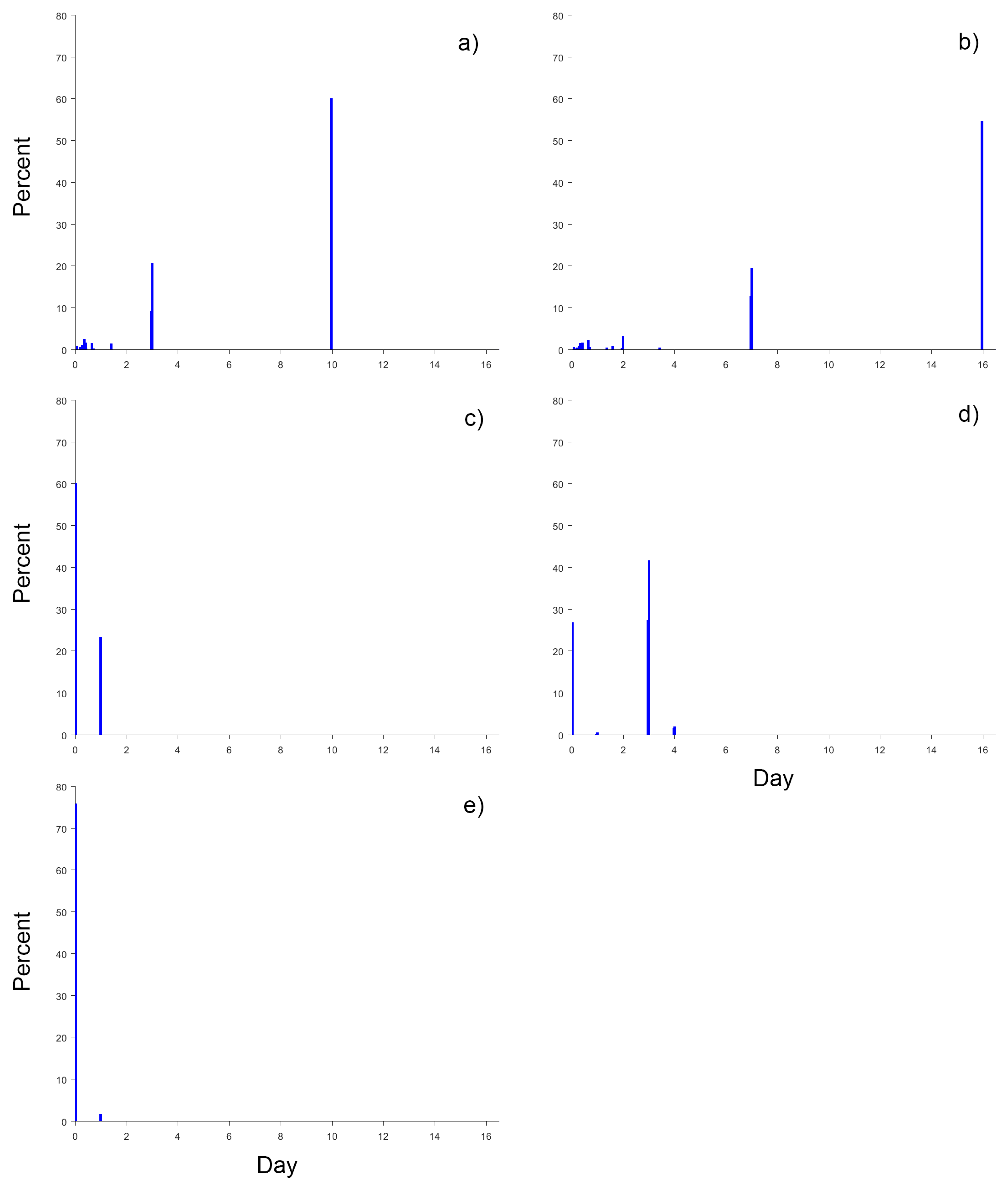
Figure 9.
Histograms of the maximum revisit interval globally for: (a) Sentinel-2A; (b) Landsat-8; (c) Landsat-8 and Sentinel-2A; (d) Sentinel-2A and Sentinel-2B; and (e) Landsat-8, Sentinel-2A and Sentinel-2B. The histogram bin widths correspond to 20 min, and the percentages denote the percentage in each bin.
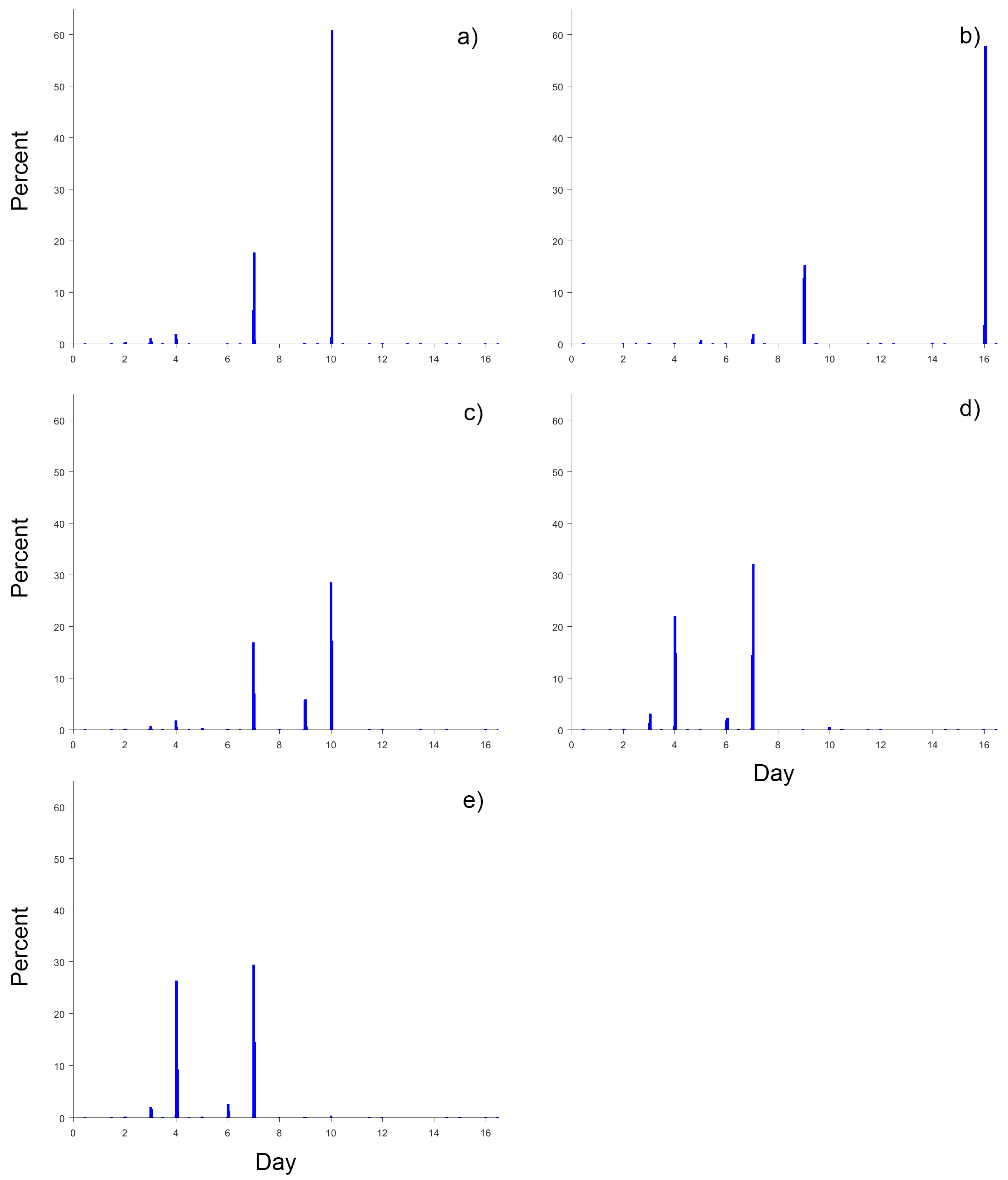
Figure 10.
Latitudinal transects, defined every 0.05° from 0° to 90° N along the prime meridian (0° longitude), of the global annual results considering Landsat-8, Sentinel-2A and Sentinel-2B: (a) total number of observations (from Figure 3e); (b) average revisit interval (from Figure 5e); (c) minimum revisit interval (Figure 7e); and (d) maximum revisit interval.

Table 1.
Global summary statistics (mean and median) of the total number of observations from 1 January to 31 December 2016 for different satellite combinations. In addition, the first, second and third most frequent number of observations are shown with the percentage of global grid points with that number of observations in parenthesis. Results derived from the global 0.05° data (Figure 3).
| Landsat-8 | Sentinel-2A | Sentinel-2B | Landsat-8 Sentinel-2A | Landsat-8 Sentinel-2B | Sentinel-2A Sentinel-2B | Landsat-8 Sentinel-2A Sentinel-2B | |
|---|---|---|---|---|---|---|---|
| Mean | 39.8 | 61.6 | 61.3 | 101.4 | 101.0 | 122.9 | 162.6 |
| Median | 23 | 37 | 37 | 81 | 81 | 100 | 127 |
| most frequent total value | 23 (47.9%) | 37 (35.9%) | 37 (36.3%) | 60 (24.2%) | 60 (23.6%) | 73 (30.2%) | 96 (21.1%) |
| 2nd most frequent total value | 46 (18.8%) | 73 (15.3%) | 73 (15.1%) | 119 (6.4%) | 119 (6.8%) | 110 (17.7%) | 133 (9.6%) |
| 3rd most frequent total value | 54 (0.8%) | 110 (0.4%) | 110 (0.4%) | 82 (0.2%) | 82 (0.2%) | 146 (0.3%) | 118 (0.1%) |
Table 2.
Global summary statistics (mean and median) of the average satellite revisit interval from 1 January to 31 December 2016 for different satellite combinations reported in decimal days (to 3 d.p.). In addition, the first, second and third most frequent average satellite revisit interval values are tabulated with the percentage of global grid points with that value in parenthesis. Results derived from the global 0.05° data (Figure 5).
| Landsat-8 | Sentinel-2A | Sentinel-2B | Landsat-8 Sentinel-2A | Landsat-8 Sentinel-2B | Sentinel-2A Sentinel-2B | Landsat-8 Sentinel-2A Sentinel-2B | |
|---|---|---|---|---|---|---|---|
| Mean | 12.130 | 7.771 | 7.820 | 4.593 | 4.611 | 3.795 | 2.835 |
| Median | 16.000 | 10.000 | 10.000 | 4.456 | 4.456 | 3.667 | 2.858 |
| most frequent total value | 16.000 (54.6%) | 10.000 (55.5%) | 10.000 (56.6%) | 6.097 (14.8%) | 6.097 (14.9%) | 5.000 (29.0%) | 3.792 (11.8%) |
| 2nd most frequent total value | 7.972 (10.7%) | 5.000 (14.0%) | 5.000 (15.1%) | 3.055 (1.8%) | 3.055 (2.1%) | 3.333 (13.6%) | 2.750 (3.1%) |
| 3rd most frequent total value | 15.306 (1.1%) | 3.333 (0.5%) | 3.333 (0.5%) | 3.800 (0.1%) | 3.800 (0.1%) | 2.486 (0.2%) | 2.347 (0.2%) |
Table 3.
Global summary statistics (mean and median) of the minimum satellite revisit interval from 1 January to 31 December 2016 for different satellite combinations reported in decimal days (to 3 d.p.) or hours and minutes (to the closest minute). In addition, the first, second and third most frequent minimum satellite revisit interval values are tabulated with the percentage of global grid points with that value in parenthesis. Results derived from the global 0.05° data (Figure 7).
| Landsat-8 | Sentinel-2A | Sentinel-2B | Landsat-8 Sentinel-2A | Landsat-8 Sentinel-2B | Sentinel-2A Sentinel-2B | Landsat-8 Sentinel-2A Sentinel-2B | |
|---|---|---|---|---|---|---|---|
| Mean | 11.101 | 6.931 | 7.038 | 5 h, 31 min | 5 h, 48 min | 2.209 | 35 min |
| Median | 15.958 | 9.958 | 9.958 | 17 min | 17 min | 2.965 | 14 min |
| most frequent total value | 15.958 (48.7%) | 9.958 (58.9%) | 9.958 (61.6%) | 16 min (5.6%) | 16 min (5.7%) | 3.000 (37.2%) | 12 min (9.0%) |
| 2nd most frequent total value | 7.000 (19.2%) | 3.000 (15.9%) | 3.000 (15.7%) | 1.000 (2.8%) | 1.000 (2.9%) | 12 min (16.5%) | 0.986 (0.31%) |
| 3rd most frequent total value | 1.986 (3.1%) | 0.347 (2.5%) | 0.347 (2.5%) | 3.000 (0.0%) | 3.000 (0.0%) | 4.000 (1.9%) | 2.931 (0.0%) |
Table 4.
Global summary statistics (mean and median) of the maximum satellite revisit interval from 1 January to 31 December 2016 for different satellite combinations reported in decimal days (to 3 d.p.). In addition, the first, second and third most frequent maximum satellite revisit interval values are tabulated with the percentage of global grid points with that value in parenthesis.
| Landsat-8 | Sentinel-2A | Sentinel-2B | Landsat-8 Sentinel-2A | Landsat-8 Sentinel-2B | Sentinel-2A Sentinel-2B | Landsat-8 Sentinel-2A Sentinel-2B | |
|---|---|---|---|---|---|---|---|
| Mean | 14.092 | 9.680 | 9.680 | 9.545 | 9.531 | 6.570 | 6.560 |
| Median | 16.042 | 10.042 | 10.042 | 10.000 | 10.000 | 7.001 | 7.001 |
| most frequent total value | 16.042 (56.8%) | 10.042 (59.9%) | 10.042 (61.7%) | 10.000 (25.8%) | 10.000 (28.7%) | 7.042 (28.6%) | 7.000 (26.0%) |
| 2nd most frequent total value | 9.042 (13.2%) | 7.028 (17.7%) | 7.028 (16.4%) | 6.986 (16.0%) | 6.986 (15.4%) | 4.000 (20.6%) | 4.000 (24.4%) |
| 3rd most frequent total value | 7.042 (1.9%) | 3.986 (1.8%) | 3.986 (1.8%) | 9.000 (5.9%) | 9.000 (5.9%) | 3.042 (3.1%) | 6.0 (2.6%) |
© 2017 by the authors. Licensee MDPI, Basel, Switzerland. This article is an open access article distributed under the terms and conditions of the Creative Commons Attribution (CC BY) license (http://creativecommons.org/licenses/by/4.0/).
Share and Cite
MDPI and ACS Style
Li, J.; Roy, D.P. A Global Analysis of Sentinel-2A, Sentinel-2B and Landsat-8 Data Revisit Intervals and Implications for Terrestrial Monitoring. Remote Sens. 2017, 9, 902. https://doi.org/10.3390/rs9090902
AMA Style
Li J, Roy DP. A Global Analysis of Sentinel-2A, Sentinel-2B and Landsat-8 Data Revisit Intervals and Implications for Terrestrial Monitoring. Remote Sensing. 2017; 9(9):902. https://doi.org/10.3390/rs9090902
Chicago/Turabian StyleLi, Jian, and David P. Roy. 2017. "A Global Analysis of Sentinel-2A, Sentinel-2B and Landsat-8 Data Revisit Intervals and Implications for Terrestrial Monitoring" Remote Sensing 9, no. 9: 902. https://doi.org/10.3390/rs9090902
Note that from the first issue of 2016, this journal uses article numbers instead of page numbers. See further details here.