A Multiscale Deeply Described Correlatons-Based Model for Land-Use Scene Classification

Abstract

Research efforts in land-use scene classification is growing alongside the popular use of High-Resolution Satellite (HRS) images. The complex background and multiple land-cover classes or objects, however, make the classification tasks difficult and challenging. This article presents a Multiscale Deeply Described Correlatons (MDDC)-based algorithm which incorporates appearance and spatial information jointly at multiple scales for land-use scene classification to tackle these problems. Specifically, we introduce a convolutional neural network to learn and characterize the dense convolutional descriptors at different scales. The resulting multiscale descriptors are used to generate visual words by a general mapping strategy and produce multiscale correlograms of visual words. Then, an adaptive vector quantization of multiscale correlograms, termed multiscale correlatons, are applied to encode the spatial arrangement of visual words at different scales. Experiments with two publicly available land-use scene datasets demonstrate that our MDDC model is discriminative for efficient representation of land-use scene images, and achieves competitive classification results with state-of-the-art methods.

1. Introduction

High-Resolution Satellite (HRS) images are increasingly available and therefore are playing an ever-more important role in land-use classification [1]. HRS images provide more of the appearance and spatial arrangement information needed in land-use scene category recognition [2]. It is usually difficult, however, to recognize land-use scene categories because they often comprise of multiple land covers or ground objects [3,4,5,6,7,8,9,10,11], such as airports with airplanes, runways and grass. Land-use scene categories are largely affected and determined by human social activities. Thus, the land-use scene recognition and classification in HRS images are based on a priori knowledge. Subsequently, the traditional pixel-based [12] and low-level feature-based image classification techniques [13,14] are inadequate for land-use scene classification.

The Bag-of-Visual-Words (BoVW) model, extremely popular in image analysis and classification [15,16,17,18], provides an efficient solution for land-use scene classification. The BoVW model, initially proposed for text categorization, treats an image as a collection of unordered appearance descriptors, and represents images with the frequency of “visual words” that are constructed by quantizing local features with a clustering method (e.g., k-means) [15]. The original BoVW method discards the spatial order of the local features and severely limits the descriptive capability of image representation. Therefore, many variant methods [4,19,20,21,22] based on the BoVW model have been developed for improving the ability to depict the spatial relationships of local features. These methods rely heavily on low-level feature descriptors for generating visual words. However, these low-level features, such as Scale-Invariant Feature Transform (SIFT) [23] or Histograms of Oriented Gradients (HOGs) [24], are unreliable and often fail to accurately characterize the complex land-use scenes found in HRS images [25].

Convolutional Neural Networks (CNNs), a hierarchical network invariant to image translations, have achieved great success in image classification [26], detection [27] and segmentation [28] on several benchmarks [29]. CNN is a biologically inspired multi-stage architecture composed of convolutional layers, pooling layers, and fully-connected layers. The key to success is the ability to learn increasingly complex transformations of the input and capture invariances from large labelled datasets [30]. Importantly, much of the recent work [31,32,33,34,35,36] has demonstrated that CNNs pre-trained on large datasets such as ImageNet [37] contain general-purposed feature extractors and can be transferable to many other domains. This is very helpful in the land-use scene classification because of the difficulty of training a deep CNN with a small number of training samples. Many approaches utilize the outputs of a deep and fully-connected layer as features to achieve transfer in CNNs. These methods, however, must fit the input image to a fixed size rendering it compatible with fully connected layers, either via cropping [26] or via warping [33]. The deeper layers may be more domain-specific, and therefore potentially less transferrable than shallower layers. Cimpoi et al. [30] proposed a representation method using the convolutional layer of a CNN as filter bank and Fisher Vector (FV) as a pooling mechanism. This method can process any image size by convolutional layers and avoid costly resizing operations. However, the pooling mechanism is orderless, and thus does not capture information concerning spatial layout, which has limited descriptive ability in land-use scene classification. Spatial pyramid pooling [19,38,39,40,41,42] (popularly known as spatial pyramid matching or SPM [19]) can incorporate spatial information and accept any size of input images by partitioning the image into increasingly fine subregions and computing the histograms of local features found inside each subregion. This pooling method was designed for natural image scene classification using ordered regular grids that incorporate spatial information into the representation, and therefore are sensitive to the rotation of image scenes. This sensitivity problem inevitably causes misclassification of scene images, especially for land-use scene images, and influences classification performance.

Motivated by the concept of color correlograms [43], Savarese et al. proposed a correlaton model to capture spatial co-occurrence information by correlograms of features. Correlograms are easy to compute and robust to occlusions, and can encode both local and global spatial arrangement information [44]. The correlaton method uses correlograms of local features to model the typical spatial correlation of visual words and applies adaptive vector quantization to compact correlograms without loss of discrimination [20,44]. However, the correlograms used in these methods are sensitive with respect to scale. Therefore, we proposed a Multiscale Deeply Described Correlatons (MDDC)-based model to incorporate appearance and spatial information at multiple scales for land-use scene classification. In the MDDC, we learn deeply described visual words through CNNs at different scales, so that complex land-use scenes can be described more robustly using these multiscale deep features. A mapping strategy is applied to label each multiscale local feature and compute the corresponding multiscale correlogram of the visual words for encoding both local and global spatial information at different scales. We apply adaptive vector quantization of multiscale correlograms to achieve a compact spatial representation without loss of discrimination. Experiments were conducted based on two public ground truth image datasets, manually extracted from publicly available high-resolution overhead imagery. Experimental results show that the MDDC-based model using CNN and multiscale correlograms is a simple yet effective way to represent the land-use scene images and achieves high classification accuracies.

The remainder of this paper is organized as follows: Section 2 introduces the proposed MDDC-based model for land-use scene classification. The experimental results and analysis are presented in Section 3, followed by an analysis and discussion in Section 4. In Section 5, some concluding remarks are presented and perspectives on future work close the paper.

2. The Proposed Method

In this section, we give a detailed description of land-use scene representation and classification in the MDDC framework. The proposed approach includes four main components: visual words encoding, correlogram extraction, correlaton encoding, and classification. In the visual words encoding step, dense convolutional features are extracted at multiple scales using pre-trained CNNs such as VGG (Visual Geometry Group Net) neural network, and features are flattened into vectors for deeply described visual word generation. In the correlogram extraction step, a general mapping strategy is applied to label each feature and compute the correlograms of visual words at different scales. In the correlaton encoding step, an adaptive vector quantization of multiscale correlograms, called a multiscale correlaton, was applied to achieve a compact spatial representation without loss of discrimination. In the classification step, with a concatenated histogram of visual words and multiscale correlatons, linear Support Vector Machine (SVM) classifiers are trained for land-use scene classification. Figure 1 illustrates the flowchart of this framework.

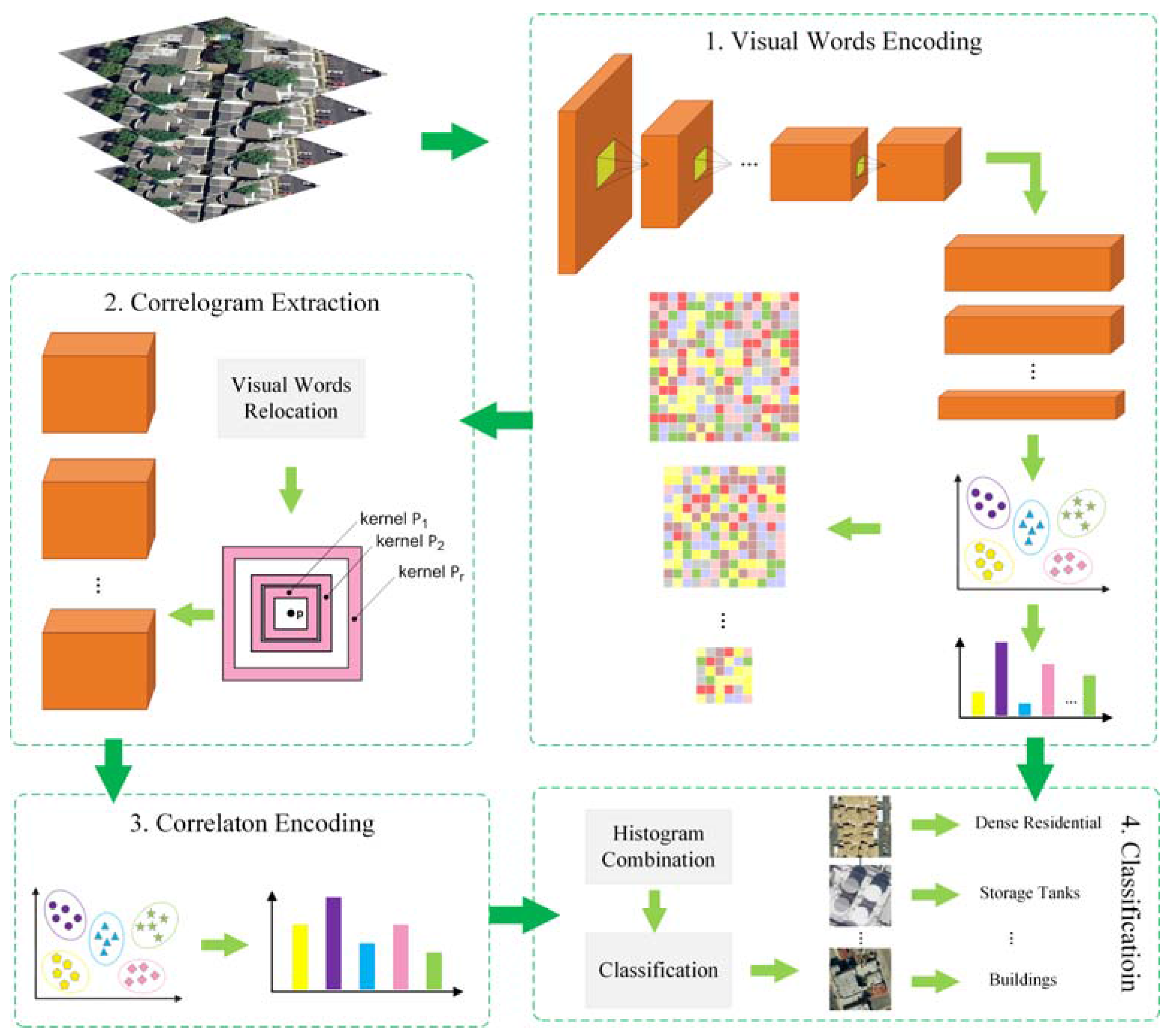
2.1. Multiscale Deeply Described Visual Words Encoding

The original concept of CNN was biologically inspired by “neocognitron” [45], a hierarchical network with invariance to image translations. LeCun et al. [46] refined the CNN architecture and successfully applied in character recognition. The CNN framework is organized in layers, and the first few stages are composed of convolutional layers and pooling layers. The convolutional layers learn the weights of filters to produce convolutional information of the input image. The first convolutional layer only learns locally low-level features for working on a small image window. The deeper convolutional layer learns more robust and complex features from low-level features for a broader view. Pooling layers perform a down-sampling operation to reduce the size of image by computing the maximum on a local region. Fully connected layers connect all neurons in the previous pooling layers and convolutional layers to every single neuron of itself for better summarized results and accurate classification.

In this paper, the deeply described visual words are computed on the output of a single convolutional layer of the CNN, such as the last convolutional layer. The input images need not be rescaled to a specific size for the non-required computation of fully connected layers. Thus, we can extract the dense convolutional features at different scales and pooled them as in SIFT. Specifically, we construct multiscale dense convolutional features with $S$ scales by subsampling/supersampling original HRS images and extracting single-scale convolutional features. Then, a visual vocabulary containing K entries was formed by a pooling method such as k-means [15] using a random subset of features at all scales from the training set.

Let $X={[X^1,X^2,\dots ,X^S]}^T$ be a set of descriptors obtained through dense convolutional feature representation in an N-dimensional feature space at $S$ different scales. The single-scale dense convolutional descriptors $X^s$ is defined as follows:

$$X^s={[x_1^s,x_2^s,\dots ,x_{M_s}^s]}^T\in {ℝ}^{M_s\times N}, s=1,\dots ,S$$

(1)

where $x_m^s$ is the $m^{th}$ descriptor and $M_s$ is the number of descriptors at scale $s$. A dictionary $D$ has $K$ training atoms ${\{d_k\}}_{k=1, 2,\dots K}$, each of which is an N-dimensional vector. The dictionary is formed by collecting all the multiscale descriptors $X$ from the training set, selecting a random subset of features, and applying a pooling method to encode these local descriptors. In different pooling methods, the deeply described visual word encoding is transformed into dictionary generation problem that is solved as different optimization problems. Let $V={[V^1,V^2,\dots ,V^S]}^T$ be the multiscale coefficient matrix and a single-scale coefficient matrix $V^s$ is represented as follows:

$$V^s={[v_1^s,v_2^s,\dots ,v_{M_s}^s]}^T\in {ℝ}^{M_s\times K}, s=1,\dots ,S$$

(2)

where $v_m^s$ is the cluster membership indicator for the descriptor $x_m^s$. Once the dictionary $D$ is pre-trained and fixed, $V^s$ can be computed by applying the corresponding encoding of $X^s$. Let $|v_m^s|$ be the $l_1$-norm of $v_m^s$, or the summation of the absolute value of each element in $v_m^s$; the k-means adopted in this paper constrains $|v_m^s|=1$, and restricts only non-zero entry in $v_m^s$. Finally, an image feature vector $u$ is computed by using a corresponding pooling function and adding up all the elements $v_m^s$ as follows:

$$u={\displaystyle \sum }_{s=1}^S{\displaystyle \sum }_{m=1}^M{v}_m^s\in {ℝ}^{1\times K}$$

(3)

Thus, we obtained multiscale bag-of-visual words representation for each image, which is an appearance-based representation. Mathematically, this representation of an image is the frequency or histogram of multiscale visual words in the vocabulary.

2.2. Multiscale Correlograms

A traditional correlogram is a matrix expressing spatial co-occurrences of features, encoding both the local and global spatial relationship of visual words, and is robust with respect to basic geometric transformations and occlusions [43]. For a multiscale deeply described visual word, a label will be assigned as a visual word index for each descriptor at different scales. The number of such labels is $K$, which equals to the size of visual vocabulary. Let $\Pi$ be a kernel (or image mask), and ${\Pi }_r$ be the $r^{th}$ kernel. The number of occurrences of visual words labeled as $l_p$ and $l_q$ at scale $s$ within the kernel ${\Pi }_r$ defined as $h^s({\Pi }_r,l_p,l_q)$, for $l_p=1\dots K,l_q=1\dots K,r=1\dots T,s=1\dots S$, where T is the number of kernels. Then, a correlogram at scale $s$ that is a $K\times K\times T$ matrix $C(I)$ is extracted from the value of $h^s({\Pi }_r,l_p,l_q)$.

In this paper, deeply described visual words are learned by k-means, while each descriptor is given a label with a corresponding entry index in the dictionary. We used a maximum map strategy [47], which assigns the index of maximum non-zero entry in the coefficient matrix to the label, for the visual words pooling method. Thus, the single-scale coefficient matrix $V^s\in {ℝ}^{M_s\times K}$ using k-means is represented as follows.

$$V^s={[v_1^s,v_2^s,\dots ,v_{M_s}^s]}^T\in {ℝ}^{M_s\times K},subject to: |v_m^s|=1,and{v}_{mi}^s\in \{0, 1\}$$

(4)

where $v_{mi}^s$ is the matrix element of $m^{th}$ row and $i^{th}$ column of $V^s$, and there is only one entry that is 1 and others are 0 in $v_m^s$. The label of a descriptor is represented by the index of non-zero. For example, if the non-zero entry in $v_m^s$ is $v_{mi}^s$, the label will be $i$. The spatial co-occurrences of a pair of deeply described visual words are easily exploited using the labels of descriptors.

Since multiscale deeply described visual words are constructed, we should consider the spatial correlation of visual words at different scales. We can calculate the correlograms at each scale separately and integrate them into a larger set. However, if we directly extract correlograms from descriptors explored in the subsampling/supersampling images, we must select parameters for correlograms at each scale. Therefore, we relocate the descriptors by rescaling the images of each scale to the size of original images. In this way, we can apply same parameters of correlograms for different scales.

Specifically, for each kernel ${\Pi }_r$, we define $W^s({\Pi }_r,p,q,i,j)$ to indicate the co-occurrence of visual word $p$ and $q$ in descriptors $i$ and $j$ at scale $s$ as follows:

$$W^s({\Pi }_r,p,q,i,j)= v_{ip}^s{v}_{jq}^s$$

(5)

We define $H^s({\Pi }_r,p)$ as a corresponding local histogram for each kernel at scale $s$, and $q^{th}$ element $H^s({\Pi }_r,p,q)$ are defined as follows:

$$H^s({\Pi }_r,p,q)={\displaystyle \sum }_{i=1}^M{\displaystyle \sum }_{j=1}^M{W}^s({\Pi }_r,p,q,i,j)$$

(6)

We compute the average local histogram ${\widehat{H}}^s({\Pi }_r,p)$, which describes the average distribution of visual words with respect to visual word $p$ within the region ${\Pi }_r$ at scale $s$ as follows:

$${\widehat{H}}^s({\Pi }_r,p)=\frac{H^s({\Pi }_r,p)}{{\sum }_{q=1}^K{H}^s({\Pi }_r,p,q)}$$

(7)

We denote $j^{th}$ elements of ${\widehat{H}}^s({\Gamma }_r, i)$ as $\widehat{h}({\Gamma }_r, i, j)$ for $i=1\dots K,j=1\dots K,r=1\dots T$. As a result, a correlogram at scale $s$, which is a $K\times K\times T$ matrix $C^s$, can be obtained by collecting the values ${\widehat{h}}^s({\Gamma }_r, i, j)$. We define the single-scale correlogram element $E^s(i,j)$, which is obtained from the $i^{th}$ row and $j^{th}$ column of $C^s$, as a $1\times T$ vector. Each single-scale correlogram can be regarded as a set of $K\times K$ correlogram elements. A multiscale correlogram is expressed as:

$$C=[C^s,C^s, \dots ,C^s]\in {ℝ}^{(K\times K\times S)\times T}, s=1,\dots ,S$$

(8)

and a single correlogram $C^s$ is represented as:

$$C^s=[E^s(1,1),\dots ,E^s(1,K),\dots ,E^s(K,1),\dots ,E^s(K,K)]\in {ℝ}^{(K\times K)\times T}$$

(9)

The correlogram element $E^s(i,j)$ can expresses how the co-occurrence of a pair of visual words $i$ and $j$ changes with different kernel radii. Thus, correlograms can encode both local and global spatial information at multiple scales.

2.3. Modeling Land-Use Scene by Multiscale Correlotons

The appearance-based representation of a land-use scene image is generated using multiscale dense convolutional features and corresponding pooling function. We extract corresponding $1\times K$ single-scale correlogram elements for each pair of visual words at the same scale. Then, all the single-scale correlogram elements at different scales are collected and clustered with k-means. The cluster centers, termed multiscale correlatons, are quantization of these multiscale correlogram elements, and the set of these cluster centers are correlaton vocabulary. The spatial information in a land-use scene image is represented as a histogram of multiscale correlaton occurrences by mapping the multiscale correlogram elements from each image to the corresponding correlaton vocabulary. Therefore, multiscale correlatons compress spatial co-occurrences of visual words at multiple scales without loss of discrimination accuracy. Due to the compactness, multiscale correlatons can improve efficiency and alleviate over fitting problems. Finally, a concatenated histogram of visual words and multiscale correlatons is classified using linear SVM classifiers.

3. Experiments and Analysis

In this section, we provide the experimental setups, and discuss the results on two public datasets. We conducted several groups of experiments to investigate the effectiveness of the MDDC-based representation for land-use scene classification.

3.1. Experimental Setup

We evaluated our proposed model on two public land-use scene datasets, which were:

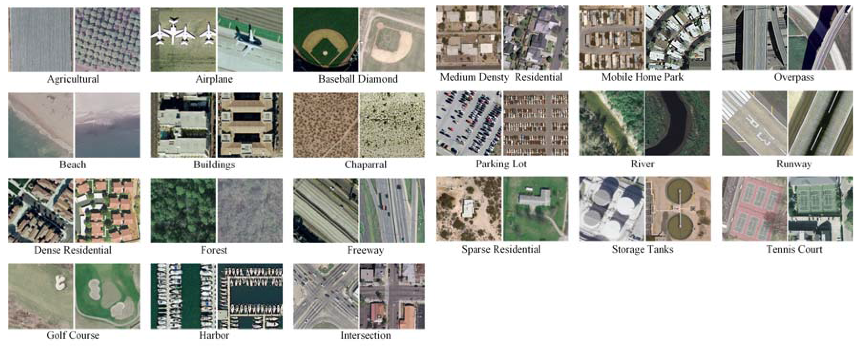
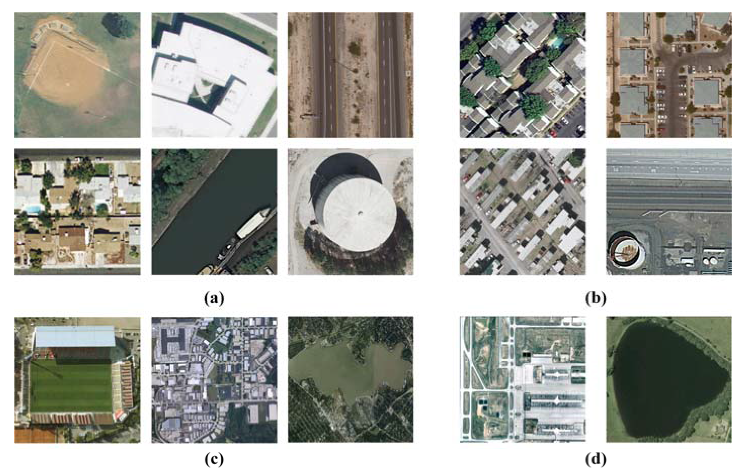
• UC Merced Land Use Dataset. The UC Merced dataset (UCM) is one of the first publicly available high-resolution remote sensing imagery data sets [4]. This dataset contains 21 typical land-use scene categories, each of which consists of 100 images measuring $256\times 256$ pixels with a pixel resolution of 30 cm in the red–green–blue color space. Figure 2 shows two examples of ground truth images from each class in this dataset. The classification of UCM dataset is challenging because of the high inter-class similarity among categories such as medium residential and dense residential areas.
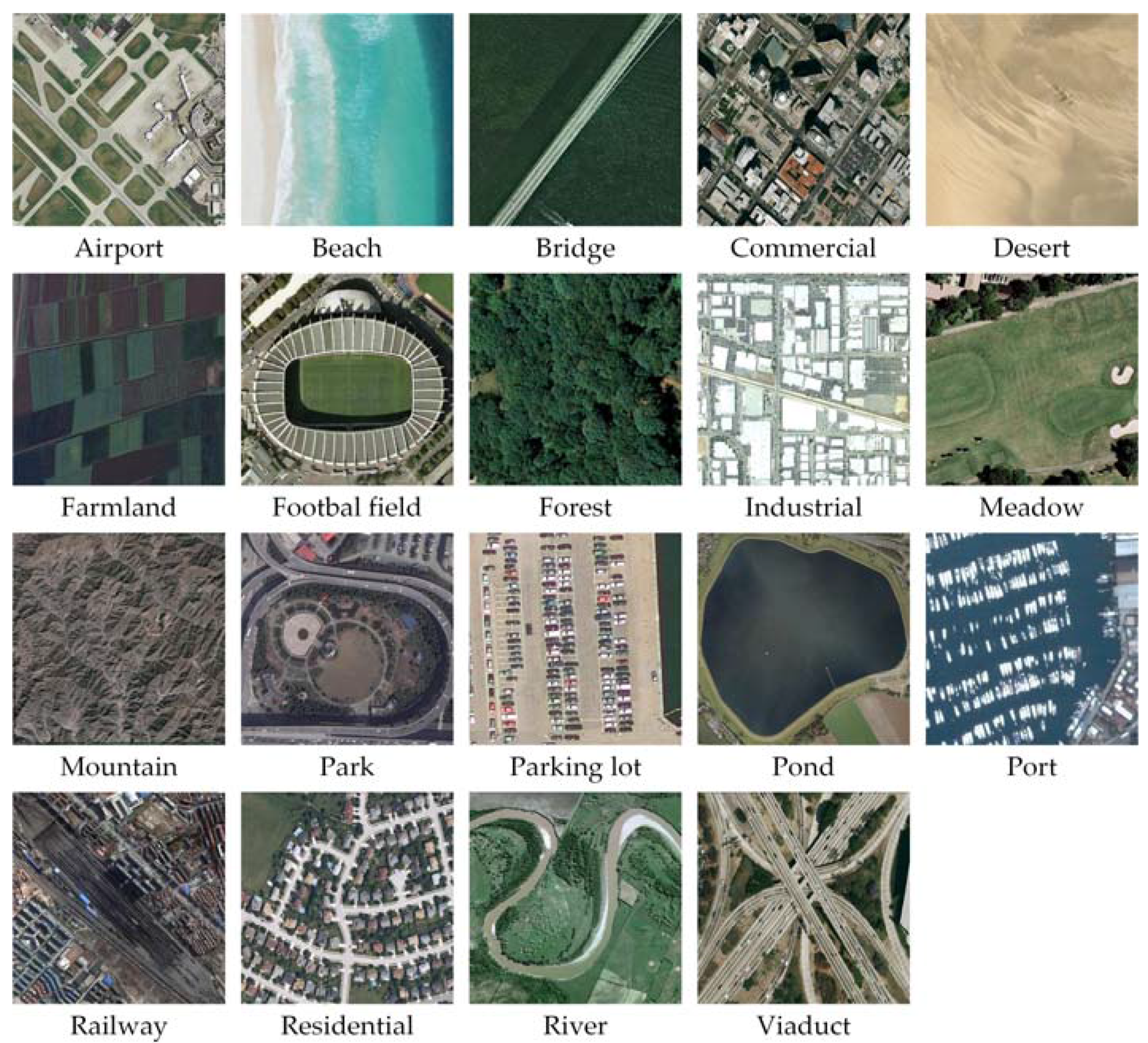
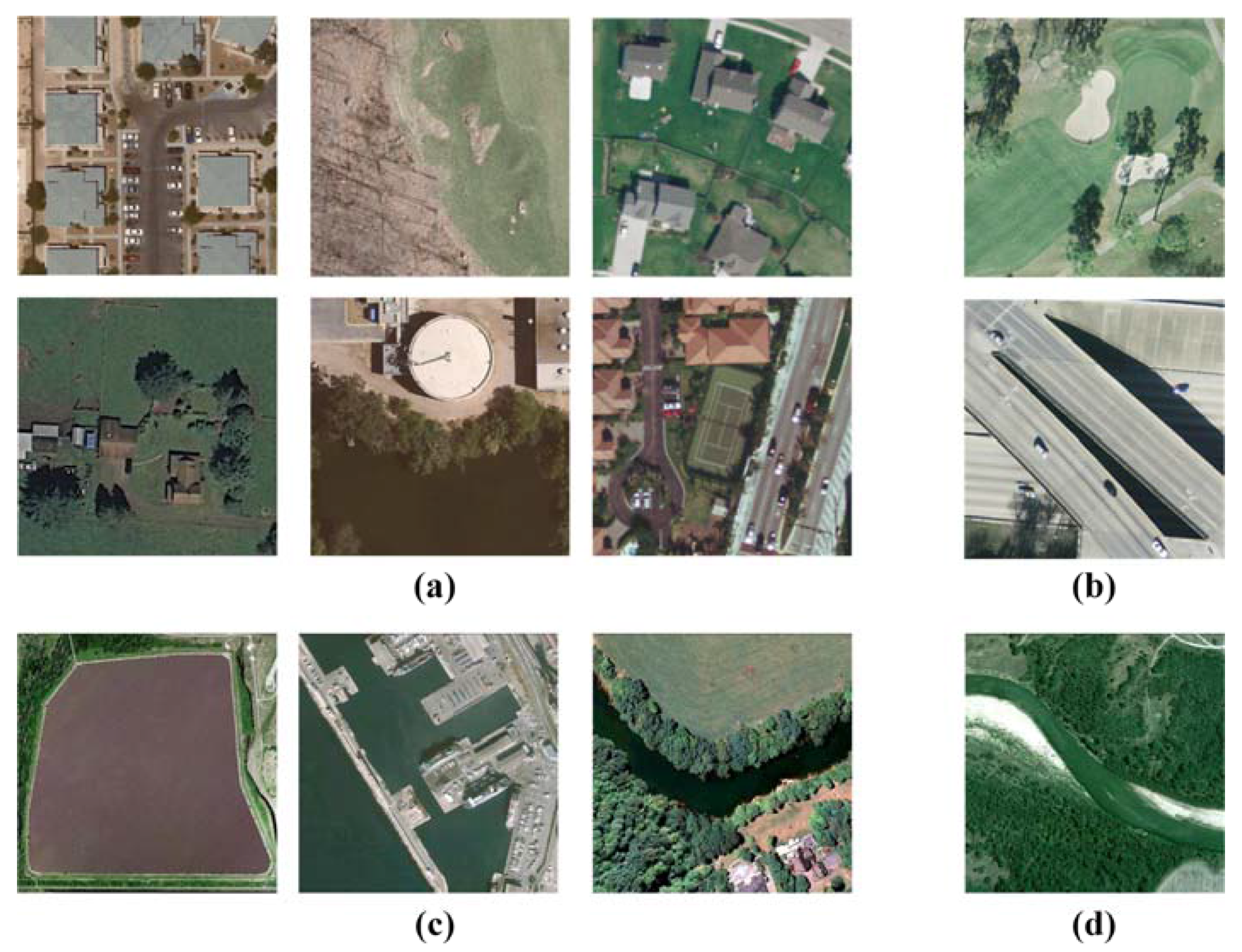
• WHU-RS Dataset. The WHU-RS dataset is a publicly available dataset in which all the images are collected from Google Earth (Google Inc., Mountain View, CA, USA) [5]. This dataset consists of 950 images with a size of $600\times 600$ pixels distributed among 19 scene classes. Examples of ground truth images are shown in Figure 3. As compared to the UCM dataset, the scene categories in the WHU-RS dataset are more complicated due to the variation in scale, resolution, and viewpoint-dependent appearance.

We randomly selected samples of each class for training the linear SVM classifier and the rest for testing. The sampling setting as in [48] are: 80 training samples per class for the UCM dataset and 30 training samples per class for the WHU-RS dataset. These two datasets were divided 50 times, each run with randomly selected training and testing samples, to obtain reliable results. The classification accuracy rate for categories were recorded as the mean and standard deviation of 50 runs. The public LIBLINEAR library [49] was used for SVM training and testing with linear kernel. We used 1-vs-rest SVM classifier, and the descriptors were $L_2$ normalized prior to learning. The exact choice of C had a negligible effect on performance after data normalization, so we set the learning constant to $C=1$. We also used the open source library VLFeat [50] for implementing the feature coding methods and MatConvNet [51] for extracting CNN features. The pre-trained CNN models used in this paper are available in the MatConvNet Pretrained Models [52]. In this paper, we used the VGG-M model to extract dense convolutional features. Experiments in this work were implemented using MathWorks Matlab 8.0, and were performed on the Microsoft Windows 10 operating system with a 3.3GHz quad-core Intel Xeon E3-1226 v3 CPU and a 2GB NVIDIA Quadro K620 GPU.

3.2. Parameter Sensitivity Analysis

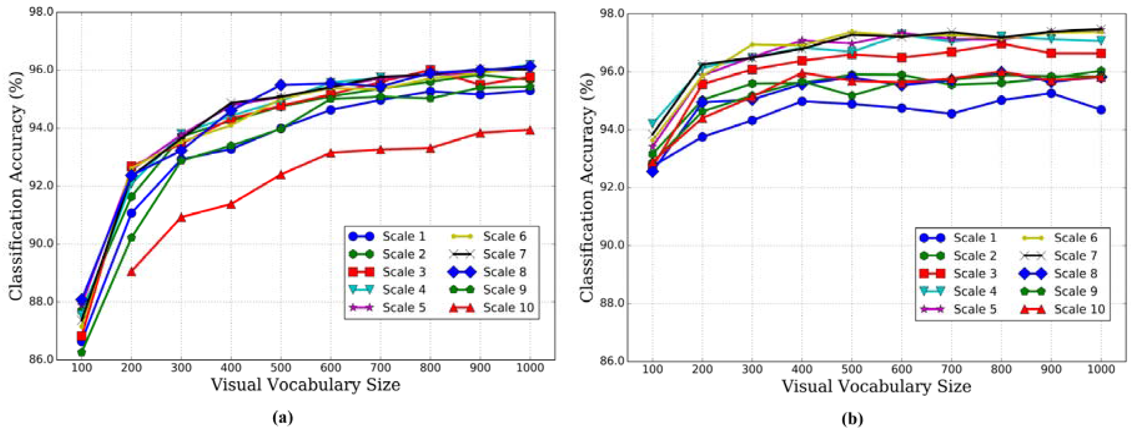
3.2.1. Effect of Multiscale Strategy

In the HRS images, objects show great variations in sizes and shapes. Accordingly, observation scale has a great impact on the land-use scene representations and classification accuracies. In this paper, we apply the multiscale strategy in the traditional correlaton framework to capture the spatial information at different scales. To measure the performance of MDDC with different number of scales, ten multiscale strategies were tested. As shown in

Table 1. The details of multiscale strategies.

Name	Values	Name	Values
Scale 1	1	Scale 6	$1,2^{-0.5},\dots ,2^{-2.0},2^{-2.5}$
Scale 2	$1,2^{-0.5}$	Scale 7	$1,2^{-0.5},\dots ,2^{-2.5},2^{-3.0}$
Scale 3	$1,2^{-0.5},2^{-1}$	Scale 8	$2^{0.5},1,\dots ,2^{-2.5},2^{-3.0}$
Scale 4	$1,2^{-0.5},2^{-1},2^{-1.5}$	Scale 9	$2^1,2^{0.5},\dots ,2^{-2.5},2^{-3.0}$
Scale 5	$1,2^{-0.5},2^{-1},2^{-1.5},2^{-2.0}$	Scale 10	$2^{1.5},1,\dots ,2^{-2.5},2^{-3.0}$

, we list the details of these strategies and give them names for convenient notation.

Land-use scene classification accuracies are affected by the number of visual words. Intuitively, histogram features lose discriminant capability if the visual vocabulary size is too small, and histograms from images of same class will never match if the visual vocabulary size is too large. Thus, we investigated effects of multiscale strategies and visual vocabulary sizes on the classification accuracy. We set the different sizes of visual vocabulary to 100, 200, 300, 400, 500, 600, 700, 800, 900 and 1000 on the UCM and WHU-RS datasets.

We evaluated effects of the visual vocabulary size and multiscale strategy on the appearance-based model, which used only histograms of visual words in the MDDC-based model. This is because the classification accuracies of the MDDC are determined by histograms of visual words and slightly improved by combining it with histograms of multiscale correlatons. As shown in Figure 4, the classification accuracies improved gradually with an increase in the number of visual words and up to a relative saturation point at each multiscale strategy. Most of the multiscale strategies improved classification accuracies, but multiscale strategies including supersampling may restrict effectiveness of the representation, and moreover might even be inferior to the single-scale strategy, such as “Scale 10” in Figure 4a. Generally, higher classification accuracies were achieved when more subsampling scales were used. However, the more scales used, the more memory consumption and computing time required. Accordingly, the “Scale 4” and “Scale 5” multiscale strategies were respectively adopted for the UCM and WHU-RS datasets during our experiments.

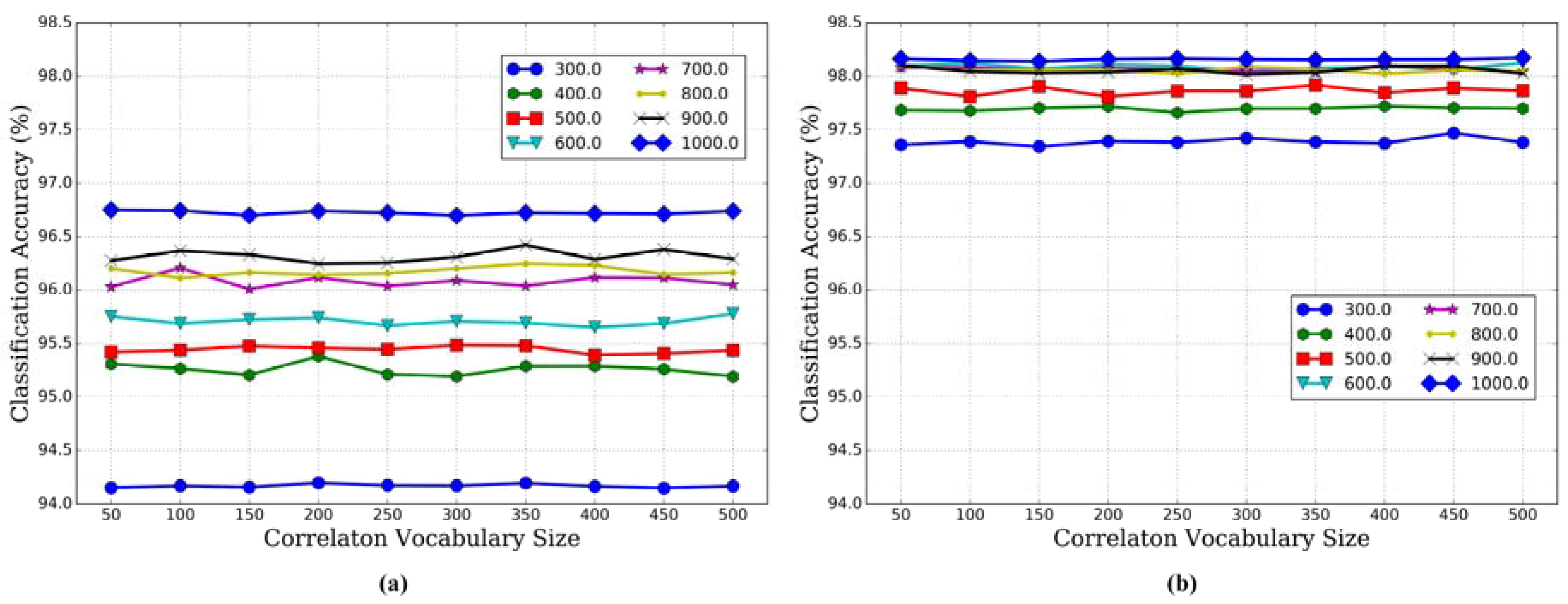
3.2.2. Effect of Correlaton Vocabulary Size

The multiscale correlaton vocabulary size can determine the effectiveness of spatial features. The effects of correlaton vocabulary sizes with different visual vocabulary sizes were tested for our MDDC model. We set the different sizes of correlaton vocabulary to 50, 100, 150, 200, 250, 300, 350, 400, 450 and 500, and the different sizes of visual vocabulary to 300, 400, 500, 600, 700, 800, 900 and 1000 in this experiment. Figure 5 shows the classification accuracy variation for the UCM and WHU-RS datasets using different correlaton vocabulary sizes with different visual vocabulary sizes. The plots hint that there is an obscure spot where classification accuracy is maximum and the size of correlaton vocabulary is optimal. This suggests that classification performance is not very sensitive to the size of correlaton vocabulary. Furthermore, the impact of visual vocabulary sizes on classification accuracy is far greater than the correlaton vocabulary size. Thus, we selected large visual vocabulary and small correlaton vocabulary, and set them to 1000 and 50 for the UCM and WHU-RS datasets.

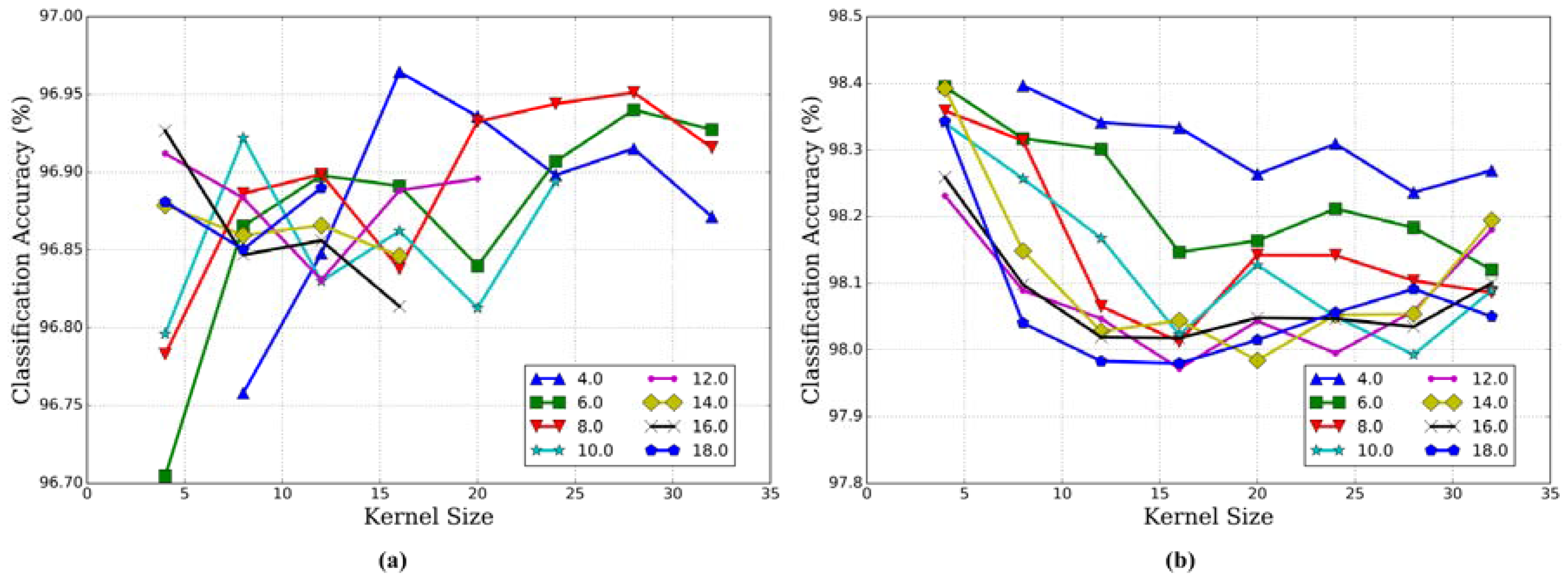
3.2.3. Kernel Size and Kernel Number

In the HRS images, land-use scenes show great variation in shape and scale, thus the size and number of kernels are critical to effective representation of complex land-use scenes. To quantitatively evaluate the effects of kernel sizes and kernel numbers on the classification accuracy, we tested different kernel numbers from 4 to 18 at interval of 2 and kernel sizes 4 to 32 at interval of 4. In addition, the maximum kernel radius, product of the kernel number and kernel size, was limited to the width/height of images, since larger kernel radius is unrelated to the accuracy. In these experiments, the sizes of visual vocabulary and correlaton vocabulary were respectively 1000 and 50 for both the UCM and WHU-RS datasets. The results of the MDDC-based model as a function of kernel size under different kernel numbers for these two datasets are reported in Figure 6.

The plot in Figure 6 indicates that the performance for each kernel size varied with kernel numbers on these two datasets. Generally, small kernel number has relatively high classification accuracies. One possible reason is that the land-use scenes in HRS images are deformable, so the spatial relationship among visual words is not very strict. Thus, a small number of kernels was sufficient to describe the spatial arrangement of visual words for these two datasets. Accordingly, we set the number of kernels to 4 for these two datasets in this study. For the UCM dataset, the classification accuracy on each kernel number generally increases with the kernel size and decreases after reaching the highest point; for the WHU-RS dataset, the classification accuracy for each kernel number generally decreases with the kernel size. This is because the scene categories in the WHU-RS dataset are more complicated, and hence the spatial correlation of visual words is more local and a smaller kernel size is more suitable. Therefore, we set the kernel size to 16 and 8 respectively for these two datasets in this study.

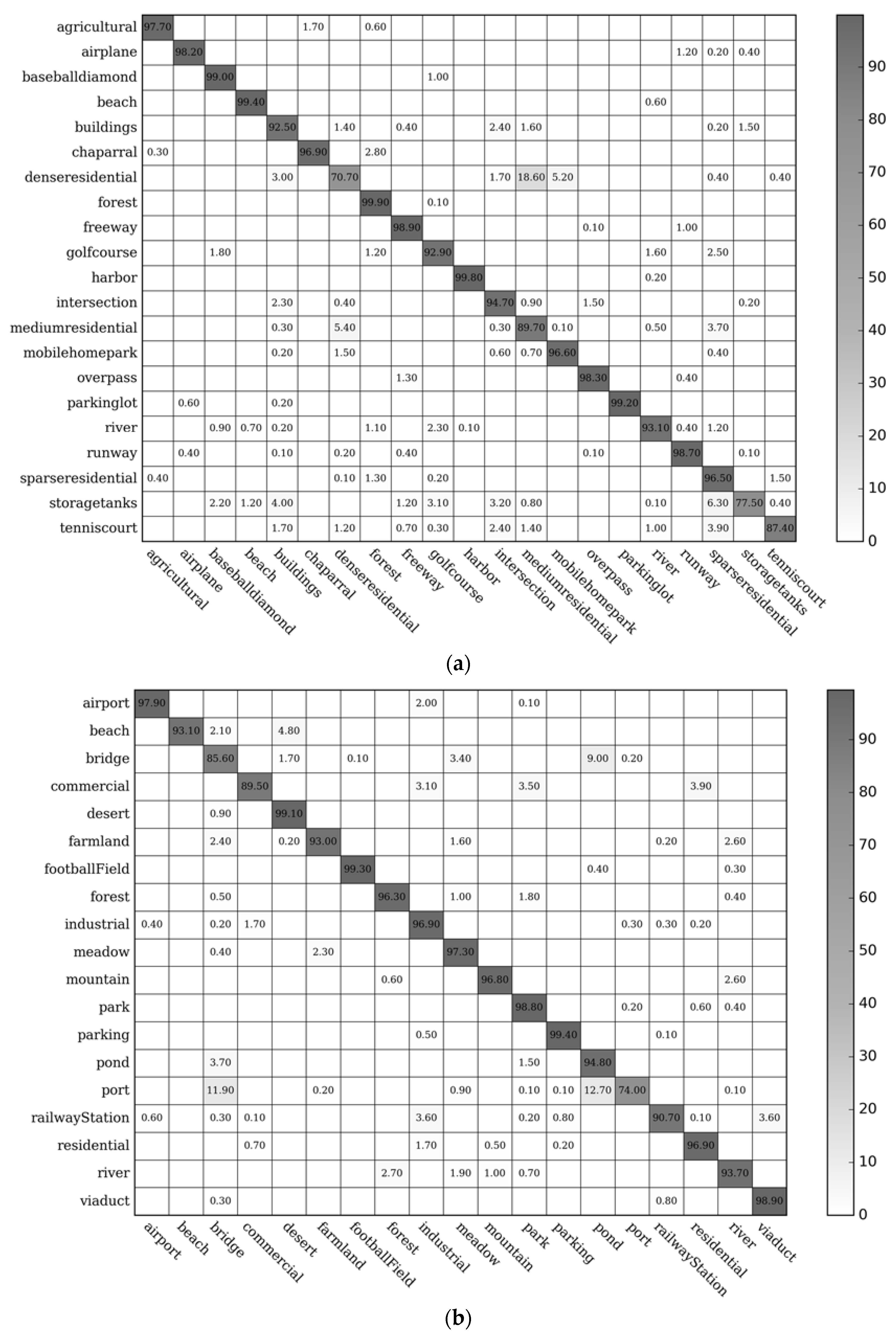
3.3. Confusion Matrix

The classification accuracies (%) of the individual classes on the UCM and WHU-RS datasets using the MDDC with parameters as previously described are shown in Figure 7. As shown in these confusion matrices, our proposed method can extract meaningful information for different categories in these two datasets. In Figure 7, there are 17 among 21 UCM land-use classes that have classification accuracies exceeding 90%; the classification accuracies of the baseball diamond, beach, forest, harbor and parking lot can reach 99%. For the WHU-RS dataset, classification values of 12 among 19 land-use categories were over 95%; especially, classification accuracies of the desert, football field, and parking can surpass 99%.

However, the similar categories, such as dense residential and medium residential areas in the UCM dataset and port and pond in the WHU-RS dataset, are very similar and intuitively hard to distinguish. From Figure 7, we find that diagonal values for baseball diamond, beach, forest, harbor and parking lot in the UCM dataset, and desert, football field, parking and viaduct in the WHU-RS dataset are extremely large; but diagonal values for dense residential area and storage tank in the UCM dataset, and port in the WHU-RS dataset relatively small. This is because categories with high performance possess rich texture and spatial layout information, and the within-class similarity of them is high; categories with poor performance have relatively low with-in similarity, and some images in these categories are easily confused with other classes, i.e., dense residential and medium residential areas in the UCM dataset.

3.4. Comparison with State-of-the-Art Methods

To illustrate the effectiveness of the MDDC-based model, we compared our results with various state-of-the-art methods that have reported classification accuracies on the UCM dataset. As shown in

Table 2. Comparison of classification accuracy (%) on the UCM dataset.

Method	Accuracy (Mean ± Std)
BoVW [15]	71.86
SPM [19]	74.0
SPCK++ [4]	77.38
MS-based Correlaton [20]	81.32 ± 0.92
UFL [7]	81.67 ± 1.23
SG + UFL [8]	82.72 ± 1.18
UFL-SC [10]	90.26 ± 1.51
UFC + MSC [11]	91.95 ± 0.72
CCM-BoVW [21]	86.64 ± 0.81
PSR [22]	89.1
MSIFT [6]	90.97 ± 1.81
MS-CLBP + FV [56]	93.0 ± 1.2
MTJSLRC [55]	91.07 ± 0.67
VLAT [57]	94.3
MBVW [25]	96.14
OverFeat [31]	90.91 ± 1.19
CaffeNet [31]	93.42 ± 1.0
GoogLeNet + Fine-tune [53]	97.1
Appearance-based	96.05 ± 0.62
MDDC	96.92 ± 0.57

, our MDDC method largely outperforms methods that use a sophisticated learning strategy with low-level hand-engineered feature and non-linear classifiers, such as these SIFT-based BoVW and its extension forms like SPM [19] and Spatial Pyramid Co-occurrence Kernel (SPCK++) [4]. Furthermore, Unsupervised Feature Learning methods (UFLs) [7], and their Saliency-Guided version SG + UFL [8] and Spectral Clustering version UFL-SC [10] were also involved in the comparison.

The results show that our proposed method outperforms all these methods except for the well-designed deep learning framework, GoogleLeNet + Fine-tune approach [53], in terms of classification accuracy. However, our proposed method extracts CNN activations without changing the parameters of the pre-trained CNN, whereas the GoogleLeNet + Fine-tune approach fine tunes the pre-trained CNN (GoogLeNet [54]) on the target dataset. The comparison results indicate that our MDDC-based model using deeply described visual words at multiple scales has great potential for the representation of land-use scene images.

The comparison results on the WHU-RS dataset are listed in

Table 3. Comparison of classification accuracy (%) on the WHU-RS dataset.

Method	Accuracy (Mean ± Std)
Bag of SIFT [58]	85.5 ± 1.2
LTP-HF [59]	77.6
MS-CLBP [59]	93.4 ± 1.1
Multi-feature Concatenation [58]	90.8 ± 0.7
MTJSLRC [55]	91.74 ± 1.14
SIFT + LTP-HF + Color Histogram [48]	93.6
MS-CLBP + FV [56]	94.32 ± 1.2
Appearance-based	97.34 ± 0.57
MDDC	98.27 ± 0.53

. It presents that the MDDC outperforms these previously proposed methods. Our proposed method achieved about 6.53% improvement over the MTJSLRC method [55] which utilized a combination of multiple sets of features. Overall, the remarkable classification results achieved on these public benchmarks indicate the superior discriminative capability of the proposed feature representation for the land-use scene. Furthermore, the MDDC-based model provides a path to connect the mid-level deeply described visual words and the semantics of land-use scenes considering the spatial information at multiple scales with relatively low computational complexity; and we can process any image size by convolutional layers and avoid costly resizing operations.

4. Discussion

Extensive experiments show that our MDDC-based model, which integrates the deep learning framework with the correlaton method, is very effective for land-use scene classification in HRS images. The co-occurrence of visual words at different scales is captured in a discriminative visual representation. Hence, the proposed model can integrate appearance and spatial information jointly at different scales, and effectively represent the land-use scene images. Experimental results on the UCM and WHU-RS datasets indicate that the proposed model is competitive with the state-of-the-art methods for land-use scene classification.

To discriminate these land-use classes, traditional correlaton methods were applied to explore the appearance and spatial features on a single-scale image. However, objects in HRS images tend to appear at various scales. The MDDC first transforms the original image into several images at different scales, and then uses these multiscale images to extract multiscale dense convolutional features. We flatten these features into vectors for multiscale deeply described visual word generation. The effectiveness of multiscale strategies is demonstrated in Section 3.2.1. Several example images are presented in Figure 8 that compare results from the single-scale and multiscale appearance-based model on the UCM and WHU-RS datasets.

As shown in Figure 8, these land-use images covering objects of large scale, like the building and storage tank in Figure 8a, can be recognized by the multiscale appearance-based model. Due to more information in the multiscale representation, the multiscale model is more robust with respect to clutter background, like the industrial area and pond in Figure 8c, but, some land-use images containing small objects are failed by the multiscale model. For example, the storage tank in Figure 8b was recognized incorrectly as freeway. This is because features of the storage tank in this image became insignificant, whereas features of the road were more dominant under multiple scales especially with the subsampling of images. In the multiscale appearance-based model, land-use categories covering similar objects yet varying density are probably difficult to distinguish, such as the dense and medium residential categories in Figure 8b. Overall, the multiscale model raised classification accuracies by approximately 0.89% and 2.21% respectively for the UCM and WHU-RS datasets. The improvement of classification accuracy on the WHU-RS dataset is more significant because of variation in scale and resolution of images in this dataset.

To incorporate appearance and shape information jointly in multiple scales, we produced correlograms using labels of visual words at different scales. Multiscale correlatons were generated by an adaptive vector quantization of multiscale correlograms to achieve a compact spatial representation without loss of discrimination. There are some examples where multiscale appearance-based model failed but the MDDC-based model worked well in Figure 9.

As shown in Figure 9, the MDDC-based model can recognize land-use scenes covering clutter background and objects with broad or intrinsic structure. This indicates that representations based on histograms of multiscale correlatons can capture shape information across object classes. However, categories with resemble shape can easily get confused, such as the overpass image in Figure 9b was recognized incorrectly as freeway category. Altogether, the MDDC-based model improved classification accuracies by approximately 0.87% and 0.93% respectively for the UCM and WHU-RS datasets.

These experimental results demonstrate that features extracted from pre-trained CNN using large natural image datasets have stronger representative ability than low-level hand-crafted features, and generalize well to HRS image datasets. Classification results using multiscale features delivered better performance than the single-scale features. By capturing the co-occurrence of visual words at different scales in a discriminative visual representation, the MDDC can improve classification accuracies. This MDDC-based representation of joint appearance and spatial information at multiple scales yielded good performance results using a simple linear classifier.

5. Conclusions

In this paper, a multiscale deeply described correlaton method was presented to extract appearance and spatial features for land-use scene classification in HRS images. This method constructs multiscale dense convolutional features by subsampling original HRS images; encodes the multiscale deeply described visual words using the output of the last convolutional layer in a pre-trained CNN. The co-occurrence of deeply described visual words is captured by correlograms at different scales. The major contribution of this paper is that the traditional correlaton method was extended to MDDC for learning spatial features at multiple scales. The MDDC-based model is evaluated using two publicly available ground truth image datasets. The experimental results prove that the proposed method delivers competitive performance in classification accuracy against the state-of-the-art methods. In future studies, we plan to investigate a spatial pooling strategy inspired by the correlaton model to directly learn the optimal parameters, such as the kernel number and kernel size, for different land-use scene categories.

References

1. Zhou, W.; Troy, A. An object-oriented approach for analysing and characterizing urban landscape at the parcel level. Int. J. Remote Sens. 2008, 29, 3119–3135. [Google Scholar] [CrossRef]
2. Zhang, H.; Lin, H.; Li, Y.; Zhang, Y. Feature extraction for high-resolution imagery based on human visual perception. Int. J. Remote Sens. 2013, 34, 1146–1163. [Google Scholar] [CrossRef]
3. Rogan, J.; Chen, D. Remote sensing technology for mapping and monitoring land-cover and land-use change. Prog. Plan. 2004, 61, 301–325. [Google Scholar] [CrossRef]
4. Yang, Y.; Newsam, S. Bag-of-visual-words and spatial extensions for land-use classification. In Proceedings of the 18th SIGSPATIAL International Conference on Advances in Geographic Information Systems, San Jose, CA, USA, 2–5 November 2010; pp. 270–279. [Google Scholar]
5. Xia, G.S.; Yang, W.; Delon, J.; Gousseau, Y.; Sun, H.; Maitre, H. Structrual high-resolution satellite image indexing. In Proceedings of the ISPRS, TC VII Symposium Part A: 100 Years ISPRS—Advancing Remote Sensing Science, Vienna, Austria, 5–7 July 2010. [Google Scholar]
6. Cheng, G.; Han, J.; Zhou, P.; Guo, L. Multi-class geospatial object detection and geographic image classification based on collection of part detectors. ISPRS J. Photogramm. Remote Sens. 2014, 98, 119–132. [Google Scholar] [CrossRef]
7. Cheriyadat, A. Unsupervised feature learning for aerial scene classification. IEEE Trans. Geosci. Remote Sens. 2014, 52, 439–451. [Google Scholar] [CrossRef]
8. Zhang, F.; Du, B.; Zhang, L. Saliency-guided unsupervised feature learning for scene classification. IEEE Trans. Geosci. Remote Sens. 2015, 53, 2175–2184. [Google Scholar] [CrossRef]
9. Fan, J.; Tan, H.L.; Lu, S. Multipath sparse coding for scene classification in very high resolution satellite imagery. SPIE Remote Sens. 2015, 9643, 96430S. [Google Scholar]
10. Hu, F.; Xia, G.; Wang, Z.; Huang, X.; Zhang, L.; Sun, H. Unsupervised feature learning via spectral clustering of multidimensional patches for remotely sensed scene classification. IEEE J. Sel. Top. Appl. Earth Obs. Remote Sens. 2015, 8, 2015–2030. [Google Scholar] [CrossRef]
11. Fan, J.; Chen, T.; Lu, S. Unsupervised feature learning for land-use scene recognition. IEEE Trans. Geosci. Remote Sens. 2017, 55, 2250–2261. [Google Scholar] [CrossRef]
12. Chehdi, K.; Soltani, M.; Cariou, C. Pixel classification of large-size hyperspectral images by affinity propagation. J. Appl. Remote Sens. 2014, 8, 083567. [Google Scholar] [CrossRef]
13. Yu, Q. Object-based detailed vegetation classification with airborne high spatial resolution remote sensing imagery. Photogramm. Eng. Remote Sens. 2006, 72, 799–811. [Google Scholar] [CrossRef]
14. Zhao, Y.; Zhang, L.; Li, P.; Huang, B. Classification of high spatial resolution imagery using improved gaussian markov random-field-based texture features. IEEE Trans. Geosci. Remote Sens. 2007, 45, 1458–1468. [Google Scholar] [CrossRef]
15. Sivic, J.; Zisserman, A. Video Google: A text retrieval approach to object matching in videos. In Proceedings of the IEEE International Conference on Computer Vision, Nice, France, 13–16 October 2003; pp. 1470–1477. [Google Scholar]
16. Csurka, G.; Dance, C.R.; Fan, L.; Willamowski, J.; Bray, C. Visual categorization with bags of keypoints. In Proceedings of the Workshop on Statistical Learning in Computer Vision, European Conference on Computer Vision, Prague, Czech Republic, 11–14 May 2004; pp. 1–22. [Google Scholar]
17. Bosch, A.; Zisserman, A.; Muoz, X. Scene classification using a hybrid generative/discriminative approach. IEEE Trans. Pattern Anal. Mach. Intell. 2008, 30, 712–727. [Google Scholar] [CrossRef] [PubMed]
18. Jegou, H.; Douze, M.; Schmid, C. Improving bag-of-features for large scale image search. Int. J. Comput. Vis. 2010, 87, 316–336. [Google Scholar] [CrossRef] [Green Version]
19. Lazebnik, S.; Schmid, C.; Ponce, J. Beyond bags of features: Spatial pyramid matching for recognizing natural scene categories. In Proceedings of the IEEE Conference on Computer Vision and Pattern Recognition, New York, NY, USA, 17–22 June 2006; pp. 2169–2178. [Google Scholar]
20. Qi, K.; Wu, H.; Shen, C.; Gong, J. Land-use scene classification in high-resolution remote sensing images using improved correlatons. IEEE Geosci. Remote Sens. Lett. 2015, 12, 2403–2407. [Google Scholar] [CrossRef]
21. Zhao, L.J.; Tang, P.; Huo, L.Z. Land-use scene classification using a concentric circle-structured multiscale bag-of-visual-words model. IEEE J. Sel. Top. Appl. Earth Obs. Remote Sens. 2014, 7, 4620–4631. [Google Scholar] [CrossRef]
22. Chen, S.; Tian, Y. Pyramid of spatial relations for scene-level land use classification. IEEE Trans. Geosci. Remote Sens. 2015, 53, 1947–1957. [Google Scholar] [CrossRef]
23. Lowe, D.G. Distinctive image features from scale-invariant keypoints. Int. J. Comput. Vis. 2004, 60, 91–110. [Google Scholar] [CrossRef]
24. Dalal, N.; Triggs, B. Histograms of oriented gradients for human detection. In Proceedings of the IEEE Computer Society Conference on Computer Vision and Pattern Recognition, San Diego, CA, USA, 25–25 June 2005; pp. 886–893. [Google Scholar]
25. Zhao, W.; Du, S. Scene classification using multi-scale deeply described visual words. Int. J. Remote Sens. 2016, 37, 4119–4131. [Google Scholar] [CrossRef]
26. Krizhevsky, A.; Sutskever, I.; Hinton, G.E. Imagenet classification with deep convolutional neural networks. In Proceedings of the Twenty-Sixth Annual Conference on Neural Information Processing Systems, Lake Tahoe, NY, USA, 3–8 December 2012; pp. 1097–1105. [Google Scholar]
27. Girshick, R.; Donahue, J.; Darrell, T.; Malik, J. Rich feature hierarchies for accurate object detection and semantic segmentation. In Proceedings of the IEEE Conference on Computer Vision and Pattern Recognition, Columbus, OH, USA, 23–28 June 2014; pp. 580–587. [Google Scholar]
28. Hariharan, B.; Arbelaez, P.; Girshick, R.; Malik, J. Simultaneous detection and segmentation. In Proceedings of the European Conference on Computer Vision, Zurich, Switzerland, 6–12 September 2014; pp. 297–312. [Google Scholar]
29. Cheng, G.; Han, J.; Lu, X. Remote sensing image scene classification: Benchmark and state of the art. Proc. IEEE 2017, 1–19. [Google Scholar] [CrossRef]
30. Cimpoi, M.; Maji, S.; Kokkinos, I.; Vedaldi, A. Deep filter banks for texture recognition, description, and segmentation. Int. J. Comput. Vis. 2016, 118, 65–94. [Google Scholar] [CrossRef] [PubMed]
31. Penatti, O.A.; Nogueira, K.; dos Santos, J.A. Do deep features generalize from everyday objects to remote sensing and aerial scenes domains? In Proceedings of the IEEE Conference on Computer Vision and Pattern Recognition Workshops, Boston, MA, USA, 12 June 2015; pp. 44–51. [Google Scholar]
32. Chatfield, K.; Simonyan, K.; Vedaldi, A.; Zisserman, A. Return of the devil in the details: Delving deep into convolutional nets. In Proceedings of the British Machine Vision Conference, Nottingham, UK, 1–5 September 2014. [Google Scholar]
33. Donahue, J.; Jia, Y.; Vinyals, O.; Hoffman, J.; Zhang, N.; Tzeng, E.; Darrell, T. DeCAF: A deep convolutional activation feature for generic visual recognition. In Proceedings of the International Conference on Machine Learning, Beijing, China, 21–26 June 2014; pp. 647–655. [Google Scholar]
34. Oquab, M.; Bottou, L.; Laptev, I.; Sivic, J. Learning and transferring mid-level image representations using convolutional neural networks. In Proceedings of the IEEE Conference on Computer Vision and Pattern Recognition, Columbus, OH, USA, 23–28 June 2014; pp. 1717–1724. [Google Scholar]
35. Zeiler, M.D.; Fergus, R. Visualizing and understanding convolutional networks. In Proceedings of the European Conference on Computer Vision, Zurich, Switzerland, 6–12 September 2014; pp. 818–833. [Google Scholar]
36. Hu, F.; Xia, G.; Hu, J.; Zhang, L. Transferring deep convolutional neural networks for the scene classification of high-resolution remote sensing imagery. Remote Sens. 2015, 7, 14680–14707. [Google Scholar] [CrossRef]
37. Deng, J.; Dong, W.; Socher, R.; Li, L.J.; Li, K.; Fei-Fei, L. Imagenet: A large-scale hierarchical image database. In Proceedings of the IEEE Conference on Computer Vision and Pattern Recognition, Miami, FL, USA, 20–25 June 2009; pp. 248–255. [Google Scholar]
38. Grauman, K.; Darrell, T. The pyramid match kernel: Discriminative classification with sets of image features. In Proceedings of the International Conference on Computer Vision, Beijing, China, 17–21 October 2005; pp. 1458–1465. [Google Scholar]
39. He, K.; Zhang, X.; Ren, S.; Sun, J. Spatial pyramid pooling in deep convolutional networks for visual recognition. IEEE Trans. Pattern Anal. Mach. Intell. 2015, 37, 1904–1916. [Google Scholar] [CrossRef] [PubMed]
40. Lu, X.; Zheng, X.; Yuan, Y. Remote sensing scene classification by unsupervised representation learning. IEEE Trans. Geosci. Remote Sens. 2017, 55, 1–10. [Google Scholar] [CrossRef]
41. Battiato, S.; Farinella, G.M.; Gallo, G.; Ravi, D. Spatial hierarchy of textons distributions for scene classification. In Proceedings of the Conference on Multimedia Modeling, Sophia Antipolis, France, 7–9 January 2009; pp. 333–343. [Google Scholar]
42. Zhou, L.; Zhou, Z.; Hu, D. Scene classification using multi-resolution low-level feature combination. Neurocomputing 2013, 122, 284–297. [Google Scholar] [CrossRef]
43. Huang, J.; Kumar, S.R.; Mitra, M.; Zhu, W.; Zabih, R. Image indexing using color correlograms. In Proceedings of the IEEE Conference on Computer Vision and Pattern Recognition, San Juan, Puerto Rico, 17–18 June 1997; pp. 762–768. [Google Scholar]
44. Savarese, S.; Winn, J.; Criminisi, A. Discriminative object class models of appearance and shape by correlatons. In Proceedings of the IEEE Conference on Computer Vision and Pattern Recognition, Washington, DC, USA, 17–22 June 2006; pp. 2033–2040. [Google Scholar]
45. Fukushima, K. Neocognitron: A self-organizing neural network model for a mechanism of pattern recognition unaffected by shift in position. Biol. Cybern. 1980, 36, 193–202. [Google Scholar] [CrossRef] [PubMed]
46. LeCun, Y.; Bottou, L.; Bengio, Y.; Haffner, P. Gradient-based learning applied to document recognition. Proc. IEEE 1998, 86, 2278–2324. [Google Scholar] [CrossRef]
47. Qi, K.; Zhang, X.; Wu, B.; Wu, H. Sparse coding-based correlaton model for land-use scene classification in high-resolution remote-sensing images. J. Appl. Remote Sens. 2016, 10, 042005. [Google Scholar]
48. Sheng, G.; Yang, W.; Xu, T.; Sun, H. High-resolution satellite scene classification using a sparse coding based multiple feature combination. Int. J. Remote Sens. 2012, 33, 2395–2412. [Google Scholar] [CrossRef]
49. Fan, R.E.; Chang, K.W.; Hsieh, C.J.; Wang, X.R.; Lin, C.J. LIBLINEAR: A library for large linear classification. J. Mach. Learn. Res. 2008, 9, 1871–1874. [Google Scholar]
50. Vedaldi, A.; Fulkerson, B. VLFeat: An open and portable library of computer vision algorithms. Available online: http://www.vlfeat.org/ (accessed on 16 November 2016).
51. Vedaldi, A.; Lenc, K. MatConvNet: CNNs for MATLAB. Available online: http://www.vlfeat.org/matconvnet (accessed on 16 November 2016).
52. MatConvNet Pretrained Models. Available online: http://www.vlfeat.org/matconvnet/pretrained/ (accessed on 16 November 2016).
53. Castelluccio, M.; Poggi, G.; Sansone, C.; Verdoliva, L. Land Use Classification in Remote Sensing Images by Convolutional Neural Networks. Available online: http://arxiv.org/abs/1508.00092 (accessed on 30 March 2017).
54. Gong, Y.; Wang, L.; Guo, R.; Lazebnik, S. Multi-scale orderless pooling of deep convolutional activation features. In Proceedings of the European Conference on Computer Vision, Zurich, Switzerland, 6–12 September 2014; pp. 392–407. [Google Scholar]
55. Qi, K.; Liu, W.; Yang, C.; Guan, Q.; Wu, H. Multi-task joint sparse and low-rank representation for the scene classification of high-resolution remote sensing image. Remote Sens. 2017, 9, 10. [Google Scholar] [CrossRef]
56. Huang, L.; Chen, C.; Li, W.; Du, Q. Remote sensing image scene classification using multi-scale completed local binary patterns and fisher vectors. Remote Sens. 2016, 8, 483. [Google Scholar] [CrossRef]
57. Negrel, R.; Picard, D.; Gosselin, P.H. Evaluation of second-order visual features for land-use classification. In Proceedings of the International Workshop on Content-Based Multimedia Indexing, Klagenfurt, Austria, 18–20 June 2014; pp. 1–5. [Google Scholar]
58. Liu, C. Maximum likelihood estimation from incomplete data via EM-type Algorithms. In Advanced Medical Statistics; World Scientific Publishing Co.: Hackensack, NJ, USA, 2003; pp. 1051–1071. [Google Scholar]
59. Krapac, J.; Verbeek, J.; Jurie, F. Modeling spatial layout with fisher vectors for image categorization. In Proceedings of the International Conference on Computer Vision, Barcelona, Spain, 6–13 November 2011; pp. 1487–1494. [Google Scholar]
Figure 1. Flow chart of our MDDC model for land-use scene classification.
Remotesensing 09 00917 g001
Figure 2. Two example ground truth images of each scene category in the UCM dataset.
Remotesensing 09 00917 g002
Figure 3. Example ground truth images of each scene category in the WHU-RS dataset.
Remotesensing 09 00917 g003
Figure 4. Effects of scale strategies at different vocabulary size for the appearance-based model. (a) Effects on the UCM dataset; (b) Effects on the WHU-RS dataset. The details of these multiscale strategies are listed in Table 1.
Remotesensing 09 00917 g004
Figure 5. Performance variation using different correlaton vocabulary sizes with different visual vocabulary sizes for the MDDC (lines in figures represent different correlaton vocabulary sizes). (a) Performance on the UCM dataset; (b) Performance on the WHU-RS dataset.
Remotesensing 09 00917 g005
Figure 6. Classification accuracy of the MDDC-based model as a function of kernel size under different kernel numbers (lines in figures represent different kernel numbers). (a) The UCM dataset; (b) The WHU-RS dataset.
Remotesensing 09 00917 g006
Figure 7. Confusion matrices showing classification accuracies (%) for the proposed model. (a) Confusion matrix for the UCM dataset; (b) Confusion matrix for the WHU-RS dataset.
Remotesensing 09 00917 g007
Figure 8. Several example images that compare results from the single-scale and multiscale appearance-based models. Images where single-scale model failed are shown in (a) UCM and (c) WHU-RS; Images where multiscale model failed are shown in (b) UCM and (d) WHU-RS.
Remotesensing 09 00917 g008
Figure 9. Several example images that compare results from multiscale appearance-based and MDDC-based models. Images where multiscale appearance-based model failed are shown in (a) UCM and (c) WHU-RS; Images where the MDDC-based model failed are shown in (b) UCM and (d) WHU-RS.
Remotesensing 09 00917 g009