Estimating Ground Level NO₂ Concentrations over Central-Eastern China Using a Satellite-Based Geographically and Temporally Weighted Regression Model

Abstract

People in central-eastern China are suffering from severe air pollution of nitrogen oxides. Top-down approaches have been widely applied to estimate the ground concentrations of NO₂ based on satellite data. In this paper, a one-year dataset of tropospheric NO₂ columns from the Ozone Monitoring Instrument (OMI) together with ambient monitoring station measurements and meteorological data from May 2013 to April 2014, are used to estimate the ground level NO₂. The mean values of OMI tropospheric NO₂ columns show significant geographical and seasonal variation when the ambient monitoring stations record a certain range. Hence, a geographically and temporally weighted regression (GTWR) model is introduced to treat the spatio-temporal non-stationarities between tropospheric-columnar and ground level NO₂. Cross-validations demonstrate that the GTWR model outperforms the ordinary least squares (OLS), the geographically weighted regression (GWR), and the temporally weighted regression (TWR), produces the highest R² (0.60) and the lowest values of root mean square error mean (RMSE), absolute difference (MAD), and mean absolute percentage error (MAPE). Our method is better than or comparable to the chemistry transport model method. The satellite-estimated spatial distribution of ground NO₂ shows a reasonable spatial pattern, with high annual mean values (>40 μg/m³), mainly over southern Hebei, northern Henan, central Shandong, and southern Shaanxi. The values of population-weight NO₂ distinguish densely populated areas with high levels of human exposure from others.

1. Introduction

High ground level nitrogen oxides (NO_x = NO + NO₂) are identified to be deleterious to human health, including decreased lung function and an increased risk of respiratory symptoms [1,2]. In addition, NO_x can also produce other photochemical pollutants like O₃ in photochemical reactions, and acts as a gaseous precursor of aerosols and acid rain. Thus, the NO_x concentration has been included in multi-pollutant health indices [3] and its monitoring with complete spatial coverage is needed for exposure assessment. Since 1995, a series of satellites sensors, e.g., the Global Ozone Monitoring Experiment (GOME), the Scanning Imaging Absorption Spectrometer for Atmospheric Cartography (SCIAMACHY), and the Ozone Monitoring Instrument (OMI) have been successfully used to retrieve vertical NO₂ columns [4,5,6,7,8]. A dramatic increase in tropospheric NO₂ columns was revealed by the GOME and SCIAMACHY observations over China [9,10,11,12], the world’s largest developing country along with the fastest growing economy.

Given that the existing ambient monitoring stations are sparse and unevenly distributed, there is a growing interest in the top-down satellite approach to obtain timely map of the spatial variations of surface concentrations of NO₂. A close relationship between ground level NO₂ concentrations and satellite-retrieved tropospheric NO₂ columns is expected based on two facts: (1) ground level NO₂ accounts for the majority of tropospheric NO₂ columns since human activities are their main source; and (2) the short lifetime of near-surface NO₂ results in little transport, both vertically and horizontally [13]. Petritoli et al. [14] demonstrated a significant correlation between in situ NO₂ measurements and the GOME tropospheric NO₂ columns. Recently, satellite observations were combined with land use regression models to provide spatio-temporally resolved ambient NO₂ [15,16,17]. In addition, an approach proposed by Lamsal et al. [18] that combines the vertical profiles of NO₂ generated by the chemical transport model and satellite tropospheric NO₂ columns, has been widely used to estimate ground level NO₂ concentrations [19,20]. However, the emission inventories used for the model simulations are based on outdated statistical data about human activities. These model-based profiles may not capture the actual vertical distribution of NO₂, especially where anthropogenic NO_x emissions are undergoing rapid changes such as in China [21]. Kim et al. [22] estimated the surface NO₂ volume mixing ratio by using multiple regression models with OMI data.

In this study, a geographically and temporally weighted regression (GTWR) model is introduced to estimate the ground level NO₂ concentrations by using the OMI tropospheric NO₂ columns over central-eastern China. The GTWR model is adapted from the geographically weighted regression (GWR) model [23,24,25,26] by taking into account spatio-temporal non-stationarity, which has been proven to effectively establish the relation between satellite-retrieved aerosol optical depth and fine particulate matter (PM_2.5) [27,28]. Furthermore, population-weighted ground level NO₂ concentrations are calculated to evaluate population exposure levels in different regions.

2. Study Area and Data

2.1. Study Area

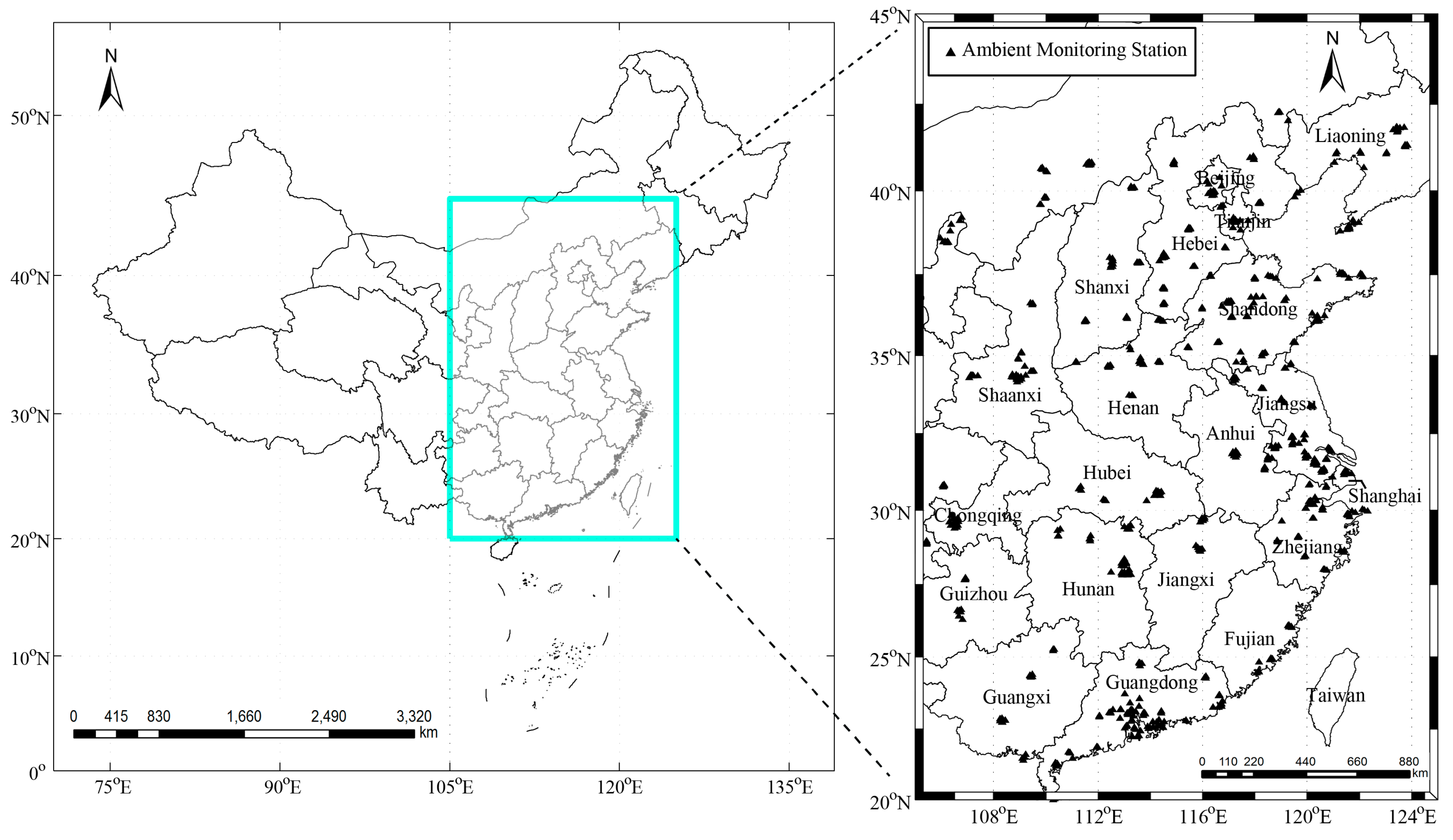
This study focuses on the central-eastern China with a geographic scope of 20°N–45°N and 105°E–124°E (major populated areas in China, see left panel in Figure 1). The study area covers 20 province-level administrative units in mainland China, including the regions of the North China Plain, Yangtze River Delta, and Pearl River Delta that are most polluted. 715 ambient monitoring stations are located in this study area (see the right panel in Figure 1).

2.2. OMI Tropospheric NO₂ Columns

OMI is a Dutch-Finnish nadir-viewing hyperspectral instrument onboard the Earth Observing System Aura satellite in a Sun-synchronous orbit with an equatorial crossing time of approximately 13:45 local time. It measures sunlight backscattered radiances from the Earth in three channels covering a wavelength range of 270 to 500 nm (UV-1: 270 to 310 nm; UV-2: 310 to 365 nm; and, visible: 365 to 500 nm) at a spectral resolution of 0.45 to 0.63 nm [29]. OMI makes simultaneous measurements in a swath of width 2600 km, divided into 60 fields of view (FoVs). The FoVs vary in size from ~13 × 26 km near nadir to ~40 × 250 km at the outermost FoVs. The OMI measurements in the spectral range 402–465 nm are used to retrieve the NO₂ columns. First, NO₂ slant columns are determined from the OMI calibrated earthshine radiance spectra by using the differential optical absorption spectroscopy (DOAS) algorithm [30]. Second, the slant columns are then converted into the vertical columns using air mass factors (AMFs) calculated from radiative transfer models. Finally, the stratospheric and tropospheric column amounts are derived separately under the assumption that the two quantities are largely independent [31].

Here, we used the Version 3 Aura OMI NO₂ Standard Product (OMNO2) available from the NASA Goddard Earth Sciences Data and Information Services Center (http://disc.gsfc.nasa.gov/Aura/OMI/omno2_v003.shtml). The major improvements include: (1) an improved spectral fitting algorithm for retrieving slant column densities, including the use of monthly mean solar spectral irradiances; (2) improved Global Modeling Initiative model-based monthly a priori NO₂ and temperature profiles [32]. For further details, please refer to [33]. The main error sources in determining tropospheric NO₂ columns are associated with uncertainties in the surface albedo, aerosols, cloud interference, and the NO₂ vertical profile [34,35,36,37]. Overall, OMI retrievals tend to be lower in urban regions and higher in remote areas, but generally agree with other measurements within ±20% [38].

The data were filtered using a number of criteria [39] to ensure retrieval quality including: (1) cloud radiance fraction <0.3, (2) surface albedo <0.3, (3) solar zenith angles <85°, (4) 10 < cross-track positions < 50, and (5) root mean squared error of fit <0.0003. In addition, the cross track pixels affected by row anomaly (http://www.knmi.nl/omi/research/product/rowanomaly-background.php) were excluded, which was first noticed in the data in June 2007. Then, the NO₂ tropospheric column densities from the Level-2 OMNO2 Swath product were binned on to a 0.1 × 0.1° grid by calculating the area-weighted averages at each grid cell.

2.3. Ambient Monitoring Station Data

The Ministry of Environmental Protection of Republic of China has built 1497 ambient monitoring stations over 367 cities in order to assess the air quality in China. Hourly mean concentrations of air pollutants including PM_2.5, PM₁₀, NO₂, SO₂, and O₃ are available since 2013 in the national air quality publishing platform (http://106.37.208.233:20035/). In this study, hourly mean ground-based NO₂ concentrations of 715 stations in central-eastern China from 1 May 2013 to 30 April 2014 (13:00–15:00 local time) were included. The locations of these stations are shown in Figure 1.

2.4. Meteorological Data

In order to improve the performance of our regression model, a number of meteorological parameters such as air temperature, relative humidity, planetary boundary layer height, wind speed, and air pressure from the Weather Research & Forecasting Model (WRF, version 3.4.1) were used. NCEP FNL Operational Model Global Tropospheric Analyses dataset of 1 × 1° resolution (http://rda.ucar.edu/dsszone/ds083.2/) was adopted in the WRF model. The WRF model is a mesoscale numerical weather prediction system designed for both atmospheric research and operational forecast, and serves as a wide range of meteorological applications across scales from tens of meters to thousands of kilometers. The nested domain scheme with 30 km horizontal grid space of WRF output centered at 115°E, 32.5°N was adopted, and the temporal resolution of WRF outputs was set 1 h intervals. The number of altitude levels is 30 and the top-level pressure is 50 hPa. The physical options used in WRF include the single-moment 3-class (WSM3) microphysics, the Yonsei University (YSU) PBL scheme, the Rapid Radiative Transfer Model (RRTM) longwave and Dudhia shortwave radiation schemes, and Noah land surface model. Then, the hourly mean meteorological data from 13:00 to 15:00 local time with a spatial resolution of 30 km was interpolated to a 0.1 × 0.1° grid same as the NO₂ tropospheric column products.

2.5. Population Data

Worldwide gridded population data are available at 5-year intervals from 1995 to 2020 from the NASA Socioeconomic Data and Applications Center (Gridded Population of the World, v4; http://sedac.ciesin.columbia.edu/). The population data in 2013 was obtained by linearly-interpolating the data in 2010 and 2015 using 0.1 × 0.1° resolution.

3. Methodology

3.1. GTWR Model

The GTWR model for the relationship of ground NO₂ concentrations and satellite tropospheric columns can be expressed as [40]:

$$N{O}_{2\_ground(i)}={\beta }_0(u_i,v_i,t_i)+{\beta }_1(u_i,v_i,t_i)N{O}_{2\_Trop(i)}+{\epsilon }_i,(i=1,2,\dots ,n)$$

(1)

where $(u_i,v_i,t_i)$ represents the given coordinates of the training sample $i$ in location $(u_i,v_i)$ at time $t_i$. $N{O}_{2\_ground(i)}$ is the ground level NO₂ concentration observed by the ambient monitoring station at $(u_i,v_i,t_i)$. $N{O}_{2\_Trop(i)}$ is the OMI NO₂ column density, ${\beta }_0(u_i,v_i,t_i)$ indicates the intercept of the GTWR model, ${\beta }_1(u_i,v_i,t_i)$ is a coefficient describing the unique spatial and temporal relationship between $N{O}_{2\_ground(i)}$ and $N{O}_{2\_Trop(i)}$. ${\epsilon }_i$ is the random error.

We introduced a number of meteorological parameters to the GTWR, i.e., air temperature at 2 m above the ground (T), relative humidity (RH), wind speed at 10 m above the ground (WS), planetary boundary layer height (PBLH), dew point temperature at 2 m above the ground (T_d), and the ambient pressure near ground (P). Akaike’s information criterion (AIC) [41] was used to judge whether the GTWR performance could be improved with the addition of each specific meteorological parameter. The $AIC$ value for the GTWR model is expressed as:

$$AIC=2n\ln (\widehat{\sigma })+n\ln (2\pi )+n\left(\frac{n+tr(S)}{n-2-tr(S)}\right)$$

(2)

where $\widehat{\sigma }$ is the maximum likelihood estimation of the standard deviation for random error ${\epsilon }_i(i=1,2,\dots ,n)$. $S$ is the hat matrix of the dependent variable. $tr(S)$ is the trace of matrix $S$. $S$ and $\widehat{\sigma }$ are calculated using Equations (17) and (18), respectively. The smaller $AIC$ is, the better the model performance will be. As indicated in

Table 1. Akaike’s information criterion (AIC) values when satellite, planetary boundary layer height (PBLH), relative humidity (RH), wind speed at 10 m above the ground (WS), air temperature at 2 m above the ground (T), and ambient pressure near ground (P) data are included respectively in the geographically and temporally weighted regression (GTWR) model.

Satellite	PBLH	RH	WS	T	P
373,664	372,215	371,529	370,684	370,049	369,750

, the model performance improves substantially when the meteorological parameters of PBLH, RH, WS, T, and P are included. This is because that: (1) high temperature can increase photochemical reactions and hence reduce the lifetime of NO₂; (2) high relative humidity is related to low NO₂ concentration since it enhances the conversion rate of secondary aerosol from NO_X; (3) high PBLH is often related to low NO₂ concentration when it is supposed that NO₂ are well-mixed and confined within the planetary boundary layer; (4) high wind speed is favorable to pollutant dispersion that will result in the decrease of NO₂ concentration; and, (5) high pressure increases atmospheric stability, leading to less atmospheric general circulation and thus more NO₂.

The GTWR can be modified as:

$$\begin{array}{l}N{O}_{2\_ground(i)}={\beta }_0(u_i,v_i,t_i)+{\beta }_1(u_i,v_i,t_i)\times N{O}_{2\_Trop(i)}+{\beta }_2(u_i,v_i,t_i)\times R{H}_{(i)}+{\beta }_3(u_i,v_i,t_i)\times T_{(i)}\\ +{\beta }_4(u_i,v_i,t_i)\times PBL{H}_{(i)}+{\beta }_5(u_i,v_i,t_i)\times W{S}_{(i)}+{\beta }_6(u_i,v_i,t_i)\times P_{(i)}+{\epsilon }_i,(i=1,2,\dots ,n)\end{array}$$

(3)

${\beta }_1(u_i,v_i,t_i)$, ${\beta }_2(u_i,v_i,t_i)$, ${\beta }_3(u_i,v_i,t_i)$, ${\beta }_4(u_i,v_i,t_i)$, ${\beta }_5(u_i,v_i,t_i)$, and ${\beta }_6(u_i,v_i,t_i)$ denote the slope of T, RH, PBLH, WS, and P, respectively. In the GTWR model, a local weighted least squares algorithm is employed to determine the parameters of $\beta (u_i,v_i,t_i)$:

$$\widehat{\beta }(u_i,v_i,t_i)={(X^{T}W(u_i,v_i,t_i)X)}^{-1}{X}^{T}W(u_i,v_i,t_i)Y$$

(4)

where $W(u_0,v_0,t_0)$ is a square matrix comprising the geographically and temporally weighted values of training datasets for measurement $i$ by the diagonal elements. $X$ and $Y$ are, respectively, expressed as:

$$W(u_0,v_0,t_0)=\left(\begin{array}{cccc}{w}_1(u_0,v_0,t_0)& 0& \cdots & 0\\ 0& w_2(u_0,v_0,t_0)& \cdots & 0\\ ⋮& ⋮& \ddots & ⋮\\ 0& 0& \cdots & w_n(u_0,v_0,t_0)\end{array}\right)$$

(5)

$$X=\left(\begin{array}{ccccccc}1& N{O}_{2\_Trop(1)}& R{H}_{(1)}& T_{(1)}& PBL{H}_{(1)}& W{S}_{(1)}& P_{(1)}\\ 1& N{O}_{2\_Trop(2)}& R{H}_{(2)}& T_{(2)}& PBL{H}_{(2)}& W{S}_{(1)}& P_{(2)}\\ ⋮& ⋮& ⋮& ⋮& ⋮& ⋮& ⋮\\ 1& N{O}_{2\_Trop(n)}& R{H}_{(n)}& T_{(n)}& PBL{H}_{(n)}& W{S}_{(1)}& P_{(n)}\end{array}\right)$$

(6)

$$Y=\left(\begin{array}{c}N{O}_{2\_ground(1)}\\ N{O}_{2\_ground(2)}\\ ⋮\\ N{O}_{2\_ground(n)}\end{array}\right)$$

(7)

The temporal distance $d_{i0}^t$ and the spatial distance $d_{i0}^s$ are given by:

$$d_{i0}^t=|t_i-t_0|$$

(8)

$$d_{i0}^s=\sqrt{{(u_i-u_0)}^2+{(v_i-v_0)}^2}$$

(9)

By combining the temporal distance $d_{i0}^t$ and the spatial distance $d_{i0}^s$, the spatio-temporal distance is defined as:

$$d_{i0}^{st}=d_{i0}^s\otimes d_{i0}^t$$

(10)

where $\otimes$ denotes different kinds of operators. Here, the “+” operator is adopted, the $d_{i0}^{st}$ is hence computed by:

$$d_{i0}^{st}=\lambda d_{i0}^s+\mu d_{i0}^t$$

(11)

where $\lambda$ and $\mu$ stand for the scale factors of temporal and spatial distance, respectively. Furthermore, an ellipsoidal coordinate system is used to calculate the $d_{i0}^{st}$:

$$\begin{array}{ll}{\left(d_{i0}^{st}\right)}^2& =\lambda {\left(d_{i0}^s\right)}^2+\mu {\left(d_{i0}^t\right)}^2\\ & =\lambda \left[{(u_i-u_0)}^2+{(v_i-v_0)}^2\right]+\mu {(t_i-t_0)}^2\end{array}$$

(12)

Gaussian distance decay-based functions and Euclidean distance are chosen to construct the spatio-temporal weight matrix $W(u_0,v_0,t_0)$. The diagonal element $w_i(u_0,v_0,t_0)$ of the $W(u_0,v_0,t_0)$ can be obtained by:

$$\begin{array}{cc}\hfill w_i(u_0,v_0,t_0)& =\exp [-\frac{1}{2}{(\frac{d_{0i}}{h_{ST}})}^2],i=1,2,3,\dots ,n\hfill \\ & =\exp \{-\frac{1}{2}\left(\frac{\lambda \left[{(u_i-u_0)}^2+{(v_i-v_0)}^2\right]+\mu (t_i-t_0{}^2}{h_{ST}^2}\right)\}\hfill \\ & =\exp \{-\frac{1}{2}\left(\frac{{\left(d_{i0}^S\right)}^2}{h_S^2}+\frac{{\left(d_{i0}^T\right)}^2}{h_T^2}\right)\}\hfill \\ & =\exp \{-\frac{1}{2}\frac{{\left(d_{i0}^S\right)}^2}{h_S^2}\}\times \exp \{-\frac{1}{2}\frac{{\left(d_{i0}^T\right)}^2}{h_T^2}\}\hfill \end{array}$$

(13)

where $h_{ST}$, $h_T$ and $h_S$ are the parameters of spatio-temporal, spatial, and temporal bandwidths, respectively.

Adaptive spatio-temporal bandwidths are adopted according to the density of sample points around the given point $(u_0,v_0,t_0)$. When many sample points are closely distributed around the given point, the bandwidths are small. On the contrary, if there are not enough sample points near it, the bandwidths are larger when THE sample points are sparsely distributed. In practice, the bandwidths are determined with an optimization technique by cross-validation through minimizing Equation (14).

$$\mathrm{CV}(h_{ST})={\displaystyle \sum _i{(y_i-\widehat{y}(h_{ST}))}^2}$$

(14)

where the function ${\widehat{y}}_i(h_{ST})$ denotes the predicted value from the GTWR which is built without sample $i$.

The ground level NO₂ at $(u_i,v_i,t_i)$ is estimated by:

$$\widehat{N}{O}_{2\_ground(i)}=x_i^T{(X^{T}W(u_i,v_i,t_i)X)}^{-1}{X}^{T}W(u_i,v_i,t_i)Y$$

(15)

where $x_i^T=\left(\begin{array}{ccccccc}1& ,N{O}_{2\_Trop(i)}& ,R{H}_{(i)}& ,T_{(i)}& ,PBL{H}_{(i)}& ,W{S}_{(i)}& ,P_{(i)}\end{array}\right)$, and

$$\widehat{Y}=\left(\begin{array}{c}\widehat{N}{O}_{2\_ground(1)}\\ \widehat{N}{O}_{2\_ground(2)}\\ ⋮\\ \widehat{N}{O}_{2\_ground(i)}\end{array}\right)=\left(\begin{array}{c}{x}_i^T{(X^{T}W(u_i,v_i,t_i)X)}^{-1}{X}^{T}W(u_i,v_i,t_i)Y\\ x_i^T{(X^{T}W(u_i,v_i,t_i)X)}^{-1}{X}^{T}W(u_i,v_i,t_i)Y\\ ⋮\\ x_i^T{(X^{T}W(u_i,v_i,t_i)X)}^{-1}{X}^{T}W(u_i,v_i,t_i)Y\end{array}\right)=SY$$

(16)

where $S$ is the hat matrix of $Y$ and is calculated as:

$$S=\left(\begin{array}{c}{x}_i^T{(X^{T}W(u_i,v_i,t_i)X)}^{-1}{X}^{T}W(u_i,v_i,t_i)\\ x_i^T{(X^{T}W(u_i,v_i,t_i)X)}^{-1}{X}^{T}W(u_i,v_i,t_i)\\ ⋮\\ x_i^T{(X^{T}W(u_i,v_i,t_i)X)}^{-1}{X}^{T}W(u_i,v_i,t_i)\end{array}\right)$$

(17)

The maximum likelihood estimation of the standard deviation for rand error is calculated as:

$$\widehat{\sigma }=\sqrt{\frac{RSS}{n-tr(S)}}$$

(18)

where $RSS$ is the residual sum of squares between estimated ground level NO₂ concentrations and observed ones:

$$RSS=Y^T{(I_n-S)}^T(I_n-S)Y$$

(19)

3.2. Population-Weighted NO₂

The population data are introduced to calculate the population-weighted NO₂ ($PN{O}_2$) for different province-level administrative units:

$$PN{O}_2^j=\frac{{\displaystyle \sum _{k=1}^{m}N{O}_2^{j,k}}\times Populatio{n}^{j,k}}{{\displaystyle \sum _{k=1}^{m}Populatio{n}^{j,k}}}$$

(20)

where $PN{O}_2^j$ is the population-weighted NO₂ for province $j$, $N{O}_2^{j,k}$ and $Populatio{n}^{j,k}$ are the NO₂ concentration and population data of pixel $k$ in province $j$ respectively.

3.3. Implementation Process and Statistical Indicators

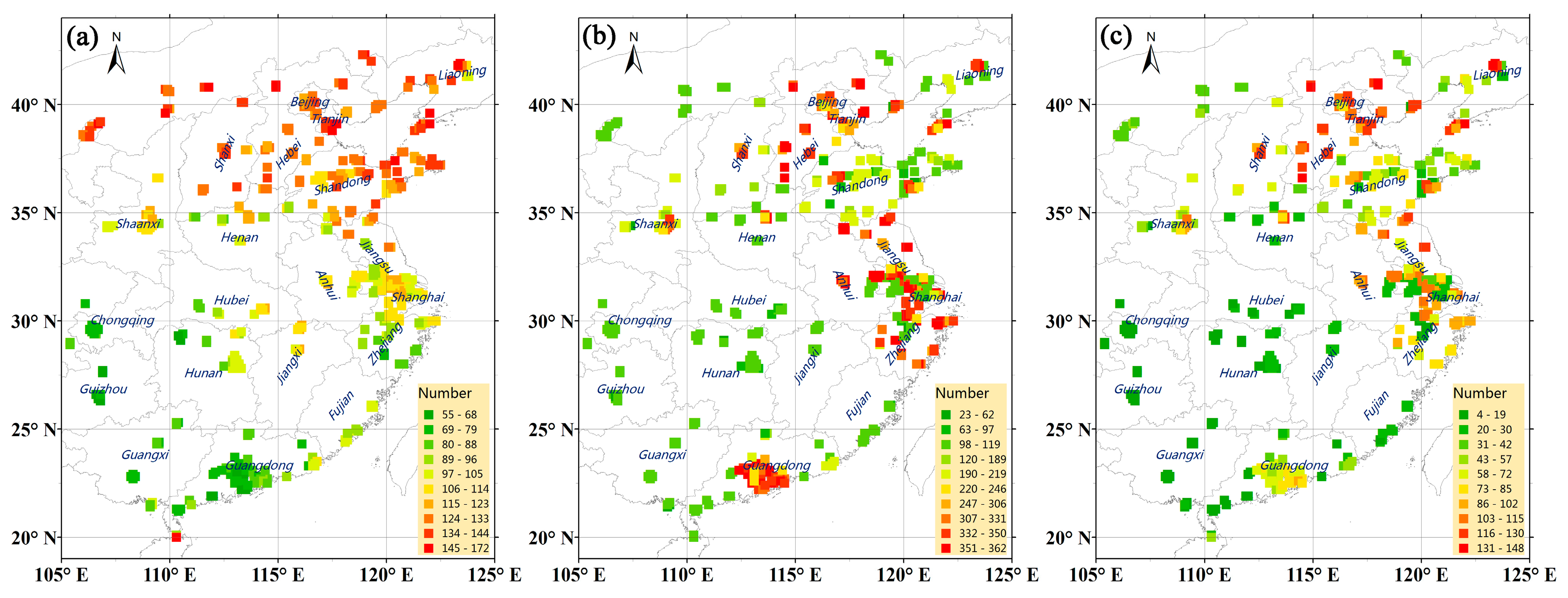
To correlate the ground-based measurements with satellite data, the 715 ambient monitoring stations in the central-eastern China were merged into 509 stations by averaging all of the measurements within a grid of 0.1 × 0.1°. For the 509 grid cells, the total numbers of satellites and ambient monitoring observations are 54,867 (Figure 2a) and 110,545 (Figure 2b), respectively. Combining the satellite and ground observations, there are 31,463 valid data pairs (Figure 2c). The spatial distribution of the numbers of filtered satellite observations in Figure 2a shows a north-south difference, which is likely due to a higher cloud fraction over southern China. These 509 stations with total 31,463 dataset were divided randomly into 10 groups. The model fitting and cross-validation process was repeated 10 times, for every time one group was used for the cross-validation and the rest were used to train the fitting model until all groups were entered into the cross-validation once, thereby creating out-of-sample predictions for all the stations [42]. To be more specific, all of the 31,463 datasets were used both in the fitting and the cross-validation.

Some statistical indicators were employed to quantitatively assess the model performances. They are the coefficient of determination (R²), whose higher value indicating better fitting accuracy, the root mean square error (RSME), that is sensitive to both systematic and random errors, the mean absolute difference (MAD), that measures the mean error magnitude, and the mean absolute percentage error (MAPE), which characterizes the prediction accuracy of a statistical model.

4. Results and Discussion

4.1. Spatio-Temporal Non-Stationarities between Tropospheric-Columnar and Ground Level NO₂

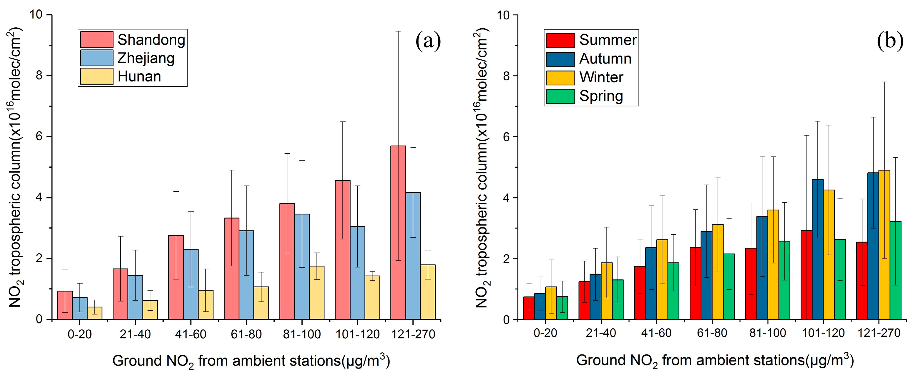
According to previous studies [43,44], the tropospheric NO₂ profiles show a large spatial-temporal variation. It is necessary to assess the impact of the spatio-temporal non-stationarities on the satellite-estimated ground level NO₂ concentrations. Lamsal et al. [38] showed that OMI retrievals are underestimated in urban regions and overestimated in remote areas about 20%. To isolate the influence of different land covers types, 293 pure urban grids and corresponding ambient stations were picked out from the total 509 grids and stations. As shown in Figure 3a, the mean values of tropospheric-columnar and corresponding ground level NO₂ over three provinces in eastern China (see also Figure 1) i.e., Shandong, Zhejiang, and Hunan, are compared. The mean values of OMI tropospheric NO₂ columns of the three provinces are different when the column data is composited with respect to the ground level NO₂ mass concentrations from ambient monitoring stations. This is related to the spatial difference in tropospheric NO₂ profiles due to different topographies and meteorological conditions. Moreover, the mean values of OMI tropospheric NO₂ columns in summer (May to July 2013), autumn (August to October 2013), winter (November 2013 to January 2014), and spring (February to April 2014) are compared in Figure 3b. The relationship between the NO₂ columns and ground level NO₂ shows a significant seasonal variation. The NO₂ columns in winter and autumn are higher than those in summer and spring when the values of ground level NO₂ are at the same level. This seasonal difference is more notable when ground concentrations increase, which is likely because of the longer lifetime of NO₂ in winter and autumn as compared to that in summer and spring. Consequently, it can exist for a longer time in the upper layer in the case of high ground emissions. The numbers of satellite observations used in Figure 3a,b are given in

Table 2. Numbers of satellite observations used in Figure 3a.

Province	Ground Level NO2 Mass Concentrations
	0–20	21–40	41–60	61–80	81–100	101–120	121–270
Shandong	1002	1265	611	299	126	68	79
Zhejiang	1371	1240	491	156	57	37	33
Hunan	66	101	57	24	13	3	2

and

Table 3. Numbers of satellite observations used in Figure 3b.

Season	Ground Level NO2 Mass Concentrations
	0–20	21–40	41–60	61–80	81–100	101–120	121–270
Summer	1567	1137	283	94	23	3	4
Autumn	1815	1423	436	169	51	21	13
Winter	1059	1785	1248	653	313	174	175
Spring	2022	2336	870	296	96	37	30

, respectively. It should be pointed out that the numbers of satellite observations for high ground level NO₂ (>100 μg/m³) are less than five in Hunan and in summer.

4.2. Comparison between Model Fitted and Ground-Observed NO₂

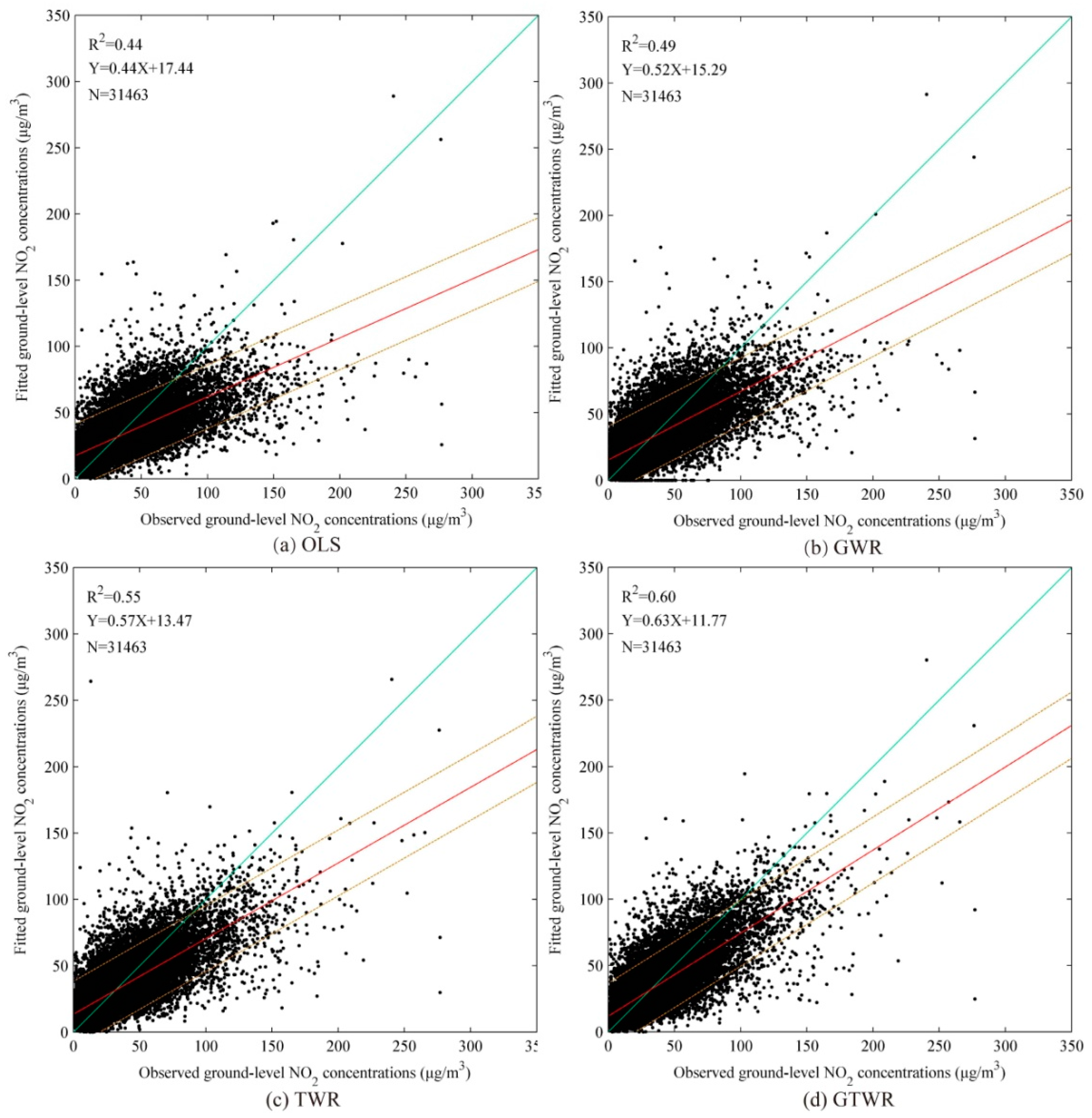
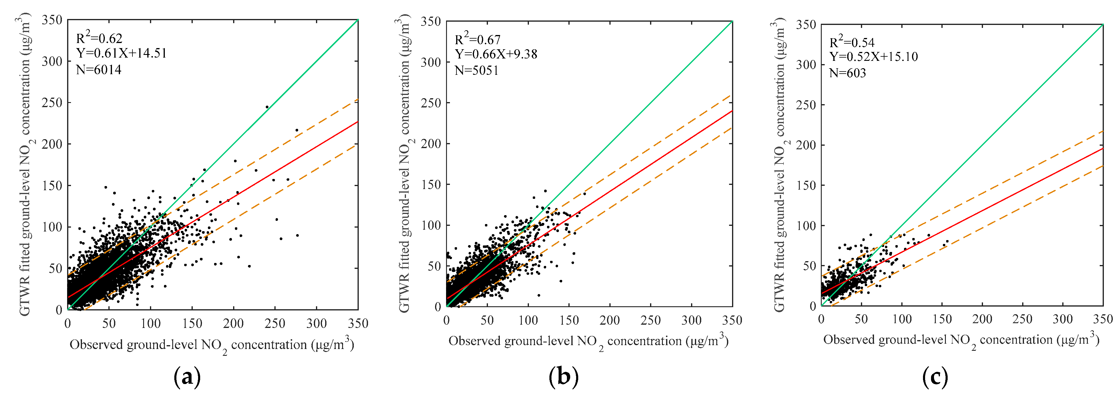
The ordinary least squares (OLS), GWR, temporally weighted regression (TWR), and GTWR models were tested using the same datasets. As shown in

Table 4. Quantitative assessment of model-fitting through ordinary least squares (OLS), geographically weighted regression (GWR), temporally weighted regression (TWR), and GTWR.

Model	R2	RMSE (μg/m3)	MAD (μg/m3)	MAPE (%)
OLS	0.45	0.11	12.54	73.24
GWR	0.55	0.10	11.16	61.10
TWR	0.61	0.09	10.59	60.52
GTWR	0.69	0.08	9.38	52.10

and

Table 5. Quantitative assessment of cross-validation through OLS, GWR, TWR, and GTWR.

Model	R2	RMSE (μg/m3)	MAD (μg/m3)	MAPE (%)
OLS	0.44	0.33	12.57	73.45
GWR	0.49	0.31	12.09	68.83
TWR	0.55	0.29	11.27	64.63
GTWR	0.60	0.28	10.68	60.19

, the OLS performance reveals that the tropospheric NO₂ columns are potentially useful for ground level NO₂ with R² of 0.45 and 0.44 for fitting and validation, respectively. The TWR outperforms the GWR with significant increases of R² values from 0.55 and 0.49 to 0.61 and 0.55. This suggests that the temporal non-stationarity is more dominant than the spatial non-stationarity between the tropospheric NO₂ columns and ground level NO₂. Among the four models, the GTWR has the best performance in both model-fitting and cross-validation with the highest R² and lowest errors (RMSE, MAD, and MAPE). Nevertheless, the GTWR regression shows a slight over-fitting, i.e., the R² generated from the cross-validation is 0.09 smaller than that from the model-fitting. In addition, the scatter plots in Figure 4 shows the largest correlation slope and the smallest intercept for the GTWR model. It is worth noting that all of the regression line slopes for the four models are less than 1. Figure 5 is present to assess the impact of the numbers of valid observations on the GTWR performance. The R² over Hunan (Figure 5a) is smaller than those over Shandong (Figure 5b) and Zhejiang (Figure 5c), due to less observations.

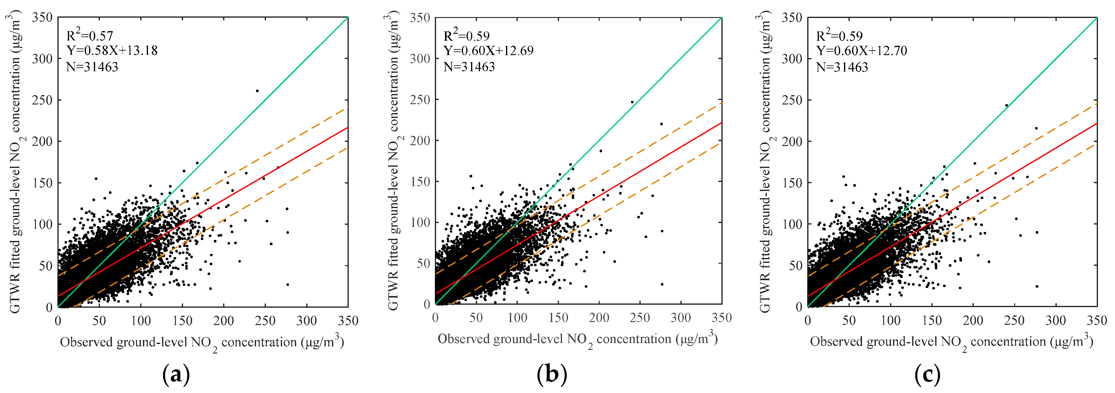
There are three possible errors in the estimation of ground level NO₂ concentrations using the satellite-based GTWR model. First, satellite data are collected over an area of hundreds of km², while in-situ measurements are point observations. Second, the errors in the retrieval of OMI tropospheric NO₂ columns are underestimated in urban regions and overestimated in remote areas by about −20% and 20%, respectively [38]. Third, the uncertainty in the meteorological parameters can affect the vertical distribution of tropospheric NO₂. Zhang et al. [45] validated the NCEP FNL data against meteorological station data over Henan, China during 2012, and they found the errors of air temperature and pressure are −3~2 K and −10~10 hPa, respectively. We introduced the expected random errors (Gaussian distribution) from the tropospheric NO₂ columns, air temperature, and air pressure, to assess their impact on the performance of the GTWR model. As shown in

Table 6. Quantitative assessment of GTWR cross-validation with random errors from tropospheric NO₂ columns, air temperature, and air pressure.

Variations	Random Errors	R2	RMSE (μg/m3)	MAD (μg/m3)	MAPE (%)
Tropospheric NO2 columns	20%	0.57	0.29	11.01	62.40
Air temperature	2 K	0.59	0.28	10.75	61.11
Air pressure	10 hPa	0.59	0.28	10.75	60.86

and Figure 6, our model uncertainties are relatively low with the expected uncertainties from the model parameters.

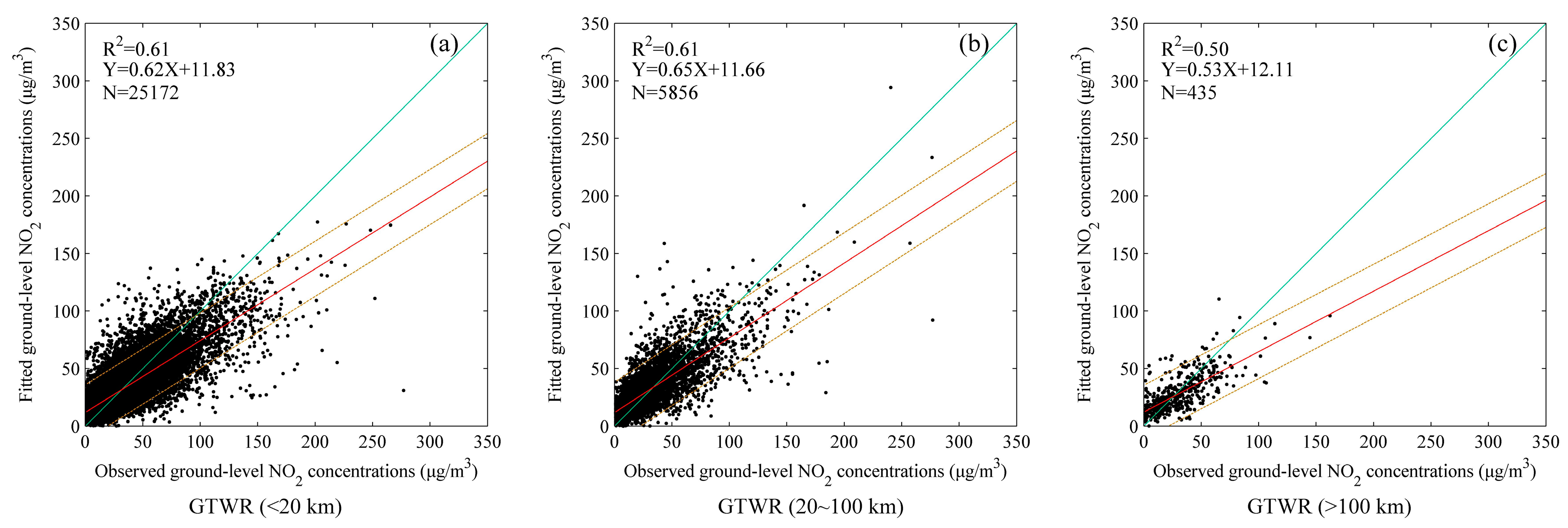
In the GTWR model, the smaller the spatio-temporal distance between two samples is, the greater weight coefficients are given. As illustrated in Figure 7, the GTWR performs much better than the OLS for the samples whose distances to the ambient monitoring stations are within 100 km, whereas the GTWR performance is worse than the OLS (0.41 versus 0.44 for R²) for the samples that are more than 100 km away from the ambient monitoring stations. In the regions like Anhui, Jiangxi, and Fujian, where the ambient monitoring stations are very sparse and unevenly distributed, the nearest samples are mostly more than 100 km away. Hence, we used adjustable bandwidths according to the sample distances rather than the fixed ones. As compared to Figure 7, the R² in Figure 8 improves from 0.41 to 0.50 for the samples with larger distances (>100 km) after adjusting the bandwidth.

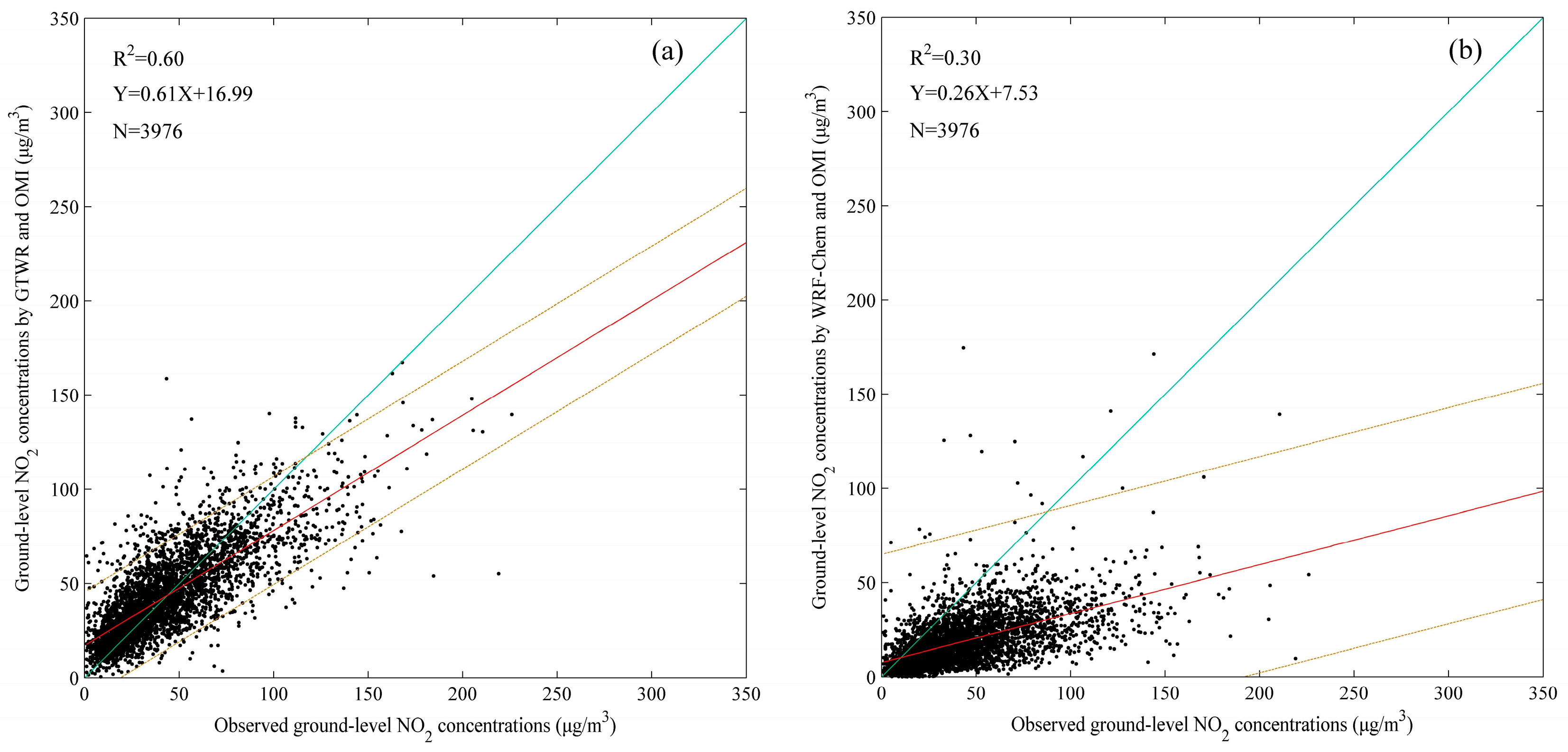
To compare the GTWR method with the chemistry transport model (CTM) approach, we generated the tropospheric NO₂ profiles by using a WRF-Chem model with the monthly MIX Asian anthropogenic emission inventory [46]. This emission inventory has a spatial resolution of 0.25 × 0.25° and involves four emission categories, including industry, power, transport, and residential. The model has 20 vertical levels and the top level pressure is 200 hPa. The RADM2 chemical mechanism is used for the gas-phase chemical reaction calculations. The Modal Aerosol Dynamics Model for Europe-MADE/SORGAM is chosen for the aerosol scheme. Then, we estimated the ground level NO₂ concentrations in January 2014 over central-eastern China using the approach described by Lamsal et al. [18,19]. As shown in Figure 9, the result of the GTWR fitted is much better than the WRF-Chem. Recently, Gu et al. [43] estimated the ground level NO₂ over China using the chemistry transport model approach with the Community Multi-scale Air Quality (CMAQ) model by considering the influence of China’s high atmospheric pollution on obtaining the vertical distribution of tropospheric NO₂ profiles. They achieved a correlation coefficient (R) of 0.80 for January 2014, which is comparable to the coefficient of determination (R²) of 0.60 obtained by the GTWR.

To further evaluate the performance of the GTWR model, the comparison of the annual mean of NO₂ concentrations between the model-fitted and ground-observed data is given in Figure 10. Overall, the NO₂ concentrations estimated by the GTWR model agree well with the ground-based measurements. More than 90% of the cross-validation stations possess low mean discrepancies of less than 10 μg/m³.

4.3. Spatial Distribution of GTWR Fitted Ground-Observed NO₂

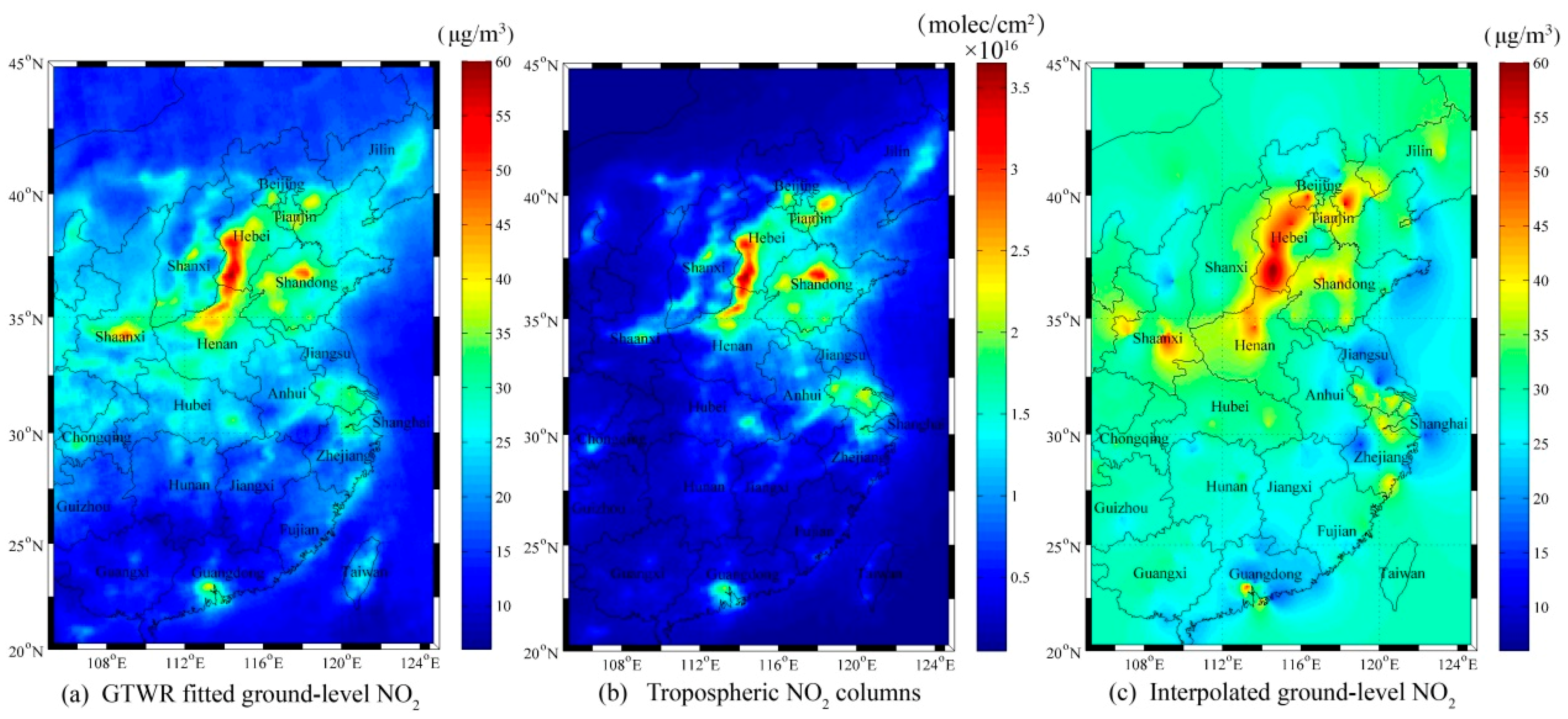
The spatial distributions of annual mean NO₂ values are shown in Figure 11. The fitted ground-observed NO₂ concentrations by GTWR in (a) have similar spatial patterns to the satellite tropospheric NO₂ columns in (b). The concentrations are comparable to the interpolated in situ observations using the Kriging method in (c) over the region with high values. Importantly, in the areas without monitoring stations (e.g., southern Jiangxi and northern Fujian), Figure 11a provides more reasonable estimations that are overestimated in Figure 11c. In Figure 11a, high NO₂ concentrations are clustered in the regions of North China Plain, Yangtze River Delta, and Pearl River Delta. Especially, the NO₂ concentrations in southern Hebei, northern Henan, central Shandong, and southern Shaanxi exceeded the Level 2 standard of the Chinese National Ambient Air Quality Standard (40 μg/m³). Figure 12 denotes dramatic seasonal changes in the spatial distribution of GTWR fitted ground level NO₂. Unparalleled high values are found in winter, while the lowest values are found in summer.

4.4. Population-Weighted Ground Level NO₂ Concentrations

Given the NO₂ toxicity to human health, it is necessary to evaluate population exposure levels over different provinces. Traditionally, the province-level mean NO₂ concentration provided by the Chinese environmental protection agencies are the arithmetic means of all values in administered cities. Here, we calculated the annual mean population-weighted NO₂ (AMPNO₂) concentrations by using Equation (20). The annual mean NO₂ concentrations (AMNO₂) and AMPNO₂ of 17 provinces in central-eastern China are summarized in

Table 7. Annual mean NO₂ (AMNO₂) concentrations and population-weighted NO₂ (AMPNO₂) concentrations for 17 provinces in central-eastern China.

Province	AMNO2 (μg/m3)	AMPNO2 (μg/m3)	Population (Millions)	Proportion of People Exposed to High-Level NO2 Concentrations (>30 μg/m3)
Hebei	27.47	35.23	108.74	74.14%
Tianjin	31.67	34.38	23.04	85.84%
Beijing	26.09	33.86	33.73	87.03%
Shaanxi	25.66	32.43	53.35	55.78%
Henan	29.73	32.12	132.31	56.30%
Shandong	30.21	31.3	139.65	58.28%
Shanxi	24.59	28.43	54.76	46.07%
Shanghai	26.02	27.87	33.56	14.61%
Jiangsu	24.86	27.04	113.16	35.40%
Hubei	23.4	25.56	81.48	19.49%
Chongqing	22.13	25.29	38.34	21.16%
Zhejiang	21.17	25.08	76.21	21.03%
Anhui	21.8	23.48	84.41	0%
Guangdong	14.91	21.09	138.15	18.92%
Fujian	16.9	18.76	47.94	0%
Jiangxi	15.76	17.23	62.96	0%
Hunan	15.55	16.9	89.44	0%

. AMPNO2 is higher than AMNO2 for all of the provinces, especially for densely populated provinces, e.g., Hebei, Beijing, and Guangdong. People from these 17 provinces except Anhui, Fujian, Jiangxi, and Hunan, are exposed to high-level NO₂ concentrations (>30 μg/m³). Heibei, Tianjin, and Beijing suffer from the most serious NO₂ pollution, with more than 70% of people affected by high-level NO₂. The satellite-estimated ground level NO₂ concentration is observed at afternoon (13:00–15:00) leading to underestimated annual mean values.

5. Conclusions

In this study, a satellite-based GTWR model has been applied to estimate ground level NO₂ concentrations over central-eastern China. OMI tropospheric NO₂ columns, together with ambient monitoring station measurements and meteorological data from May 2013 to April 2014 were considered. The results show that the GTWR model produces the highest cross-validation R² (0.60) and the lowest errors (RMSE, MAD, and MAPE), in comparison with other models, i.e., OLS, GWR, and TWR. The model performance is significantly correlated with the meteorological parameters that likely describe the NO₂ vertical profile shapes. Our method is better than or comparable to the CTM method.

The satellite-estimated spatial distribution of annual mean NO₂ shows a similar spatial pattern to the tropospheric NO₂ column and possesses similar value with the in situ observation. High annual mean NO₂ concentrations (>40 μg/m³) are found in southern Hebei, northern Henan, central Shandong, and southern Shaanxi. Seasonal changes in the spatial distribution of ground level NO₂ are easily identifiable with unparalleled high values in winter and the lowest values in summer. The population-weighted NO₂ demonstrates that people who lived in densely populated areas are more likely to be exposed to high NO₂ pollution.

One of the major error sources in the estimation of ground level NO₂ concentrations using OMI data is the spatial gradient and the horizontal inhomogeneity between individual satellite pixels. In September 2017, the TROPOMI/S5P will be launched and measure tropospheric NO₂ columns with a higher spatial resolution (7 km × 7 km) [47], which enables an improved accuracy in the ground level NO₂ estimation.

References

1. Gauderman, W.J.; Gilliland, G.F.; Vora, H.; Avol, E.; Stram, D.; Mcconnell, R.; Thomas, D.; Lurmann, F.; Margolis, H.G.; Rappaport, E.B. Association between air pollution and lung function growth in southern California children. Am. J. Respir. Crit. Care Med. 2000, 162, 1383–1390. [Google Scholar] [CrossRef] [PubMed]
2. Chiusolo, M.; Cadum, E.; Stafoggia, M.; Galassi, C.; Berti, G.; Faustini, A.; Bisanti, L.; Vigotti, M.A.; Patrizia, D.M.; Cernigliaro, A. Short-term effects of nitrogen dioxide on mortality and susceptibility factors in 10 Italian cities: The EpiAir study. Environ. Health Perspect. 2011, 119, 1233. [Google Scholar] [CrossRef] [PubMed]
3. Stieb, D.M.; Burnett, R.T.; Smithdoiron, M.; Brion, O.; Shin, H.H.; Economou, V. A new multipollutant, no-threshold air quality health index based on short-term associations observed in daily time-series analyses. J. Air Waste Manag. Assoc. 2008, 58, 435–450. [Google Scholar] [PubMed]
4. Sioris, C.E.; Kurosu, T.P.; Martin, R.V.; Chance, K. Stratospheric and tropospheric NO2 observed by SCIAMACHY: First results. Adv. Space Res. 2004, 34, 780–785. [Google Scholar] [CrossRef]
5. Boersma, K.F.; Eskes, H.J.; Veefkind, J.P.; Brinksma, E.J.; van der A, R.J.; Sneep, M.; Oord, G.H.J.V.; Levelt, P.F.; Stammes, P.; Gleason, J.F. Near-real time retrieval of tropospheric NO2 from OMI. Atmos. Chem. Phys. Discuss. 2006, 6, 12301–12345. [Google Scholar] [CrossRef]
6. Valks, P.; Pinardi, G.; Richter, A.; Lambert, J.C. Operational total and tropospheric NO2 column retrieval for GOME-2. Atmos. Meas. Tech. 2011, 4, 1491. [Google Scholar] [CrossRef]
7. Irie, H.; Boersma, F.; Kanaya, Y.; Takashima, H.; Xiaole, P.; Wang, Z. Quantitative bias estimates for tropospheric NO2 columns retrieved from SCIAMACHY, OMI, and GOME-2 using a common standard for East Asia. Atmos. Meas. Tech. 2012, 5, 2403–2411. [Google Scholar] [CrossRef]
8. Hassinen, S.; Balis, D.; Bauer, H.; Begoin, M.; Delcloo, A.; Eleftheratos, K.; Gimeno Garcia, S.; Granville, J.; Grossi, M.; Hao, N. Overview of the O3M SAF GOME-2 operational atmospheric composition and UV radiation data products and data availability. Atmos. Meas. Tech. 2016, 9, 383–407. [Google Scholar] [CrossRef] [Green Version]
9. Richter, A.; Burrows, J.P.; Nüss, H.; Granier, C.; Niemeier, U. Increase in tropospheric nitrogen dioxide over China observed from space. Nature 2005, 437, 129–132. [Google Scholar] [CrossRef] [PubMed]
10. Van Der, A.R.J.; Peters, D.; Eskes, H.; Boersma, K.F.; Roozendael, M.V.; Smedt, I.D.; Kelder, H.M. Detection of the trend and seasonal variation in tropospheric NO2 over China. J. Geophys. Res. Atmos. 2006, 111. [Google Scholar] [CrossRef]
11. Zhang, Q.; Geng, G.N.; Wang, S.W.; Richter, A.; He, K.B. Satellite remote sensing of changes in NOx emissions over China: 1996–2010. Chin. Sci. Bull. 2012, 57. [Google Scholar] [CrossRef]
12. Zhang, L.; Lee, C.S.; Zhang, R.; Chen, L. Spatial and temporal evaluation of long term trend (2005–2014) of OMI retrieved NO2 and SO2 concentrations in Henan Province, China. Atmos. Environ. 2017, 154, 151–166. [Google Scholar] [CrossRef]
13. Liu, F.; Beirle, S.; Zhang, Q.; Dörner, S.; He, K.; Wagner, T. NOx lifetimes and emissions of cities and power plants in polluted background estimated by satellite observations. Atmos. Chem. Phys. 2016, 16, 5283–5298. [Google Scholar] [CrossRef]
14. Petritoli, A.; Bonasoni, P.; Giovanelli, G.; Ravegnani, F.; Kostadinov, I.; Bortoli, D.; Weiss, A.; Schaub, D.; Richter, A.; Fortezza, F. First comparison between ground-based and satellite-borne measurements of tropospheric nitrogen dioxide in the Po basin. J. Geophys. Res. Atmos. 2004, 109. [Google Scholar] [CrossRef]
15. Vienneau, D.; Hoogh, K.D.; Bechle, M.J.; Beelen, R.; Donkelaar, A.V.; Martin, R.V.; Millet, D.B.; Hoek, G.; Marshall, J.D. Western European land use regression incorporating satellite-and ground-based measurements of NO2 and PM10. Environ. Sci. Technol. 2013, 47, 13555–13564. [Google Scholar] [CrossRef] [PubMed]
16. Lee, H.J.; Koutrakis, P. Daily ambient NO2 concentration predictions using satellite ozone monitoring instrument NO2 data and land use regression. Environ. Sci. Technol. 2014, 48, 2305–2311. [Google Scholar] [PubMed]
17. Hoek, G.; Eeftens, M.; Beelen, R.; Fischer, P.; Brunekreef, B.; Boersma, K.F.; Veefkind, P. Satellite NO2 data improve national land use regression models for ambient NO2 in a small densely populated country. Atmos. Environ. 2015, 105, 173–180. [Google Scholar] [CrossRef]
18. Lamsal, L.N.; Martin, R.V.; Donkelaar, A.V.; Steinbacher, M.; Celarier, E.A.; Bucsela, E.; Dunlea, E.J.; Pinto, J.P. Ground level nitrogen dioxide concentrations inferred from the satellite-borne Ozone Monitoring Instrument. J. Geophys. Res. Atmos. 2008, 113, 280–288. [Google Scholar] [CrossRef]
19. Lamsal, L.N.; Duncan, B.N.; Yoshida, Y.; Krotkov, N.A.; Pickering, K.E.; Streets, D.G.; Lu, Z. US NO2 trends (2005–2013): EPA Air Quality System (AQS) data versus improved observations from the Ozone Monitoring Instrument (OMI). Atmos. Environ. 2015, 110, 0e143. [Google Scholar] [CrossRef]
20. Kharol, S.K.; Martin, R.V.; Philip, S.; Boys, B.; Lamsal, L.N.; Jerrett, M.; Brauer, M.; Crouse, D.L.; Mclinden, C.; Burnett, R.T. Assessment of the magnitude and recent trends in satellite-derived ground-level nitrogen dioxide over North America. Atmos. Environ. 2015, 118, 236–245. [Google Scholar] [CrossRef]
21. Chan, K.L.; Hartl, A.; Lam, Y.F.; Xie, P.H.; Liu, W.Q.; Cheung, H.M.; Lampel, J.; Pöhler, D.; Li, A.; Xu, J. Observations of tropospheric NO2 using ground based MAX-DOAS and OMI measurements during the Shanghai World Expo 2010. Atmos. Environ. 2015, 119, 45–58. [Google Scholar] [CrossRef]
22. Kim, D.; Lee, H.; Hong, H.; Choi, W.; Yun, G.L.; Park, J. Estimation of surface NO2 volume mixing ratio in four metropolitan cities in Korea using multiple regression models with OMI and AIRS Data. Remote Sens. 2017, 9, 627. [Google Scholar] [CrossRef]
23. Song, W.; Jia, H.; Huang, J.; Zhang, Y. A satellite-based geographically weighted regression model for regional PM2.5 estimation over the Pearl River Delta region in China. Remote Sens. Environ. 2014, 154, 1–7. [Google Scholar] [CrossRef]
24. You, W.; Zang, Z.; Zhang, L.; Li, Z.; Chen, D.; Zhang, G. Estimating ground-level PM10 concentration in northwestern China using geographically weighted regression based on satellite AOD combined with CALIPSO and MODIS fire count. Remote Sens. Environ. 2015, 168, 276–285. [Google Scholar] [CrossRef]
25. Zou, B.; Pu, Q.; Bilal, M.; Weng, Q.; Zhai, L.; Nichol, J.E. High-resolution satellite mapping of fine particulates based on geographically weighted regression. IEEE Geosci. Remote Sens. Lett. 2016, 13, 495–499. [Google Scholar] [CrossRef]
26. You, W.; Zang, Z.; Zhang, L.; Li, Y.; Pan, X.; Wang, W. National-scale estimates of ground-level PM2.5 concentration in China using geographically weighted regression based on 3 km resolution MODIS AOD. Remote Sens. 2016, 8, 184. [Google Scholar] [CrossRef]
27. Bai, Y.; Wu, L.; Qin, K.; Zhang, Y.; Shen, Y.; Zhou, Y. A geographically and temporally weighted regression model for ground-level PM2.5 estimation from satellite-derived 500 m resolution AOD. Remote Sens. 2016, 8, 262. [Google Scholar] [CrossRef]
28. Guo, Y.; Tang, Q.; Gong, D.Y.; Zhang, Z. Estimating ground-level PM2.5 concentrations in Beijing using a satellite-based geographically and temporally weighted regression model. Remote Sens. Environ. 2017, 198, 140–149. [Google Scholar] [CrossRef]
29. Levelt, P.F.; Oord, G.H.J.V.; Dobber, M.R.; Malkki, A.; Visser, H.; Vries, J.D.; Stammes, P.; Lundell, J.O.V.; Saari, H. The ozone monitoring instrument. IEEE Trans. Geosci. Remote Sens. 2006, 44, 1093–1101. [Google Scholar] [CrossRef]
30. Platt, U.; Stutz, J. Differential Absorption Spectroscopy. In Differential Optical Absorption Spectroscopy; Springer: Berlin/Heidelberg, Germany, 2008; pp. 135–174. [Google Scholar]
31. Bucsela, E.J.; Krotkov, N.A.; Celarier, E.A.; Lamsal, L.N. A new stratospheric and tropospheric NO2 retrieval algorithm for nadir-viewing satellite instruments: Applications to OMI. Atmos. Meas. Tech. 2013, 6, 2607. [Google Scholar] [CrossRef]
32. Douglass, A.R.; Stolarski, R.S.; Strahan, S.E.; Connell, P.S. Radicals and reservoirs in the GMI chemistry and transport model: Comparison to measurements. J. Geophys. Res. Atmos. 2004, 109. [Google Scholar] [CrossRef]
33. Bucsela, E.J.; Celarier, E.A.; Gleason, J.L.; Krotkov, N.A.; Lamsal, L.N.; Marchenko, S.V.; Swartz, W.H. OMNO2 Readme Document Data Product Version 3.0. 2016. Available online: https://aura.gesdisc.eosdis.nasa.gov/data//Aura_OMI_Level2/OMNO2.003/doc/README.OMNO2.pdf (accessed on 16 September 2016).
34. Boersma, K.F.; Eskes, H.J.; Brinksma, E.J. Error analysis for tropospheric NO2 retrieval from space. J. Geophys. Res. Atmos. 2004, 109. [Google Scholar] [CrossRef]
35. Boersma, F.; Dirksen, R.; Brunner, D.; Zhou, Y.; Huijnen, V.; Eskes, H.; Veefkind, P.; Kleipool, Q.; Dobber, M.; Stammes, P. An improved retrieval of tropospheric NO2 columns from the Ozone Monitoring Instrument. Atmos. Meas. Tech. 2011, 4, 1905–1928. [Google Scholar] [CrossRef]
36. Hong, H.; Lee, H.; Kim, J.; Jeong, U.; Ryu, J.; Lee, D.S. Investigation of simultaneous effects of aerosol properties and aerosol peak height on the air mass factors for space-borne NO2 retrievals. Remote Sens. 2017, 9, 208. [Google Scholar] [CrossRef]
37. Wang, Y.; Beirle, S.; Lampel, J.; Koukouli, M.; De Smedt, I.; Theys, N.; Li, A.; Wu, D.; Xie, P.; Liu, C. Validation of OMI, GOME-2A and GOME-2B tropospheric NO2, SO2 and HCHO products using MAX-DOAS observations from 2011 to 2014 in Wuxi, China: Investigation of the effects of priori profiles and aerosols on the satellite products. Atmos. Chem. Phys. 2017, 17, 5007. [Google Scholar] [CrossRef]
38. Lamsal, L.N.; Krotkov, N.A.; Celarier, E.A.; Swartz, W.H.; Pickering, K.E.; Bucsela, E.J.; Martin, R.V.; Philip, S.; Irie, H.; Cede, A. Evaluation of OMI operational standard NO2 column retrievals using in situ and surface-based NO2 observations. Atmos. Chem. Phys. 2014, 14, 11587–11609. [Google Scholar] [CrossRef]
39. Wang, S.; Zhang, Q.; Martin, R.V.; Philip, S.; Liu, F.; Li, M.; Jiang, X.; He, K. Satellite measurements oversee China’s sulfur dioxide emission reductions from coal-fired power plants. Environ. Res. Lett. 2015, 10, 114015. [Google Scholar] [CrossRef]
40. Huang, B.; Wu, B.; Barry, M. Geographically and temporally weighted regression for modeling spatio-temporal variation in house prices. Int. J. Geogr. Inf. Sci. 2010, 24, 383–401. [Google Scholar] [CrossRef]
41. Beelen, R.; Hoek, G.; Pebesma, E.; Vienneau, D.; Hoogh, K.D.; Briggs, D.J. Mapping of background air pollution at a fine spatial scale across the European union. Sci. Total Environ. 2009, 407, 1852–1867. [Google Scholar] [CrossRef] [PubMed]
42. Young, M.T.; Bechle, M.J.; Sampson, P.D.; Szpiro, A.A.; Marshall, J.D.; Sheppard, L.; Kaufman, J.D. Satellite-based NO2 and model validation in a national prediction model based on universal Kriging and land-use regression. Environ. Sci. Technol. 2016, 50, 3686–3694. [Google Scholar] [CrossRef] [PubMed]
43. Gu, J.; Chen, L.; Yu, C.; Li, S.; Tao, J.; Fan, M.; Xiong, X.; Wang, Z.; Shang, H.; Su, L. Ground-level NO2 concentrations over China inferred from the Satellite OMI and CMAQ Model simulations. Remote Sens. 2017, 9, 519. [Google Scholar] [CrossRef]
44. Ma, J.Z.; Beirle, S.; Jin, J.L.; Shaiganfar, R.; Yan, P.; Wagner, T. Tropospheric NO2 vertical column densities over Beijing: Results of the first three years of ground-based MAX-DOAS measurements (2008–2011) and satellite validation. Atmos. Chem. Phys. 2013, 13, 1547–1567. [Google Scholar] [CrossRef]
45. Zhang, Y.T.; Chen, Y.D. Error comparison analysis between FNL data and observation data of air temperature, air pressure and ground temperature in Henan Province in 2012. Meteorol. Environ. Sci. 2014, 37, 93–97. (In Chinese) [Google Scholar]
46. Li, M.; Zhang, Q.; Kurokawa, J.; Woo, J.H.; He, K.; Lu, Z.; Ohara, T.; Song, Y.; Streets, D.G.; Carmichael, G.R. MIX: A mosaic Asian anthropogenic emission inventory under the international collaboration framework of the MICS-Asia and HTAP. Atmos. Chem. Phys. 2017, 17, 935. [Google Scholar] [CrossRef]
47. Veefkind, J.P.; Aben, I.; Mcmullan, K.; Förster, H.; Vries, J.D.; Otter, G.; Claas, J.; Eskes, H.J.; Haan, J.F.D.; Kleipool, Q. TROPOMI on the ESA Sentinel-5 Precursor: A GMES mission for global observations of the atmospheric composition for climate, air quality and ozone layer applications. Remote Sens. Environ. 2012, 120, 70–83. [Google Scholar] [CrossRef]
Figure 1. Study area and locations of ambient monitoring stations.
Remotesensing 09 00950 g001
Figure 2. Numbers of satellite observations (a), ambient monitoring observations (b), and valid satellite and ground observation pairs (c) for 593 grid cells.
Remotesensing 09 00950 g002
Figure 3. Mean values of tropospheric NO2 columns (×1016 molec/cm2) in different provinces (a) and different seasons (b) when the column data is composited with respect to the ground level NO2 mass concentrations observed at 293 pure urban ambient monitoring stations. Error bars stand for one standard deviation.
Remotesensing 09 00950 g003
Figure 4. Scatter plots between the observed NO2 and predicted NO2 concentrations using OLS (a), GWR (b), TWR (c), and GTWR (d) for cross validation over central-eastern China from May 2013 to April 2014.
Remotesensing 09 00950 g004
Figure 5. Scatter plots between the observed NO2 and predicted NO2 concentrations for cross validation over Shandong (a), Zhejiang (b), and Hunan (c) from May 2013 to April 2014.
Remotesensing 09 00950 g005
Figure 6. Scatter plots between the observed NO2 and GTWR predicted NO2 concentrations with random errors from tropospheric NO2 columns (20%) (a), air temperature (2 K) (b), and air pressure (10 hPa) (c) over central-eastern China from May 2013 to April 2014.
Remotesensing 09 00950 g006
Figure 7. Scatter plots between the observed NO2 and predicted NO2 concentrations using GTWR ((ac) and OLS (df) for samples with different distances (a,d) <20 km; (b,e) 20–100 km; (c,f) >100 km) for cross validation over central-eastern China from May 2013 to April 2014.
Remotesensing 09 00950 g007
Figure 8. Scatter plots between the observed NO2 and GTWR predicted NO2 concentrations for samples with different distances ((a) <20 km; (b) 20-100 km; (c) >100 km) after adjusting the bandwidth for cross validation over central-eastern China from May 2013 to April 2014.
Remotesensing 09 00950 g008
Figure 9. Scatter plots between the observed NO2 and predicted NO2 concentrations by GTWR (a) and WRF-Chem (b) for cross validation over central-eastern China in January 2014.
Remotesensing 09 00950 g009
Figure 10. Annual means of observed NO2 and fitted NO2 by the GTWR model for all 509 stations.
Remotesensing 09 00950 g010
Figure 11. Spatial distribution of annual mean values of (a) ground level NO2 concentrations fitted by GTWR model, (b) NO2 tropospheric columns, and (c) ground level NO2 concentrations interpolated by Kriging method.
Remotesensing 09 00950 g011
Figure 12. Spatial distribution of seasonal mean values of GTWR fitted (upper) and Kriging interpolated (lower) ground level NO2 concentrations.
Remotesensing 09 00950 g012