Multi-Objective Optimizations of a Serpentine Micromixer with Crossing Channels at Low and High Reynolds Numbers


Department of Mechanical Engineering, Inha University, Incheon 22212, Korea
*
Author to whom correspondence should be addressed.
Micromachines 2018, 9(3), 110; https://doi.org/10.3390/mi9030110
Submission received: 24 January 2018
/
Revised: 26 February 2018
/
Accepted: 1 March 2018
/
Published: 4 March 2018
(This article belongs to the Special Issue Passive Micromixers)
Abstract
:In order to maximize the mixing performance of a micromixer with an integrated three-dimensional serpentine and split-and-recombination configuration, multi-objective optimizations were performed at two different Reynolds numbers, 1 and 120, based on numerical simulation. Numerical analyses of fluid flow and mixing in the micromixer were performed using three-dimensional Navier-Stokes equations and convection-diffusion equation. Three dimensionless design variables that were related to the geometry of the micromixer were selected as design variables for optimization. Mixing index at the exit and pressure drop through the micromixer were employed as two objective functions. A parametric study was carried out to explore the effects of the design variables on the objective functions. Latin hypercube sampling method as a design-of-experiment technique has been used to select design points in the design space. Surrogate modeling of the objective functions was performed by using radial basis neural network. Concave Pareto-optimal curves comprising of Pareto-optimal solutions that represents the trade-off between the objective functions were obtained using a multi-objective genetic algorithm at Re = 1 and 120. Through the optimizations, maximum enhancements of 18.8% and 6.0% in mixing index were achieved at Re = 1 and 120, respectively.
1. Introduction
Microfluidics is related to an expeditiously emerging technology enabling manipulation and control of minute volumes of fluids with high accuracy in a miniaturized system for various fluidic functions, such as transporting, metering, valving, mixing, reacting, and separating [1,2]. Micromixer is an integral component of the microfluidic systems that have promising impact in the fields of biomedical diagnostics, drug development, and chemical industry [3,4]. Efficient mixing of liquid samples is a challenging task for successful operation of different processes in the microfluidic systems. The flow nature in the microfluidic systems is laminar, due to low Reynolds number. Thus, the mixing of fluid species depends mainly on mass diffusion in the absence of turbulence. However, the diffusion-dependent mixing is relatively slow and ineffective. In order to enhance the mixing performance, numerous methods have been proposed during the last two decades [3,5,6,7].
Depending upon the working principle, micromixers are categorized either as a passive or as an active type. Active micromixers employ external energy sources, such as electrokinetic, ultrasonic vibration and magnetic field to generate flow perturbations inside the microchannel. Although active micromixers generally show excellent mixing capability and control during the mixing, high fabrication cost, and difficulty in integration with microfluidic systems make them less practical. In contrast, passive micromixers that enhance mixing by modifying the microchannel geometry, are being widely developed due to the advantages of simple fabrication and easy integration with the microfluidic systems [3,5,6,7,8].
Over the last two decades, many researchers have proposed different microchannel designs to enhance the mixing performance of passive micromixers. In general, passive micromixers, depending upon the mechanism of mixing, are classified as lamination-based [9,10,11,12,13] or chaotic advection-based [14,15,16,17]. Kim et al. [9] proposed a serpentine laminating micromixer that combines the mixing mechanisms of split-and-recombination (SAR) using successive arrangement of F-shaped mixing units in two layers and chaotic advection through a three-dimensional (3D) serpentine microchannel path. Tofteberg et al. [10] developed a lamination micromixer incorporating a sequence of SAR process with patterning of the channel bottom with grooves. Nimafar et al. [12] proposed an H-micromixer based on SAR process, and compared its mixing performance with those of T- and O-micromixer in a Reynolds number range of 0.08–4.16. The results showed that the H-micromixer achieved 98% mixing at Re = 0.083 due to SAR process, which was much higher than those of the other two micromixers.
Liu et al. [14] proposed a 3D serpentine micromixer with C-shaped repeating units, and experimentally demonstrated its high mixing performance for Reynolds numbers larger than 25. Stroock et al. [15] proposed a micromixer with patterned grooves on the channel bottom to induce chaotic mixing at low Reynolds numbers. Xia et al. [16] proposed two chaotic micromixers consisting of double-layer crossing channels. Their numerical and experimental results demonstrated that chaotic advection that is generated through continuous stretching and folding along with splitting and recombination, even at low Reynolds numbers (Re < 0.2), resulted in high mixing performance. The et al. [18] proposed a shifted trapezoidal blade micromixer that combined several mixing principles, i.e., vortices, transversal flows, and chaotic advection, to attain a stable mixing efficiency of larger than 80% in a wide Reynolds number range of 0.5–100.
Numerical optimization techniques coupled with computational fluid dynamics (CFD) analysis based on 3D Navier-Stokes equations have been widely used as an efficient tool for design of micromixers [19,20,21,22,23]. Ansari and Kim [19,20] optimized geometric parameters of a staggered herringbone groove micromixer (SHM) with grooves at the bottom wall by using radial basis neural network (RBNN) and response surface approximation (RSA) as surrogate models. These optimizations were carried out using mixing index as a single objective function with two or three design variables. Kim et al. [21] performed an optimization of microscale vortex generators in a micromixer using an advanced RSA by considering four geometric design variables. It was found that a mixing uniformity of larger than 95% was obtained within a channel length of 1344 µm with an optimized microchannel configuration. Cortes-Quiroz et al. [22] applied a multi-objective genetic algorithm (MOGA) for shape optimization of a SHM at Re = 1 and 10, by integrating CFD calculations with a surrogate model. In this optimization, a Pareto-optimal front of trade-offs between two objective functions, i.e., mixing index at the exit and pressure drop, was generated by MOGA. Afzal and Kim [23] performed a multi-objective optimization of a SHM with three objective functions, i.e., mixing index at the exit, friction factor, and mixing sensitivity. Hossain and Kim [24] optimized a micromixer with two-layer serpentine crossing channels at Reynolds numbers of 0.2 and 40 by using CFD, surrogate model and MOGA. Kriging metamodel was used as a surrogate model, while mixing index at the exit and pressure drop were used as two objective functions to generate Pareto-optimal front.
In a recent study, Raza et al. [25] proposed a 3D serpentine SAR micromixer with OX-shaped mixing units, and analyzed the flow structure and mixing performance numerically in a wide Reynolds number range of 0.1–200. The proposed micromixer with five mixing units showed excellent mixing performance over the entire range of Reynolds number, through stretching and folding of fluid interface at the crossing channel intersection nodes at low Reynolds numbers and chaotic motion due to the 3D serpentine path at high Reynolds numbers. Especially, the enhancement of mixing performance in low-Re range is noticeable as compared to previous micromixers.
In the present work, multi-objective optimizations have been performed to further enhance the performance of the micromixer proposed by Raza et al. [25], at both low and high Reynolds numbers. Mixing index at the exit of the micromixer and pressure drop though the micromixer were employed as two objective functions. The Pareto-optimal fronts compromising these two objectives were generated using RBNN surrogate model and MOGA. The optimizations were carried out with the two objective functions at the two different Reynolds numbers, Re = 1 and 120. The corresponding Peclet numbers are 1 × 10⁴ and 120 × 104, respectively.
2. Micromixer Geometry
The micromixer configuration, as proposed by Raza et al. [25], has been used for the optimization. The micromixer consists of two repeated OX-shaped mixing units of 3D serpentine SAR structure as shown in Figure 1. The number of mixing units was reduced from five of previous work [25] to two in this work. Chaotic advection through stretching and folding of fluid interface at the X-junction, where the fluids in both the crossing channels are exchanged, enhances mixing at low Reynolds numbers. On the other hand, 3D serpentine path that was created by O-structure promotes mixing by producing chaotic advection at high Reynolds numbers, as explained in the previous study [25].
Values of the geometric parameters for the reference micromixer are listed in Table 1. The traditional method of stacking the polydimethylsiloxane (PDMS) layers can be used to fabricate the proposed micromixer. As described in the previous works [17,26], the micro-molding technology, i.e., soft lithography technique using SU-8 master molds, can be employed to fabricate these PDMS layers.
3. Numerical Analysis
The analyses of fluid flow and mixing inside the micromixer were performed numerically using a commercial CFD code, ANSYS CFX 15.0 (ANSYS, Inc., Canonsburg, PA, USA) [27], based on finite volume approximations. The numerical analysis of steady, incompressible, 3D laminar flow was carried out by solving the continuity and Navier-Stokes equations:
where the symbols ν, ρ, and denote the fluid kinematic viscosity, density, and velocity, respectively. A solution of dye in water and water at a temperature of 20 °C were considered as two working fluids. To model the mass transport of the fluids having constant viscosity and density in the mixing process, a scalar transport equation of advection-diffusion type [28] was used, as follows:
where the symbols α and C denote the diffusivity coefficient and dye concentration, respectively. In order to model mixing of two fluids, the scalar transport equation has been used and validated previously for different micromixers [29,30].
The computational domain was discretized by a combination of tetrahedral and hexahedral elements to reduce the total number of computational nodes. The mixing units were meshed with tetrahedral element due to their complex geometry, while the remaining part in the microchannel was meshed with hexahedral elements.
Uniform velocity profiles were assigned at the inlets, while the atmospheric pressure was used at the outlet. At the walls, no-slip condition was used. A solution of dye in water (mass fraction equal to 1) and water (mass fraction equal to 0) were introduced at the inlet 1 and inlet 2, respectively. The diffusivity coefficient value of the water-dye mixture was 1.0 × 10⁻¹⁰ m2/s. The values of density and dynamic viscosity of water (and also water-dye mixture) were 1000 kg/m3 and 1.0 × 10⁻³ kg·m−1·s−1, respectively [31]. Truncation errors that were associated with numerical discretization for the advection terms in the governing differential equations give rise to numerical diffusion. The extent of numerical diffusion depends on the numerical scheme used. Numerical diffusion can be decreased by using higher order approximation schemes, such as second-order upwind and third order QUICK [32] scheme instead of first-order upwind scheme [33]. A high-resolution scheme of second-order approximation was applied for discretization of advection terms. The solution convergence criterion was set as root-mean-square residual value of less than 1.0 × 10⁻⁶.
A statistical method [34] based on concept of intensity of segregation was used to define mixing index. The mixing index at a plane perpendicular to streamwise direction is represented as follows:
where σ and are the standard deviation of the concentration at the cross-sectional plane, and maximum standard deviation over the entire data range, respectively.
The standard deviation of dye mass fraction at the cross-sectional plane can be written as:
where ci, , and N are the mass fraction at sampling point i, the optimal mixing mass fraction, and the number of sampling points on the plane, respectively. A mixing index value of 0 indicates completely unmixed fluids, while a value of 1 indicates completely mixed fluids. Mixing index at the exit (Mo) was defined as the mixing index 700 µm downstream of the main channel starting position.
The Reynolds Number was defined using hydraulic diameter (Dh) of the main channel as follows:
where ρ, µ, and V denote the density of water, dynamic viscosity of water, and fluid average velocity, respectively.
Hydraulic diameter was defined as follows:
where W and H denote the width and depth of the microchannel.
4. Design Variables and Objective Functions
For the optimization, the ratios of distance between O-structures to pitch (d/Pi), crossing channel width to pitch (w2/Pi), and total depth of the micromixer to main channel width (H/W), as shown in Figure 1, were selected as design variables among various geometric parameters through a preliminary parametric study. Effects of these design variables on mixing index at the exit and pressure drop through the micromixer at Re = 1 for the reference micromixer, are shown in Figure 2. For all of the design variables, the mixing index shows maximum values in the tested ranges of the variables. Pressure drop increases with increase in d/Pi, while it decreases with increase in w2/Pi and H/W in the tested ranges. Design ranges for the design variables are summarized in Table 2.
In this work, mixing index at the exit and pressure drop in the micromixer were used to define two objective functions. The pressure drop that affects the power required to drive the fluids through the micromixer, was calculated as the difference in area-weighted average of the total pressure between the planes at the main channel inlet and exit. To make the optimization problem be defined as minimization of the objective functions, one of the objective functions (FM) was taken as the negative of mixing index, and the other objective function (F∆P) was defined as pressure drop. Two pairs of objective functions were selected as follows: mixing index at Re = 1 (FM at Re = 1)—pressure drop at Re = 1 (F∆P at Re = 1) and mixing index at Re = 120 (FM at Re = 120)—pressure drop at Re = 120 (F∆P at Re = 120). Values of the objective functions for the reference design are listed in Table 3.
5. Surrogate Model and Multi-Objective Optimization
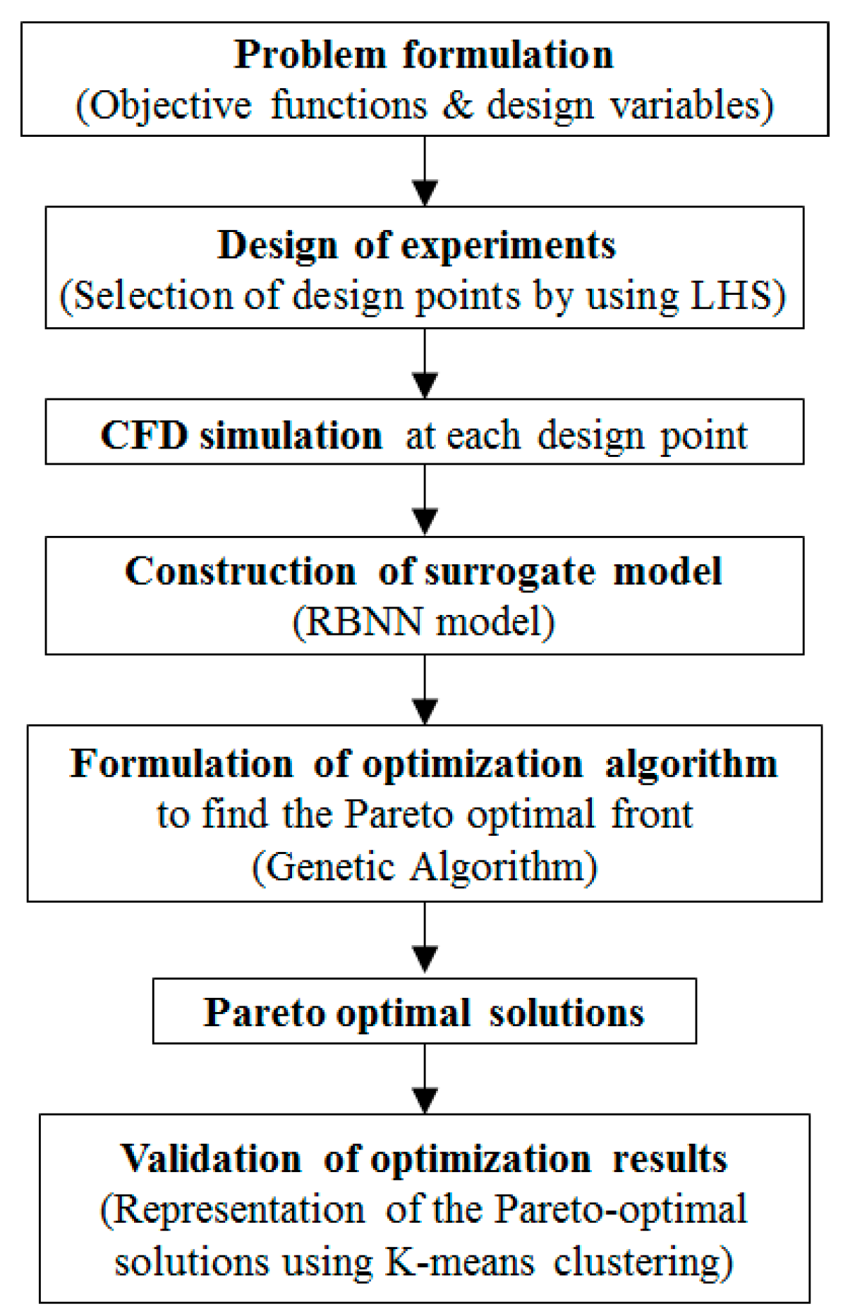
Procedure of multi-objective optimization used in the present work is represented in Figure 3. The first step is selecting design variables and their ranges through a previous parametric study, and the objective functions considering the design goals. The next step is to build the design space using the design of experiments (DOE). In the present work, Latin Hypercube Sampling (LHS) [35] is used as DOE. LHS is an effective sampling technique that uses an m × n simulation matrix where m is the number of levels (sampling points) to be examined and n is the number of design parameters. Each of the n columns of the matrix containing the levels, 1, 2, … , m, is randomly paired to form a Latin hypercube. This approach produces random sample points, ensuring that all of the portions of the design space are represented. Objective function values are calculated by Navier-Stokes analysis at these design points. A surrogate model is constructed to approximate the objective functions based on these objective function values, and MOGA is used to explore global Pareto-optimal solutions in the design space. If the global optimum solution exists in the design space and a termination criterion is satisfied, the multi-objective optimization procedure terminates.
The multi objective optimization problem was formulated, as follows:
where F(x) is an objective function, x is a vector of design variables, and LB and UB denote the vectors of the lower and upper bounds, respectively.
Minimization: F(x) = [F1(x), F2(x), F3(x)… Fn(x)]
Design variable bound: LB ≤ x ≤ UB, x∈ R
In order to obtain LHS design points, MATLAB (MathWorks, Inc., Natick, MA, USA) function ‘lhsdesign’ [36] was used with the criterion ‘maxmin’ (maximize minimum distance between adjacent design point). As a result, uniformly distributed 27 design points were selected for the three design variables in order to construct a surrogate model. The objective function values calculated at these design points by Navier-Stokes analysis are listed in Table 4.
A RBNN model [37] was used to construct surrogate models of the objective functions. The RBNN model contains a two-layered network comprised of a hidden layer of radial neuron and an output layer of linear neuron. The hidden layer executes a nonlinear alteration of the input space to a middle space by using a set of radial basis elements. The output layer then implements a linear combiner to yield the desired targets. The linear model g(x) for the function can be expressed as a linear combination of a set of M radially-symmetric functions, as follows:
where wj is weights and Φj are radial basis functions. Benefit of this surrogate modeling is an ability to reduce computational time owing to the linear nature of the radial basis functions. In the present work, the RBNN function, newrb [36] was used to construct the models. The network training was performed by varying spread constant (SC) to adjust the cross-validation error. In this study, SC1 is related to mixing index, and SC2 is related to pressure drop. The SC values of each objective function were selected through a k-fold cross-validation [38] error test in which the errors were minimum at SC1 = 0.9 and SC2 = 0.5, as shown in Figure 4. The k-fold cross-validation is a validation method to estimate how the results of a statistical analysis generalize to an independent data set.
MOGA was used to find optimal solution on the constructed surrogate model using the MATLAB optimization tool box [36]. MOGA is a randomized global search method that solves functions by imitating progressions observed from natural evolution [37]. Based on the survival and growth of the fittest, MOGA finds new and improved results repeatedly. MOGA describes an initial population of individuals, which represent a part of the solution to the functions. Before the search begins, a series of chromosomes is randomly selected from the design space to obtain the initial population. Through computations, the individuals are selected in a competitive way, based on their fitness functions as measured by each specific objective function. The genetic search operators (i.e., “selection”, “mutation”, and “crossover”) were applied to obtain a next generation of chromosomes, for which the predicted quality of all the chromosomes is better than that of the previous generation. This process is repeated until the termination criterion, which is function tolerance, is met. The following parameters were used: population size = 400, cross over fraction = 0.7, generations = 800, and function tolerance =10−8.
6. Results and Discussion
A grid-dependency test was performed to find out an optimal number of nodes for the spatial discretization of computational space. Four different grid systems with 4.78 × 10⁵ to 1.43 × 10⁶ nodes were tested for development of mixing index along the channel length at two different Reynolds numbers (Re = 1 and 120), as shown in Figure 5. The mixing indices were calculated on the planes perpendicular to the axial direction at four different locations (i.e., start of the main channel, two successive intersection nodes of the crossing channels in X-structure, and the exit). Almost similar profiles of the mixing index development are observed for grid systems with 1.21 × 10⁶ and 1.43 × 10⁶ nodes at both Re = 1 and 120. Hence, grid system with 1.21 × 10⁶ nodes was selected as an optimal grid, commonly at Re = 1 and 120.
The present numerical model was validated in the previous study [25] by both qualitative and quantitative comparisons of the numerical results with the experimental results of Hossain et al. [39], as shown in Figure 6. The optical image of fluid mixing in the first mixing unit at Re = 60 is compared with the numerical result of dye mass fraction distribution on x-y plane located halfway along the channel depth, as shown in Figure 6a. The numerical values of mixing indices at the exit of the micromixer in a Reynolds number range of 0.2–120 are also compared with the experimental data, as shown in Figure 6b. The numerically predicted mixing indices are slightly higher than the experimental data over the whole range. The uncertainties that are involved in the experimental procedures, such as capturing and analyzing experimental image, geometrical variation in fabrication, and wall roughness, can be attributed as the causes for the differences in the mixing indices, as shown in Figure 6b. However, the qualitative and quantitative comparisons between the numerical and experimental results, show acceptable agreements.
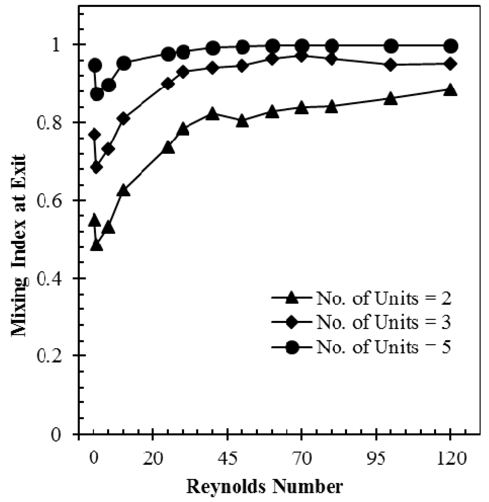
Figure 7 shows effect of number of the mixing units on the mixing performance through a quantitative comparison among the mixing indices at the exits of the micromixers with two, three, and five mixing units at different Reynolds numbers. It is observed that the micromixer with five mixing units exhibits almost complete mixing in most of the Reynolds number range, while the micromixers with two and three mixing units show largely reduced mixing index values over the whole Re range. It is also observed that all the micromixers show minimum mixing indices at Re = 1. Hence, the micromixer with two mixing units was selected in the present work to have more space for enhancement of the mixing performance by optimization.
Effect of Reynolds number on development of mixing index along the axial length of the micromixer (reference design) is shown in Figure 8. The mixing indices were calculated on four y-z planes (at the start of the main channel, the two successive intersection nodes of the crossing channels in X-structure, and the exit) for Reynolds numbers, 1, 20, 40, 80, and 120. The results show that developing rate of mixing index depends on Reynolds number, as shown in Figure 8. The rate of development of mixing index is found to be highest between the first and second intersection nodes at Re = 40.
Following the procedure outlined in Figure 3, Pareto-optimal fronts presenting the optimum trade-off between the two conflicting objectives are plotted, as shown in Figure 9. Pareto-optimal fronts, termed as POF-1 and POF-2 in the Figure 9a,b, respectively, represent two pairs of the objective functions at two different Reynolds numbers: FM at Re = 1 − F∆P at Re = 1 and FM at Re = 120 − F∆P at Re = 120. Concave shape of the Pareto-optimal fronts indicates that an improvement in mixing index occurs with simultaneous increase in pressure drop. Selection of Pareto-optimal solution depends upon the choice of the designer, since each solution is a global Pareto-optimal solution and none of these Pareto-optimal solutions is superior to the others for both objective functions.
In order to analyze the Pareto-optimal solutions, five representative Pareto-optimal designs (PODs) were selected by K-means clustering on each Pareto-optimal front, as shown in Figure 9. PODs A and E at extreme ends of each Pareto-optimal front represent pressure drop-oriented and mixing index-oriented designs, respectively. Accomplishment of one objective function leads to forfeit of the other objective function. At Re = 1, as compared to POD A on POF-1, the mixing index-oriented design, POD E shows a relative enhancement of 34.5 % in the mixing index at the exit. The pressure drop-oriented design, POD A shows a 64.5 % reduction in pressure drop as compared to POD E. Similarly, at Re = 120, POD E shows a relative enhancement of 2.8 % in mixing index at the exit as compared to POD A on POF-2, and POD A shows a 65.7% reduction in pressure drop as compared to POD E. These results reveal that the relative enhancement of mixing index at the exit is much more pronounced at Re = 1 as compared to Re = 120. However, the relative percentage reductions in pressure drop are not much different at both the Reynolds numbers. The higher relative percentage changes in pressure drop than those in mixing index at the exit indicate that mixing index is less sensitive to the design variables as compared to pressure drop.
The results at the representative PODs for POF-1 and POF-2 are listed in Table 5 and Table 6, respectively. It is observed that mixing index at the exit and pressure drop are most sensitive to the design variable, H/W, while w2/Pi remains nearly invariant on POF-1 with the exception of POD A. A high value of mixing index is observed for d/Pi, w2/Pi, and H/W values close to middle of the range, upper bound, and lower bound, respectively. In case of POF-2, the objective functions become more sensitive to the design variables when compared to POF-1. The results of numerical analysis at the PODs shows that maximum enhancements of 18.8% (POD E on POF-1) and 6.0% (POD E on POF-2) in mixing index at the exit are achieved as compared to the reference design at Re = 1 and 120, respectively, by the optimization. Maximum reductions of 5.8% (POD A on POF-1) and 11.1% (POD A on POF-2) in pressure drop are obtained as compared to the reference design at Re = 1 and 120, respectively. The surrogate model predictions of the objective functions values are also compared with the numerical results at the same designs in Table 5 and Table 6. The relative errors of the surrogate predictions for mixing index at the exit and pressure drop are less than 2% and 10%, respectively, at Re = 1, as shown in Table 5. However, these relative errors are increased at Re = 120 to less than 5% and 22%, respectively, as shown in Table 6.
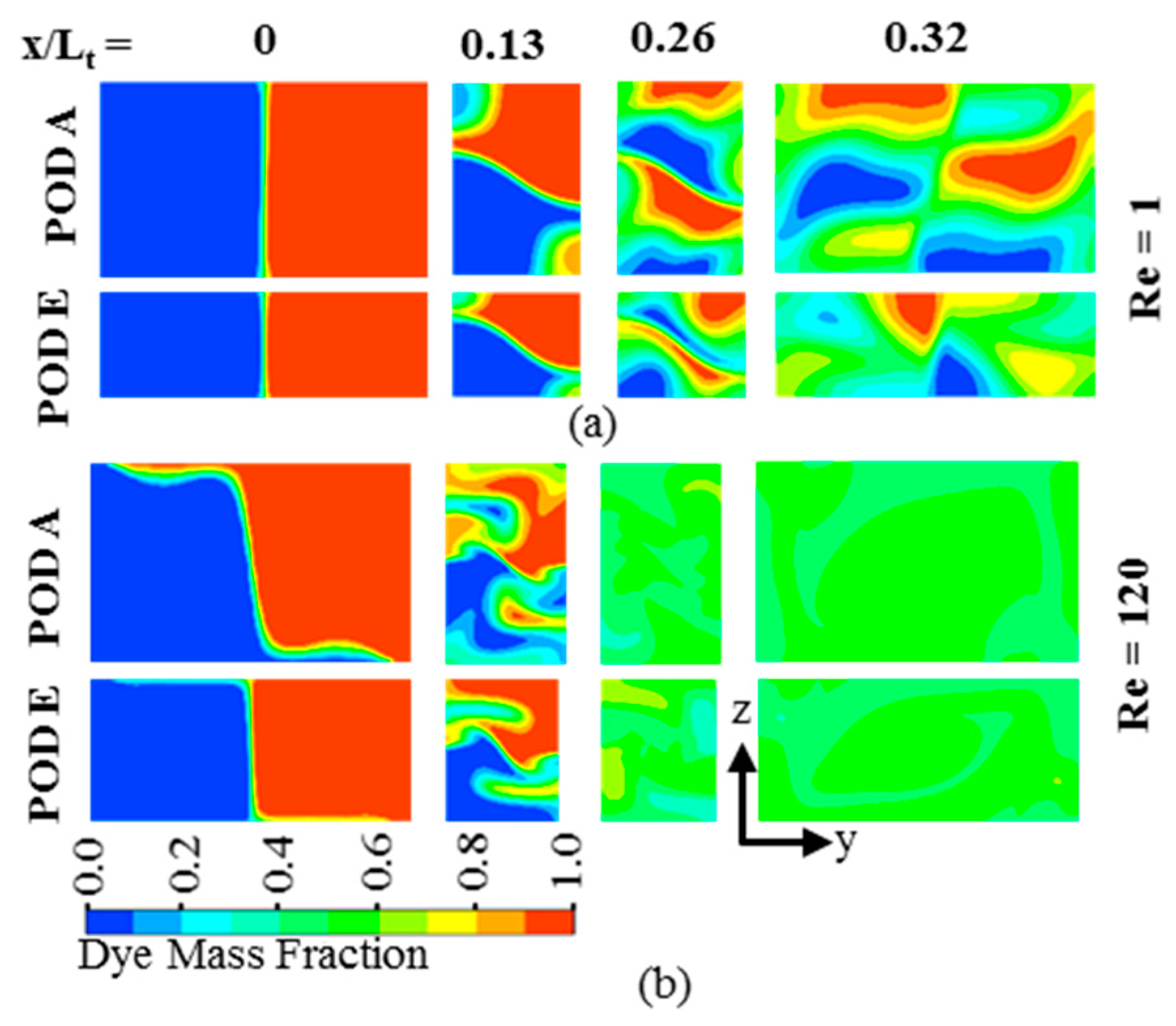
For qualitative comparison of mixings at different PODs on POF-1 (Re = 1) and POF-2 (Re = 120), dye mass fraction contours are plotted on y-z planes at the beginning of the main channel (x/Lt = 0), two successive intersection nodes of the crossing channel in X-structure (x/Lt = 0.13 and 0.26), and the exit (x/Lt = 0.32), respectively, as shown in Figure 10. Two Pareto-optimal designs, i.e. POD A and POD E at the extreme ends of each Pareto-optimal front are selected for the comparison. Number of two-fluid interfaces increases along the channel length for both the PODs. However, there is a distinct difference in the dye mass fraction distribution at the exit of the micromixer between POD A and POD E on POF-1. A more uniform dye mass fraction distribution is observed at the exit for POD E as compared to POD A on POF-1, as shown in Figure 10a, whereas almost similar distributions are observed for POD A and POD E on POF-2 (Figure 10b). This is related to the fact that the change in mixing index along POF-1 (0.439–0.581 in Table 5) is much larger than that along POF-2 (0.936–0.957 in Table 6).
In order to analyze the mixing mechanism, velocity vectors superimposed on the dye mass fraction contours are plotted for POD A and POD E on POF-1 (Re = 1), in Figure 11. It is observed that a saddle-shaped flow structure, which promotes chaotic advection [25], is formed at each intersection node (x/Lt = 0.13 and 0.26) of the crossing microchannels in both of the Pareto-optimal designs, POD A and POD E. However, there is a difference in the fraction of total depth of the microchannel cross-section covered by saddle-shaped pattern between the two designs. In case of POD A, the saddle-shaped flow structure exists only in the middle height of the y-z plane, as shown in Figure 11a. Whereas, in case of POD E, the saddle-shaped flow pattern covers more height of the y-z plane, as shown in Figure 11b. This results in more uniform mass fraction distribution (Figure 11b) and consequently, higher mixing index in POD E, as compared to POD A.
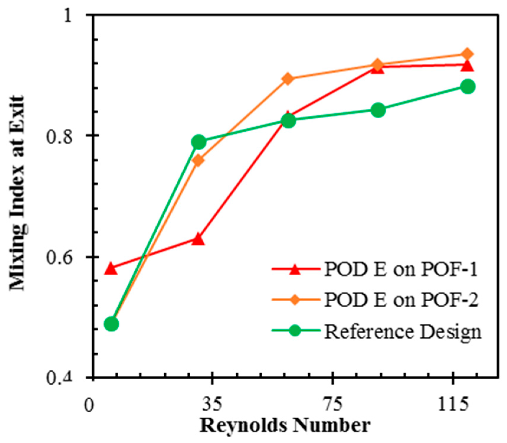
In order to have an idea about the mixing performance of a Pareto-optimal design at Reynolds numbers other than the Reynolds number at which it was obtained, mixing performances of PODs E on POF-1 and POF-2 are compared with the reference design at Reynolds numbers, 1, 30, 60, 90, and 120, as shown in Figure 12. It is observed that POD E on POF-1 shows values of mixing index larger than those of the reference design except at intermediate Reynolds number of 30, but the mixing index values are smaller than those of POD E on POF-2 except at Re = 1. POD E on POF-2 shows improvements in the mixing index at Reynolds numbers larger than 60 when compared to the other designs.
In order to compare the merit of PODs at Re = 1 with previous micromixers, as shown in Table 7, two different mixing performance parameters named, “mixing cost” [40], and “mixing energy cost” (mec) [41] have been used. The terms, “mixing cost” and “mixing energy cost” are defined as:
where η, ΔP, and denote mixing efficiency, pressure drop and mean input power coefficient, respectively. The detail description about these terms can be found in the works of Ortega-Casanova [41,42]. Mixing efficiency (η) and mean input power coefficient () are defined as follows:
where σ, , ΔP, q, ρ, and V are the standard deviation of the concentration, maximum standard deviation, pressure drop, dimensionless flow rate, density of fluid, and average flow velocity, respectively. A micromixer with higher mixing cost and lower mec indicates a more efficient micromixer. From Table 7, it is evident that PODs have neither the best nor the worst values of these parameters. Higher mixing cost values are shown by all of the PODs as compared to the micromixer proposed by Cheri et al. [43]. PODs show higher mec values as compared to the rhombic micromixer with asymmetrical flow [40]. The highest mec value is shown by the micromixer configuration of a rectangular chamber with obstruction proposed by Cheri et al. [43]. Although the micromixer proposed by Cheri et al. [43] shows the highest pressure drop, due to the highest mixing efficiency and the lowest mean input power coefficient, the mec value becomes least.
7. Conclusions
Multi-objective optimizations of a micromixer with 3D serpentine and SAR configuration have been performed at Reynolds numbers, 1 and 120, based on flow and mixing analyses using 3D Navier-Stokes equations and convection-diffusion equation. Three design variables, i.e., d/Pi, w2/Pi, and H/W, were selected, and two objective functions were defined in terms of mixing index at the exit of the micromixer and pressure drop through the micromixer for the optimization. In a parametric study, the mixing index shows maxima for all of the design variables, but the pressure drop shows monotonic variations for all the design variables in the tested ranges. Two concave Pareto-optimal fronts (POF-1 and POF-2) representing trade-off between the two objective functions at Re = 1 and 120, respectively, were obtained by RBNN surrogate model and MOGA. In applying RBNN model, it was found that the k-hold cross-validation errors for mixing index and the pressure drop were minimized with the spread constants, 0.9 and 0.5, respectively. On POF-1 (Re = 1), the preference of a mixing index-oriented design, POD E over a pressure drop-oriented design, POD A leads to 34.5% relative increase in mixing index at the exit, and the preference of POD A over POD E showed 64.5% reduction in pressure drop. On POF-2 (Re = 120), the preference of POD E over POD A leads to only 2.8% relative increase in mixing index at the exit, and the preference of POD A over POD E showed 65.7% reduction in pressure drop. These results indicate that mixing index is less sensitive to the design variables as compared to pressure drop, on the Pareto-optimal fronts. It was found from the numerical analysis at the PODs that the maximum enhancements of 18.8% at POD E on POF-1 and 6.0% at POD E on POF-2 in mixing index at the exit were obtained when compared to the reference design. And, maximum reductions of 5.8% at POD A on POF-1 and 11.1% at POD A on POF-2 in pressure drop were achieved compared to the reference design. Maximum relative error of the surrogate prediction compared to the numerical analysis was smaller for mixing index than pressure drop, and increased with the Reynolds number. In a range of Re = 1–120, POD E on POF-1 showed values of mixing index larger than those of the reference design except at Re = 30, but POD E on POF-2 showed higher mixing performance than the reference design, only for the Reynolds numbers larger than 60.
Acknowledgments
This work was supported by Inha University research grant.
Author Contributions
Wasim Raza performed numerical analysis, analysis of the results, and drafting the manuscript to be submitted, and Sang-Bum Ma performed numerical optimizations. Kwang-Yong Kim revised the manuscript and gave final authorization of the version to be submitted.
Conflicts of Interest
The authors declare there is no conflict of interest.
Nomenclature
| b | length of the vertical sub-channel in O-structure (m) |
| mean input power coefficient | |
| c | mass fraction |
| Dh | hydraulic diameter of the main channel (m) |
| d | spacing between two O-structure (m) |
| F | objective function |
| H | total depth of the channel (m) |
| h1 | depth of the horizontal sub-channel in O-structure (m) |
| h2 | depth of the sub-channel in X-structure (m) |
| Lo | length of initial part of main channel (m) |
| L | total length of the mixing unit (m) |
| Le | length of the channel outlet (m) |
| Lt | total length of the micromixer (m) |
| LHS | Latin hypercube sampling |
| M | mixing index |
| Mo | mixing index at the exit |
| MOGA | multi-objective genetic algorithm |
| N | number of sampling points |
| n | number of mixing units |
| P | pressure (Pa) |
| ΔP | pressure drop (Pa) |
| Pi | pitch length (m) |
| POD | Pareto-optimal design |
| POF | Pareto-optimal front |
| p | length of the horizontal sub-channel in O-structure (m) |
| RBNN | radial basis neural network |
| Re | Reynolds number |
| SAR | split and recombine |
| V | average velocity (m/s) |
| W | width of the main channel (m) |
| w1 | width of the sub-channel in O-structure (m) |
| w2 | width of the sub-channel in X-structure (m) |
| x, y, z | Cartesian coordinates |
| Greek Symbols | |
| α | fluid diffusivity coefficient (m2/s) |
| η | mixing efficiency |
| µ | fluid dynamic viscosity (kg·m−1·s−1) |
| ν | fluid Kinematic viscosity (m2/s) |
| ρ | fluid density (kg/m3) |
| σ | standard deviation |
| Subscripts | |
| i | sampling point or fluid component |
| m | optimal mixing |
| max | maximum value |
| x | axial distance |
References
- Haeberle, S.; Zengerle, R. Microfluidic platforms for lab-on-a-chip applications. Lab Chip 2007, 7, 1094–1110. [Google Scholar] [CrossRef] [PubMed]
- Pagliara, S.; Dettmer, S.L.; Keyser, U.F. Channel-facilitated diffusion boosted by particle binding at the channel entrance. Phys. Rev. Lett. 2014, 113. [Google Scholar] [CrossRef] [PubMed]
- Lee, C.Y.; Wang, W.T.; Liu, C.C.; Fu, L.M. Passive mixers in microfluidic systems: A review. Chem. Eng. J. 2016, 288, 146–160. [Google Scholar] [CrossRef]
- Gossett, D.R.; Weaver, W.M.; MacH, A.J.; Hur, S.C.; Tse, H.T.K.; Lee, W.; Amini, H.; Di Carlo, D. Label-free cell separation and sorting in microfluidic systems. Anal. Bioanal. Chem. 2010, 397, 3249–3267. [Google Scholar] [CrossRef] [PubMed]
- Nguyen, N.-T.; Wu, Z. Micromixers—A review. J. Micromech. Microeng. 2005, 15, R1–R16. [Google Scholar] [CrossRef]
- Hessel, V.; Löwe, H.; Schönfeld, F. Micromixers—A review on passive and active mixing principles. Chem. Eng. Sci. 2005, 60, 2479–2501. [Google Scholar] [CrossRef]
- Capretto, L.; Cheng, W.; Hill, M.; Zhang, X. Micromixing within microfluidic devices. Top. Curr. Chem. 2011, 304, 27–68. [Google Scholar] [PubMed]
- Liu, A.; He, F.; Wang, K.; Zhou, T.; Lu, Y.; Xia, X. Rapid method for design and fabrication of passive micromixers in microfluidic devices using a direct-printing process. Lab Chip 2005, 5, 974–978. [Google Scholar] [CrossRef] [PubMed]
- Kim, D.S.; Lee, S.H.; Kwon, T.H.; Ahn, C.H. A serpentine laminating micromixer combining splitting/recombination and advection. Lab Chip 2005, 5, 739–747. [Google Scholar] [CrossRef] [PubMed]
- Tofteberg, T.; Skolimowski, M.; Andreassen, E.; Geschke, O. A novel passive micromixer: Lamination in a planar channel system. Microfluid. Nanofluid. 2010, 8, 209–215. [Google Scholar] [CrossRef]
- Buchegger, W.; Wagner, C.; Lendl, B.; Kraft, M.; Vellekoop, M.J. A highly uniform lamination micromixer with wedge shaped inlet channels for time resolved infrared spectroscopy. Microfluid. Nanofluid. 2011, 10, 889–897. [Google Scholar] [CrossRef]
- Nimafar, M.; Viktorov, V.; Martinelli, M. Experimental investigation of split and recombination micromixer in confront with basic T- and O- type micromixers. Int. J. Mech. Appl. 2012, 2, 61–69. [Google Scholar] [CrossRef]
- Chen, X.; Shen, J. Numerical analysis of mixing behaviors of two types of E-shape micromixers. Int. J. Heat Mass Transf. 2017, 106, 593–600. [Google Scholar] [CrossRef]
- Liu, R.H.; Stremler, M.A.; Sharp, K.V.; Olsen, M.G.; Santiago, J.G.; Adrian, R.J.; Aref, H.; Beebe, D.J. Passive mixing in a three-dimensional serpentine microchannel. J. Microelectromech. Syst. 2000, 9, 190–197. [Google Scholar] [CrossRef]
- Stroock, A.D.; Dertinger, S.K.W.; Ajdari, A.; Mezic, I.; Stone, H.A.; Whitesides, G.M. Chaotic mixer for microchannels. Science 2002, 295, 647–651. [Google Scholar] [CrossRef] [PubMed]
- Xia, H.M.; Wan, S.Y.M.; Shu, C.; Chew, Y.T. Chaotic micromixers using two-layer crossing channels to exhibit fast mixing at low Reynolds numbers. Lab Chip 2005, 5, 748–755. [Google Scholar] [CrossRef] [PubMed]
- Feng, X.; Ren, Y.; Jiang, H. An effective splitting-and-recombination micromixer with self-rotated contact surface for wide Reynolds number range applications. Biomicrofluidics 2013, 7, 1–10. [Google Scholar] [CrossRef] [PubMed]
- Le The, H.; Le Thanh, H.; Dong, T.; Ta, B.Q.; Tran-Minh, N.; Karlsen, F. An effective passive micromixer with shifted trapezoidal blades using wide Reynolds number range. Chem. Eng. Res. Des. 2015, 93, 1–11. [Google Scholar] [CrossRef]
- Ansari, M.A.; Kim, K.Y. Application of the radial basis neural network to optimization of a micromixer. Chem. Eng. Technol. 2007, 30, 962–966. [Google Scholar] [CrossRef]
- Ansari, M.A.; Kim, K.Y. Shape optimization of a micromixer with staggered herringbone groove. Chem. Eng. Sci. 2007, 62, 6687–6695. [Google Scholar] [CrossRef]
- Kim, B.S.; Kwak, B.S.; Shin, S.; Lee, S.; Kim, K.M.; Jung, H., II; Cho, H.H. Optimization of microscale vortex generators in a microchannel using advanced response surface method. Int. J. Heat Mass Transf. 2011, 54, 118–125. [Google Scholar] [CrossRef]
- Cortes-Quiroz, C.A.; Zangeneh, M.; Goto, A. On multi-objective optimization of geometry of staggered herringbone micromixer. Microfluid. Nanofluid. 2009, 7, 29–43. [Google Scholar] [CrossRef]
- Afzal, A.; Kim, K.Y. Three-objective optimization of a staggered herringbone micromixer. Sens. Actuators B Chem. 2014, 192, 350–360. [Google Scholar] [CrossRef]
- Hossain, S.; Kim, K.-Y. Optimization of a micromixer with two-layer serpentine crossing channels at multiple Reynolds numbers. Chem. Eng. Technol. 2017, 40, 1–10. [Google Scholar] [CrossRef]
- Raza, W.; Hossain, S.; Kim, K.-Y. Effective mixing in a short serpentine split-and-recombination micromixer. Sens. Actuators B Chem. 2018, 258, 381–392. [Google Scholar] [CrossRef]
- Wang, L.; Yang, J.-T. An overlapping crisscross micromixer using chaotic mixing principles. J. Micromech. Microeng. 2006, 16, 2684–2691. [Google Scholar] [CrossRef]
- ANSYS. Solver Theory Guide; CFX-15.0; ANSYS Inc.: Canonsburg, PA, USA, 2013. [Google Scholar]
- Bird, R.B.; Stewart, W.E.; Lightfoot, E.N. Transport Phenomena; John Wiley & Sons: New York, NY, USA, 1960; ISBN 047107392X. [Google Scholar]
- Yang, J.-T.; Huang, K.-J.; Lin, Y.-C. Geometric effects on fluid mixing in passive grooved micromixers. Lab Chip 2005, 5, 1140. [Google Scholar] [CrossRef] [PubMed]
- Chen, X.; Li, T.; Zeng, H.; Hu, Z.; Fu, B. Numerical and experimental investigation on micromixers with serpentine microchannels. Int. J. Heat Mass Transf. 2016, 98, 131–140. [Google Scholar] [CrossRef]
- Kirby, B. Micro- and Nanoscale Fluid Mechanics: Transport in Microfluidic Devices; Cambridge University Press: Cambridge, UK, 2010; ISBN 9780521119030. [Google Scholar]
- Leonard, B.; Mokhtari, S. ULTRA-SHARP Nonoscillatory Convection Schemes for High-Speed Steady Multidimensional Flow; NASA Technical Memorandum; NASA Lewis Research Center: Cleveland, OH, USA, 1990. [Google Scholar]
- Liu, M. Computational study of convective-diffusive mixing in a microchannel mixer. Chem. Eng. Sci. 2011, 66, 2211–2223. [Google Scholar] [CrossRef]
- Boss, J. Evaluation of the homegeneity degree of a mixture. Bulk Solids Handl. 1986, 6, 1207–1215. [Google Scholar]
- McKay, M.D.; Beckman, R.J.; Conover, W.J. Comparison of three methods for selecting values of input variables in the analysis of output from a computer code. Technometrics 1979, 21, 239–245. [Google Scholar]
- MATLAB. The Language of Technical Computing; Release 14. MathWorks, Inc.: Natick, MA, USA, 2004. Available online: http//www.mathworks.com (accessed on 26 November 2017).
- Orr, M. Introduction to radial basis function networks. Univ. Edinbg. 1996, 1–7. [Google Scholar] [CrossRef]
- Stone, M. Cross-validatory choice and assessment of statistical predictions. J. R. Stat. Soc. 1974, 36, 111–147. [Google Scholar]
- Hossain, S.; Lee, I.; Kim, S.M.; Kim, K.-Y. A micromixer with two-layer serpentine crossing channels having excellent mixing performance at low Reynolds numbers. Chem. Eng. J. 2017, 327, 268–277. [Google Scholar] [CrossRef]
- Chung, C.K.; Shih, T.R. A rhombic micromixer with asymmetrical flow for enhancing mixing. J. Micromech. Microeng. 2007, 17, 2495. [Google Scholar] [CrossRef]
- Ortega-Casanova, J. CFD study on mixing enhancement in a channel at a low reynolds number by pitching a square cylinder. Comput. Fluids 2017, 145, 141–152. [Google Scholar] [CrossRef]
- Ortega-Casanova, J. Enhancing mixing at a very low Reynolds number by a heaving square cylinder. J. Fluids Struct. 2016, 65, 1–20. [Google Scholar] [CrossRef]
- Sadegh Cheri, M.; Latifi, H.; Salehi Moghaddam, M.; Shahraki, H. Simulation and experimental investigation of planar micromixers with short-mixing-length. Chem. Eng. J. 2013, 234, 247–255. [Google Scholar] [CrossRef]
Figure 1.
Geometry of micromixer with OX- shaped units: (a) planar view [25]; and, (b) three-dimensional (3D) view.
Figure 1.
Geometry of micromixer with OX- shaped units: (a) planar view [25]; and, (b) three-dimensional (3D) view.
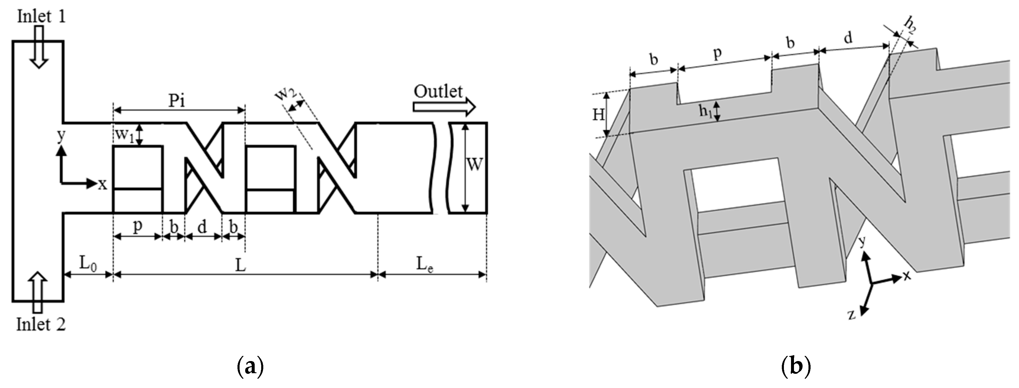
Figure 2.
Effects of design variables on objective functions at Re = 1: (a) mixing index at the exit; and, (b) pressure drop.
Figure 2.
Effects of design variables on objective functions at Re = 1: (a) mixing index at the exit; and, (b) pressure drop.
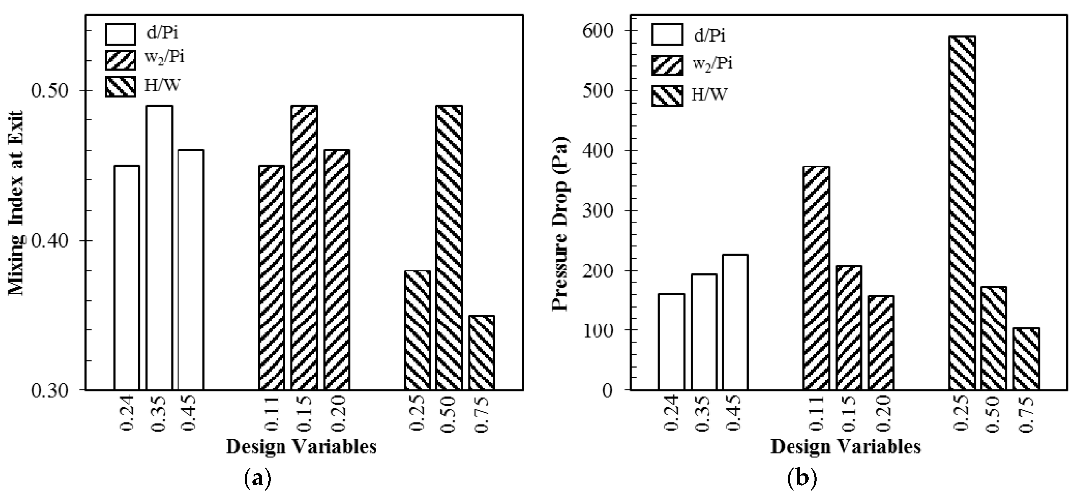
Figure 3.
Multi-objective optimization procedure.

Figure 4.
Cross-validation error vs. spread constant (SC) for the objective functions: (a) Mixing index (SC1); (b) Zoomed in view of encircled area in Figure 4a; (c) Pressure drop (SC2); (d) Zoomed in view of encircled area in Figure 4c.
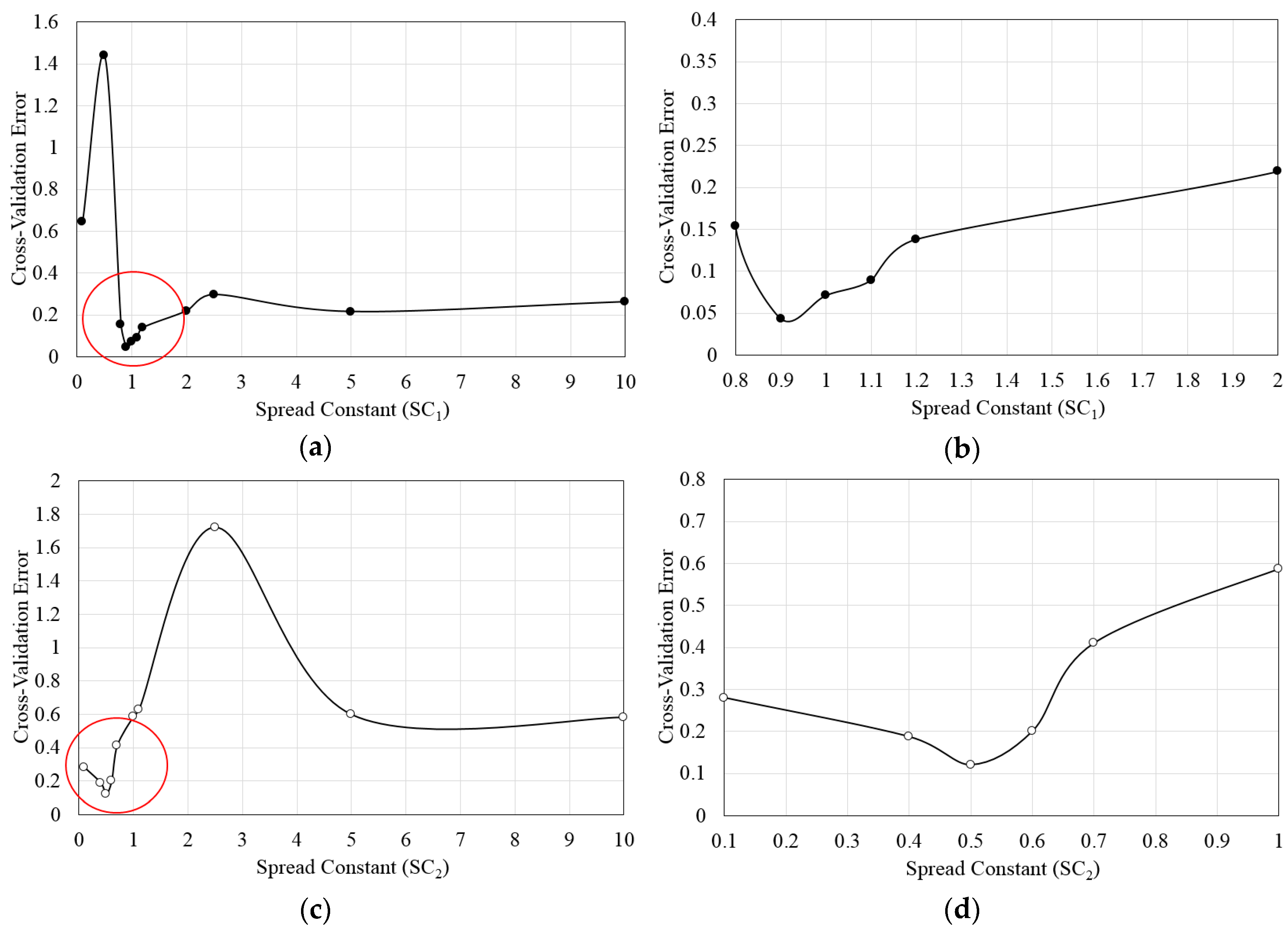
Figure 5.
Grid-dependency tests for mixing index development along axial length of the reference design: (a) Re = 1; and, (b) Re = 120.
Figure 5.
Grid-dependency tests for mixing index development along axial length of the reference design: (a) Re = 1; and, (b) Re = 120.
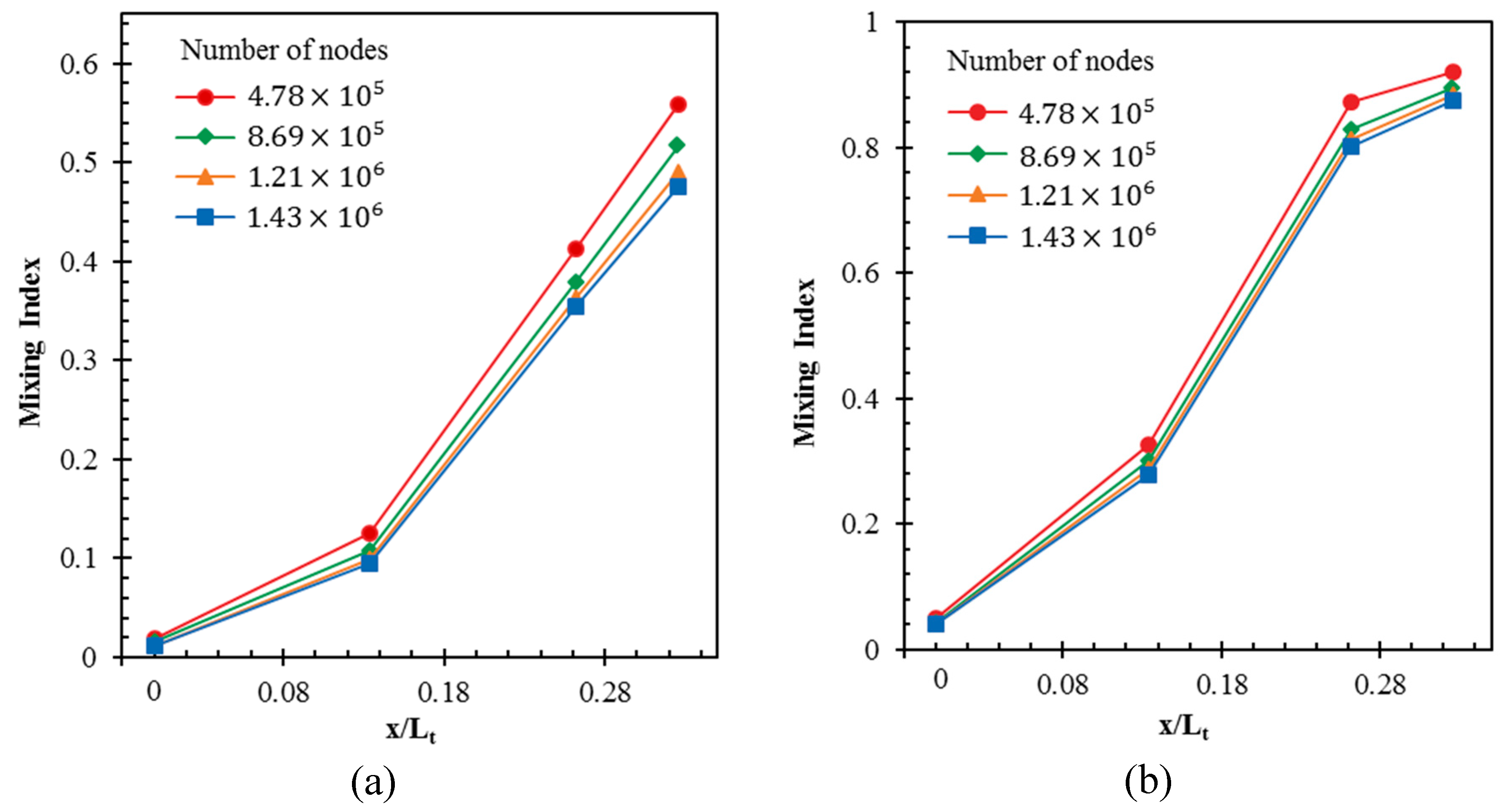
Figure 6.
Validation of numerical results compared with experimental data [25]: (a) qualitative comparison of dye mass fraction distribution on x-y plane located halfway along the channel depth between experiment and numerical analysis at Re = 60; and, (b) quantitative comparison of mixing indices at the exit for different Reynolds numbers between experiment and numerical analysis.
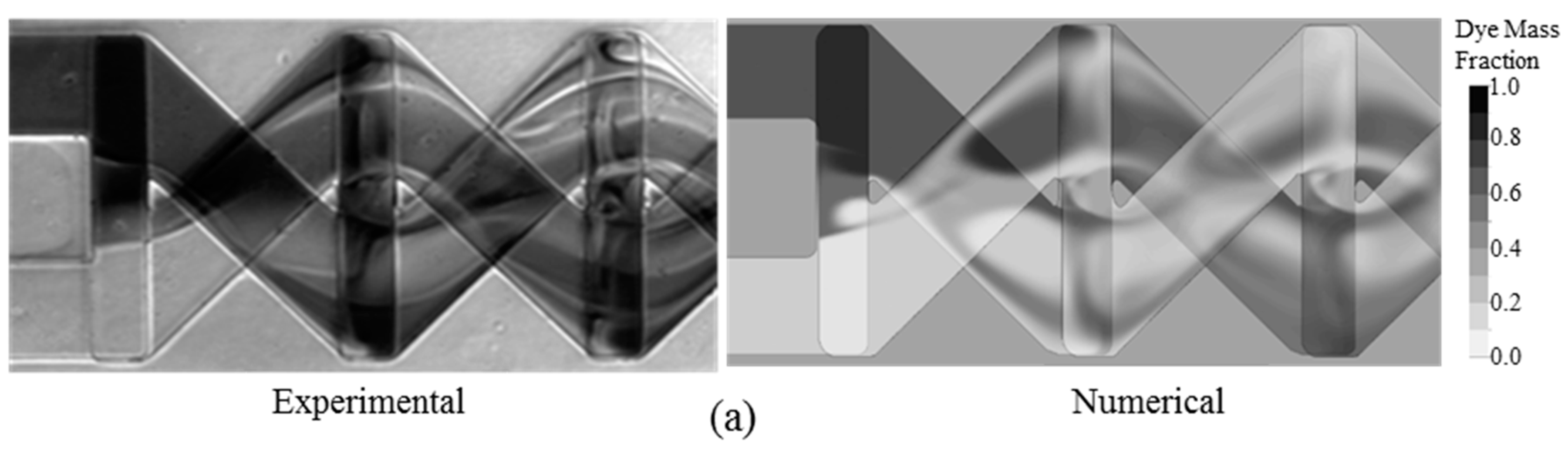
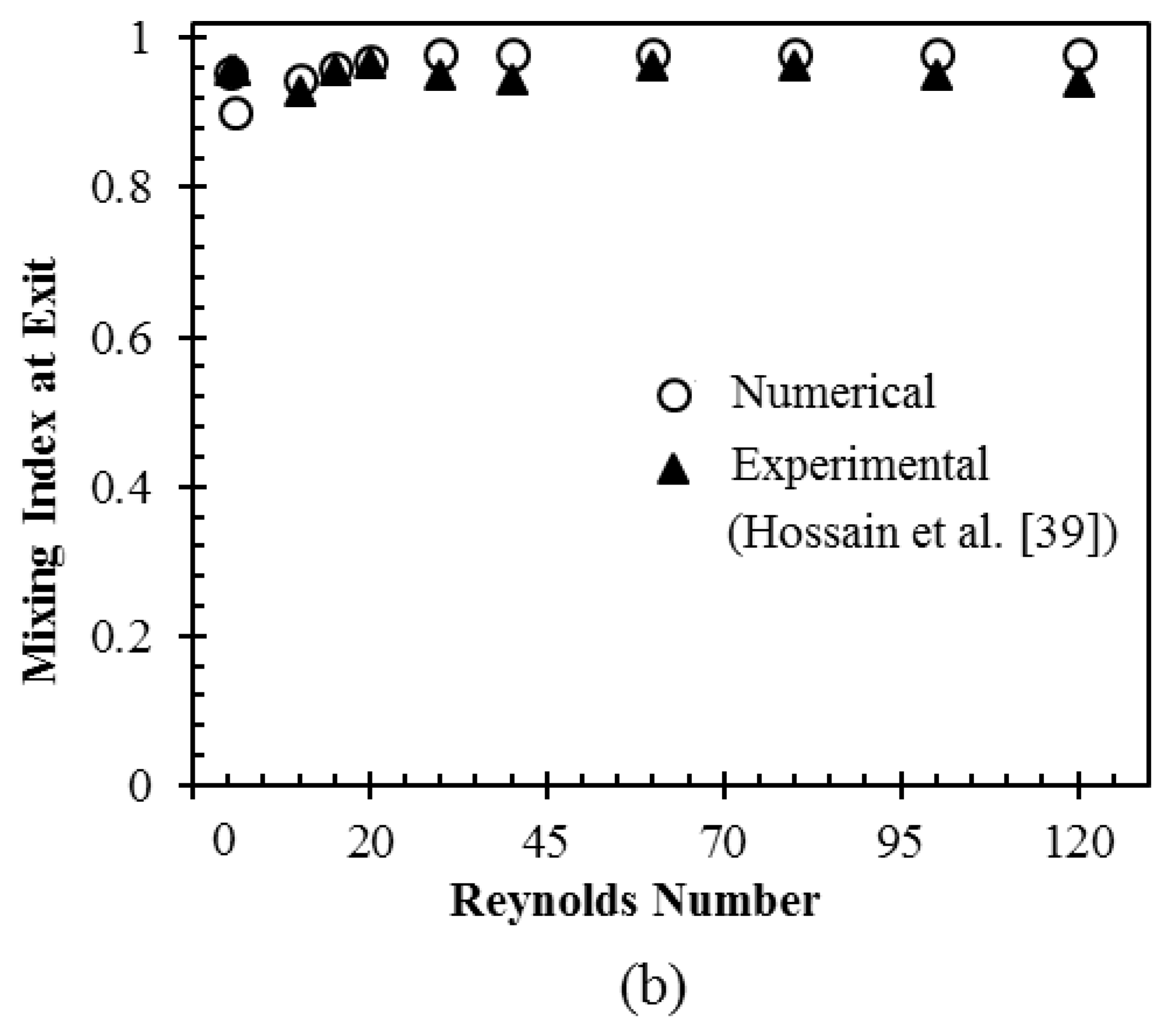
Figure 7.
Variations of mixing index at the exit with Reynolds number for three different numbers of mixing units.
Figure 7.
Variations of mixing index at the exit with Reynolds number for three different numbers of mixing units.

Figure 8.
Developments of mixing index along the axial length of micromixer (reference design) for different Reynolds numbers.
Figure 8.
Developments of mixing index along the axial length of micromixer (reference design) for different Reynolds numbers.

Figure 9.
Pareto-optimal fronts: (a) mixing index at Re = 1 vs. pressure drop at Re = 1; and (b) mixing index at Re = 120 vs. pressure drop at Re = 120.
Figure 9.
Pareto-optimal fronts: (a) mixing index at Re = 1 vs. pressure drop at Re = 1; and (b) mixing index at Re = 120 vs. pressure drop at Re = 120.
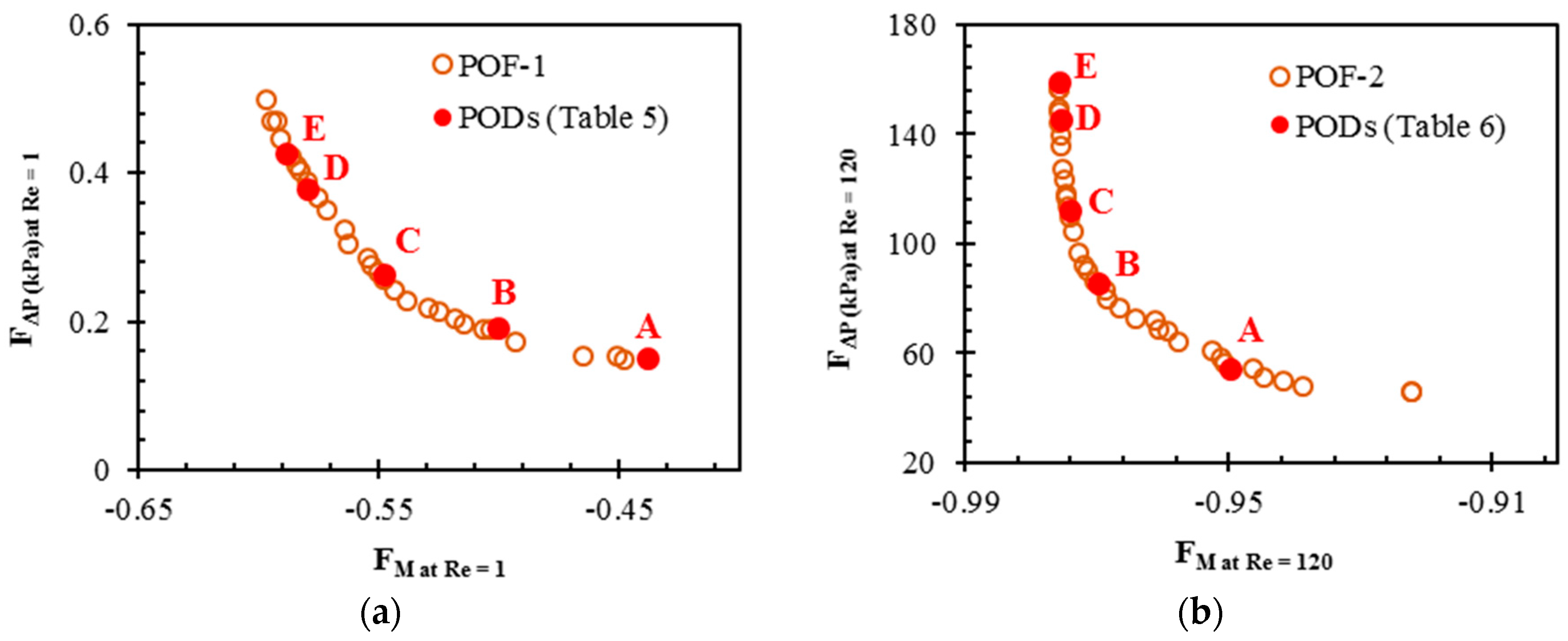
Figure 10.
Dye mass fraction distributions on y-z planes for POD A and POD E: (a) Pareto-optimal fronts (POF)-1 (Re = 1); and (b) POF-2 (Re = 120).
Figure 10.
Dye mass fraction distributions on y-z planes for POD A and POD E: (a) Pareto-optimal fronts (POF)-1 (Re = 1); and (b) POF-2 (Re = 120).

Figure 11.
Velocity vectors and concentration contours on y-z planes at first (x/Lt = 0.13) and second (x/Lt=0.26) X-structure intersection nodes: (a) POD A; and, (b) POD E, on POF-1.
Figure 11.
Velocity vectors and concentration contours on y-z planes at first (x/Lt = 0.13) and second (x/Lt=0.26) X-structure intersection nodes: (a) POD A; and, (b) POD E, on POF-1.
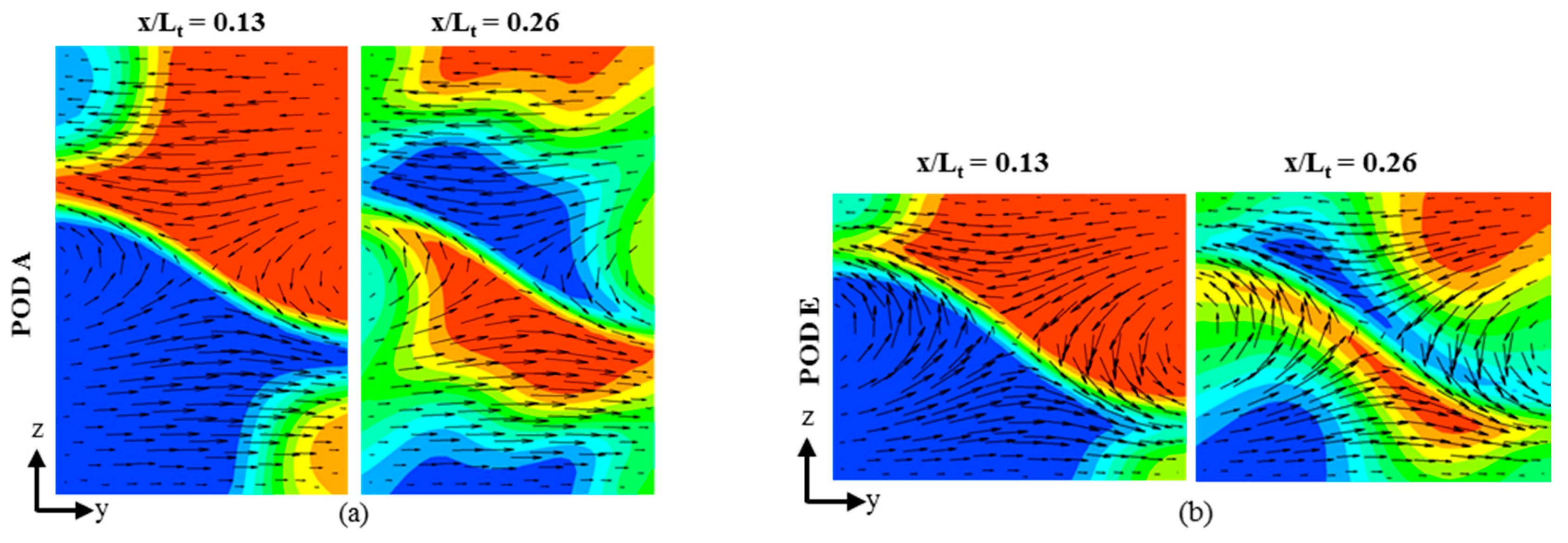
Figure 12.
Variations of mixing index at the exit with Reynolds number for POD E on POF-1, POD E on POF-2, and reference design.
Figure 12.
Variations of mixing index at the exit with Reynolds number for POD E on POF-1, POD E on POF-2, and reference design.

Table 1.
Geometric parameters and their values.
| Geometric Parameter | Value (In µm) |
|---|---|
| Length of initial part of main channel, L0 | 100 |
| Exit channel length, Le | 1500 |
| Total length, Lt | 2150 |
| Pitch length, Pi | 275 |
| Width of main channel, W | 200 |
| Width of O-structure, w1 | 50 |
| Width of X-structure, w2 | 50 |
| Distance between O-structures, d | 75 |
| Depth of horizontal portion of O-structure, h1 | 50 |
| Depth of X-structure, h2 | 50 |
| Total depth of main channel, H | 100 |
Table 2.
Design variables and their ranges.
| Design Variables | Lower Limit | Upper Limit |
|---|---|---|
| d/Pi | 0.236 | 0.455 |
| w2/Pi | 0.109 | 0.200 |
| H/W | 0.250 | 0.750 |
Table 3.
Reference design and its objective functions values.
| Reference Design | ||||||
|---|---|---|---|---|---|---|
| Design Variables | Objective Functions | |||||
| d/Pi | w2/Pi | H/W | Mixing Index at exit, M0 | Pressure drop, ΔP (kPa) | ||
| Re = 1 | Re = 120 | Re = 1 | Re = 120 | |||
| 0.272 | 0.182 | 0.500 | 0.489 | 0.883 | 0.171 | 69.741 |
Table 4.
Design variables and objective function values at Latin hypercube sampling (LHS) design points.
Table 4.
Design variables and objective function values at Latin hypercube sampling (LHS) design points.
| Design Point | Design Variables | Objective Functions (Re = 1) | Objective Functions (Re = 120) | ||||
|---|---|---|---|---|---|---|---|
| d/Pi | w2/Pi | H/W | Mixing Index, Mo | Pressure Drop, ∆P (kPa) | Mixing Index, Mo | Pressure Drop, ∆P (kPa) | |
| 1 | 0.377 | 0.162 | 0.635 | 0.410 | 0.962 | 0.171 | 61.976 |
| 2 | 0.418 | 0.197 | 0.673 | 0.400 | 0.926 | 0.136 | 48.443 |
| 3 | 0.369 | 0.172 | 0.442 | 0.504 | 0.962 | 0.254 | 91.358 |
| 4 | 0.288 | 0.169 | 0.423 | 0.539 | 0.929 | 0.248 | 98.528 |
| 5 | 0.442 | 0.141 | 0.577 | 0.404 | 0.854 | 0.261 | 89.404 |
| 6 | 0.272 | 0.131 | 0.731 | 0.374 | 0.977 | 0.171 | 69.802 |
| 7 | 0.385 | 0.113 | 0.500 | 0.419 | 0.750 | 0.422 | 153.596 |
| 8 | 0.434 | 0.148 | 0.385 | 0.488 | 0.795 | 0.422 | 143.310 |
| 9 | 0.321 | 0.155 | 0.712 | 0.391 | 0.915 | 0.123 | 46.962 |
| 10 | 0.329 | 0.183 | 0.692 | 0.382 | 0.930 | 0.232 | 86.091 |
| 11 | 0.345 | 0.127 | 0.654 | 0.371 | 0.847 | 0.334 | 114.287 |
| 12 | 0.426 | 0.117 | 0.615 | 0.468 | 0.920 | 0.350 | 151.380 |
| 13 | 0.280 | 0.120 | 0.462 | 0.474 | 0.972 | 0.234 | 88.623 |
| 14 | 0.345 | 0.155 | 0.500 | 0.472 | 0.935 | 0.192 | 68.240 |
| 15 | 0.402 | 0.186 | 0.519 | 0.472 | 0.935 | 0.192 | 68.240 |
| 16 | 0.256 | 0.190 | 0.365 | 0.459 | 0.862 | 0.266 | 105.153 |
| 17 | 0.337 | 0.179 | 0.327 | 0.580 | 0.914 | 0.391 | 136.554 |
| 18 | 0.353 | 0.124 | 0.288 | 0.495 | 0.831 | 0.810 | 300.789 |
| 19 | 0.361 | 0.152 | 0.269 | 0.572 | 0.852 | 0.715 | 247.365 |
| 20 | 0.248 | 0.158 | 0.596 | 0.450 | 0.885 | 0.150 | 65.947 |
| 21 | 0.297 | 0.193 | 0.481 | 0.499 | 0.888 | 0.178 | 68.949 |
| 22 | 0.410 | 0.176 | 0.250 | 0.541 | 0.818 | 0.754 | 229.751 |
| 23 | 0.240 | 0.165 | 0.404 | 0.543 | 0.915 | 0.248 | 108.789 |
| 24 | 0.393 | 0.138 | 0.558 | 0.420 | 0.891 | 0.261 | 93.075 |
| 25 | 0.313 | 0.134 | 0.538 | 0.448 | 0.933 | 0.250 | 99.692 |
| 26 | 0.264 | 0.110 | 0.308 | 0.493 | 0.941 | 0.736 | 342.159 |
| 27 | 0.305 | 0.145 | 0.346 | 0.534 | 0.911 | 0.432 | 173.488 |
Table 5.
Results of optimization at representative Pareto-optimal designs (PODs) for Re = 1.
| Selected PODs | Design Variables | Surrogate Prediction | Numerical Analysis | % Error | |||||
|---|---|---|---|---|---|---|---|---|---|
| d/Pi | w2/Pi | H/W | Mo | ΔP (kPa) | Mo | ΔP (kPa) | Mo | ΔP | |
| A | 0.308 | 0.163 | 0.602 | 0.438 | 0.152 | 0.439 | 0.161 | −0.23 | −5.59 |
| B | 0.296 | 0.171 | 0.485 | 0.500 | 0.190 | 0.498 | 0.199 | 0.40 | −4.52 |
| C | 0.318 | 0.175 | 0.404 | 0.548 | 0.265 | 0.551 | 0.269 | −0.54 | −1.49 |
| D | 0.327 | 0.175 | 0.338 | 0.580 | 0.378 | 0.587 | 0.373 | −1.19 | 1.34 |
| E | 0.330 | 0.176 | 0.328 | 0.589 | 0.428 | 0.581 | 0.391 | 1.38 | 9.46 |
Table 6.
Results of optimization at representative PODs for Re = 120.
| Selected PODs | Design Variables | Surrogate Prediction | Numerical Analysis | % Error | |||||
|---|---|---|---|---|---|---|---|---|---|
| d/Pi | w2/Pi | H/W | Mo | ΔP (kPa) | Mo | ΔP (kPa) | Mo | ΔP | |
| A | 0.329 | 0.161 | 0.628 | 0.950 | 54.544 | 0.957 | 61.966 | −0.73 | −11.98 |
| B | 0.272 | 0.132 | 0.583 | 0.970 | 85.442 | 0.951 | 92.696 | 2.00 | −7.83 |
| C | 0.254 | 0.123 | 0.472 | 0.974 | 112.168 | 0.936 | 142.565 | 4.06 | −21.32 |
| D | 0.245 | 0.120 | 0.464 | 0.976 | 145.752 | 0.948 | 154.631 | 2.95 | −5.74 |
| E | 0.241 | 0.120 | 0.446 | 0.976 | 158.992 | 0.936 | 166.768 | 4.27 | −4.66 |
Table 7.
Comparison of mixing cost and mixing energy cost of PODs on POF-1 with previous micromixers.
Table 7.
Comparison of mixing cost and mixing energy cost of PODs on POF-1 with previous micromixers.
| Previous Works | |||||||||
|---|---|---|---|---|---|---|---|---|---|
| PODs on POF-1 | Ortega-Casanova [41] | Ortega-Casanova [42] | Chung and Shih [40] | Cheri et al. [43] | |||||
| Parameters | A | B | C | D | E | ||||
| η | 44 | 50 | 55 | 59 | 58 | 27 | 27 | 55 | 60 |
| ΔP (Pa) | 161 | 199 | 269 | 373 | 391 | -* | -* | 162 | 530 |
| 7273 | 6800 | 7141 | 7619 | 7624 | 904 | 550 | 10,000 | 100 | |
| mixing cost | 0.273 | 0.251 | 0.205 | 0.157 | 0.149 | -* | -* | 0.3 | 0.113 |
| mec | 166 | 137 | 130 | 130 | 131 | 33 | 20 | 182 | 1.6 |
-* denotes data not available.
© 2018 by the authors. Licensee MDPI, Basel, Switzerland. This article is an open access article distributed under the terms and conditions of the Creative Commons Attribution (CC BY) license (http://creativecommons.org/licenses/by/4.0/).
Share and Cite
MDPI and ACS Style
Raza, W.; Ma, S.-B.; Kim, K.-Y. Multi-Objective Optimizations of a Serpentine Micromixer with Crossing Channels at Low and High Reynolds Numbers. Micromachines 2018, 9, 110. https://doi.org/10.3390/mi9030110
AMA Style
Raza W, Ma S-B, Kim K-Y. Multi-Objective Optimizations of a Serpentine Micromixer with Crossing Channels at Low and High Reynolds Numbers. Micromachines. 2018; 9(3):110. https://doi.org/10.3390/mi9030110
Chicago/Turabian StyleRaza, Wasim, Sang-Bum Ma, and Kwang-Yong Kim. 2018. "Multi-Objective Optimizations of a Serpentine Micromixer with Crossing Channels at Low and High Reynolds Numbers" Micromachines 9, no. 3: 110. https://doi.org/10.3390/mi9030110
Note that from the first issue of 2016, this journal uses article numbers instead of page numbers. See further details here.