Experimental Assessment of Color Deconvolution and Color Normalization for Automated Classification of Histology Images Stained with Hematoxylin and Eosin


Abstract
:Simple Summary
Abstract
1. Introduction
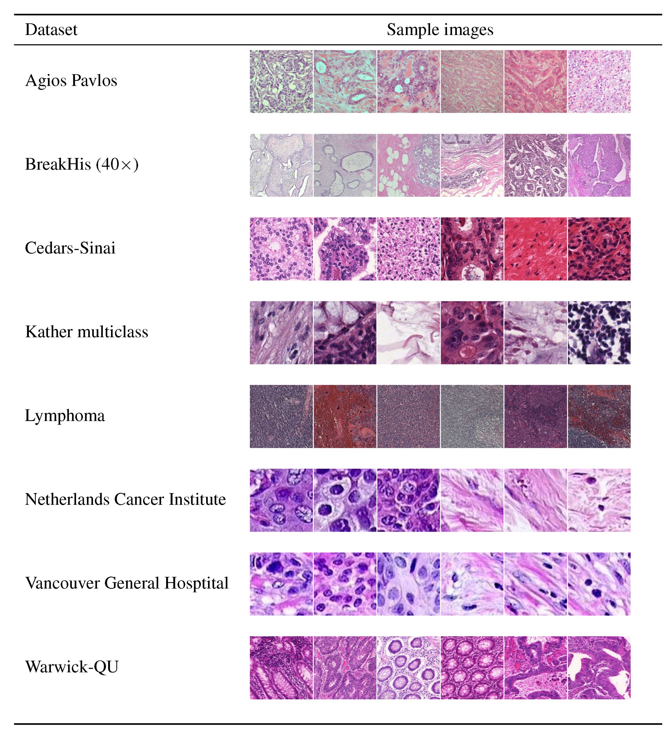
2. Materials
2.1. Agios Pavlos (AP)
2.2. BreakHis (BH)
2.3. Cedars-Sinai (CS)
2.4. HICL
2.5. Kather Multiclass (KM)
2.6. Lymphoma
2.7. Netherlands Cancer Institute (NKI)
2.8. Vancouver General Hospital (VGH)
2.9. Warwick-QU (WR)
2.10. Combined Datasets (AP+HICL, NKI+VGH)
3. Methods
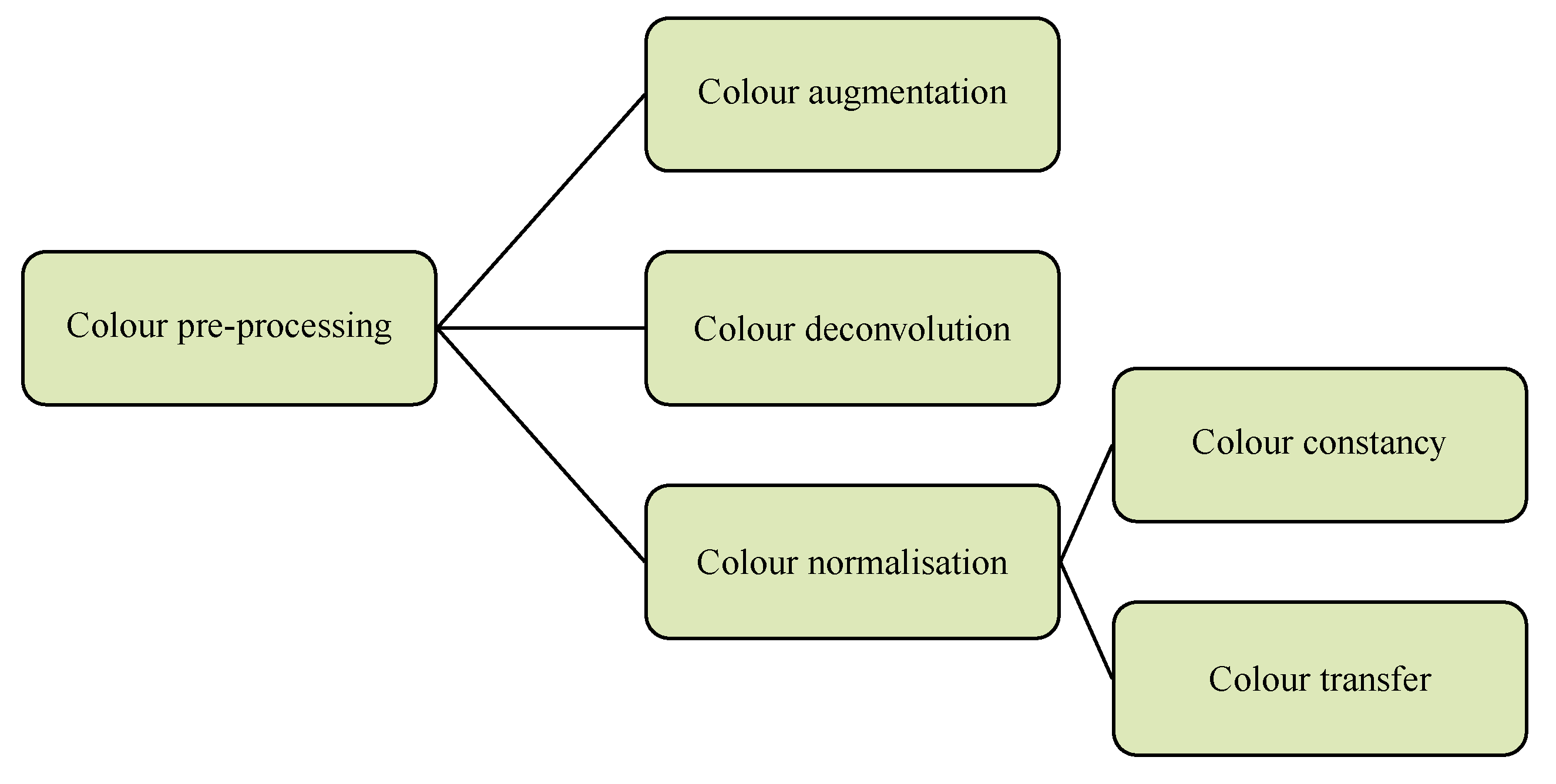
3.1. Color Pre-Processing
3.1.1. Color Augmentation
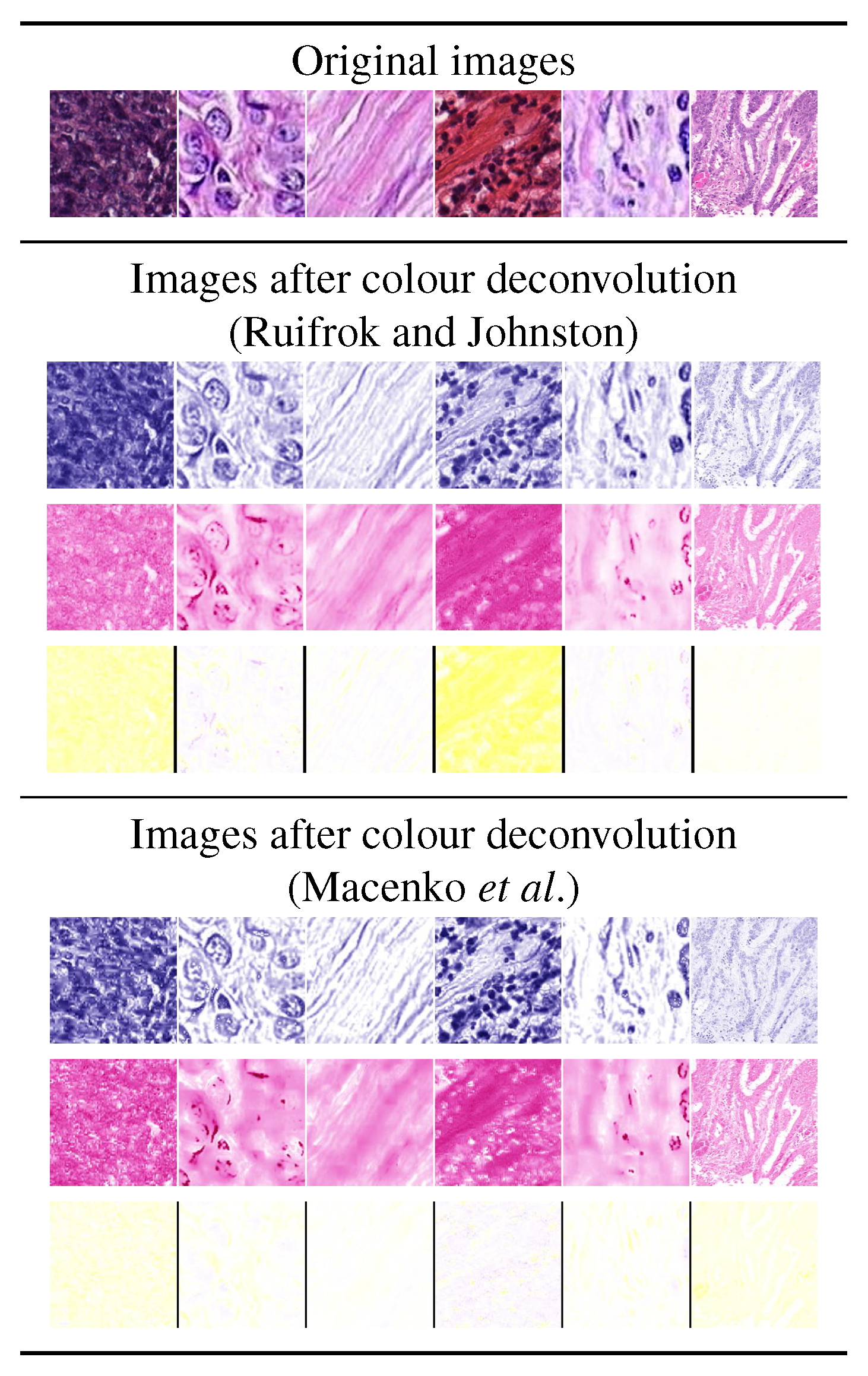
3.1.2. Color Deconvolution
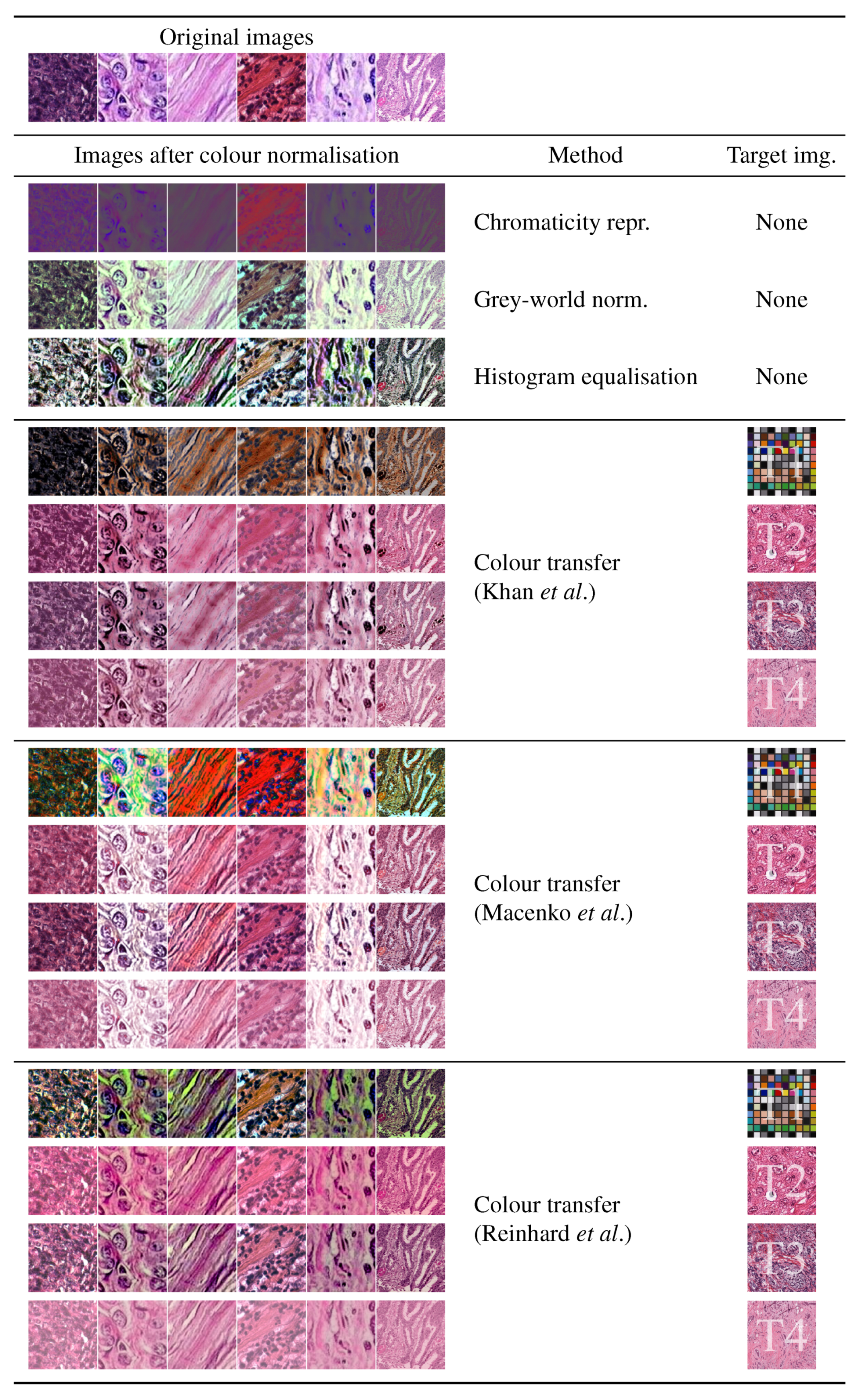
3.1.3. Colour Normalization
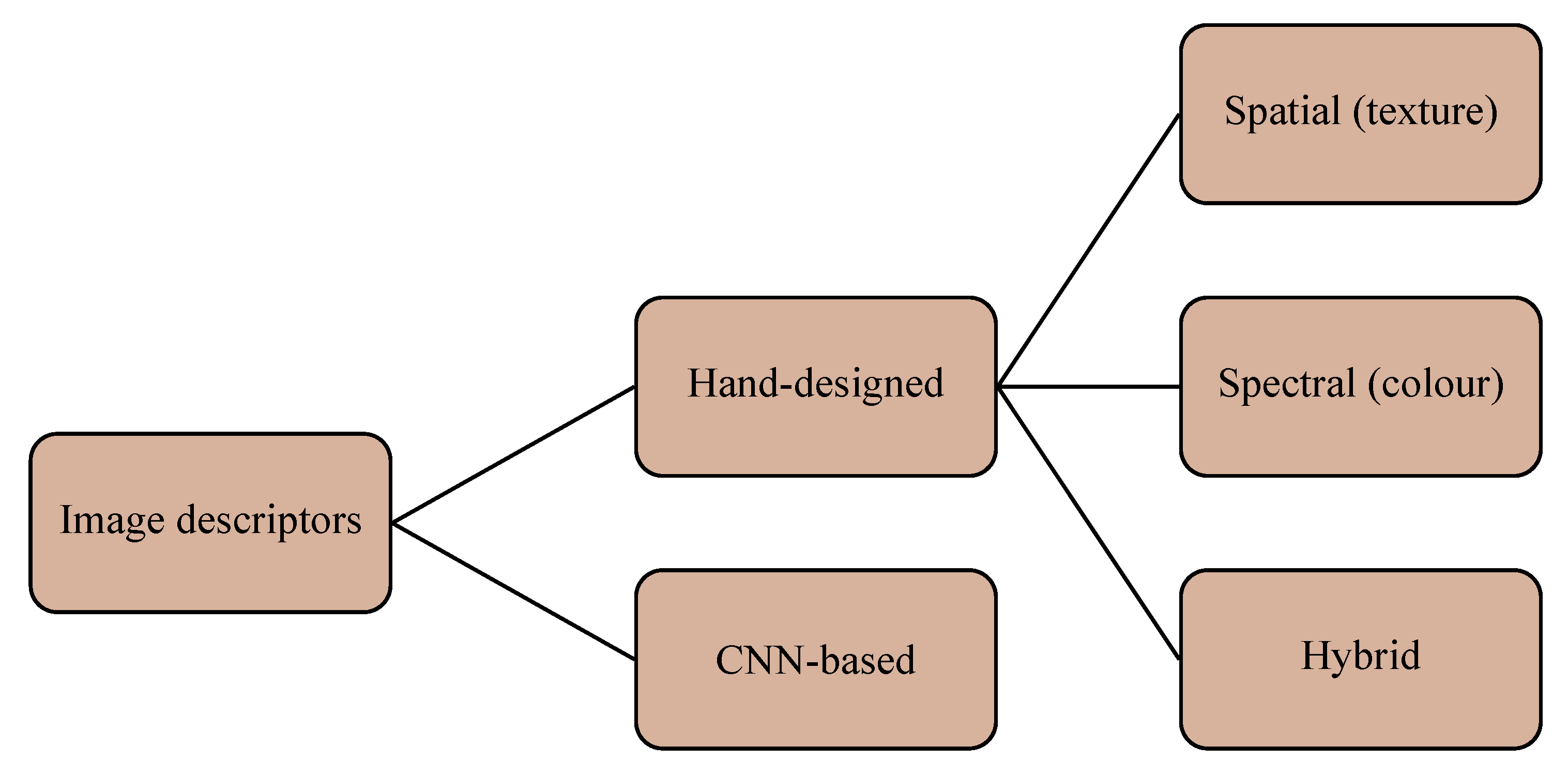
3.2. Image Descriptors
3.2.1. Hand-Designed Methods (Spectral)
Three-Dimensional Color Histogram (FullHist)
One-Dimensional Marginal Color Histograms (MargHists)
3.2.2. Hand-Designed Methods (Spatial)
Grey-Level Co-Occurrence Matrices (GLCM)
Gabor Filters (Gabor)
Local Binary Patterns (LBP)
3.2.3. Hand-Designed Methods (Hybrid)
3.2.4. Pre-Trained Convolutional Networks
3.3. Further Pre-Processing Steps
4. Experiments
5. Results and Discussion
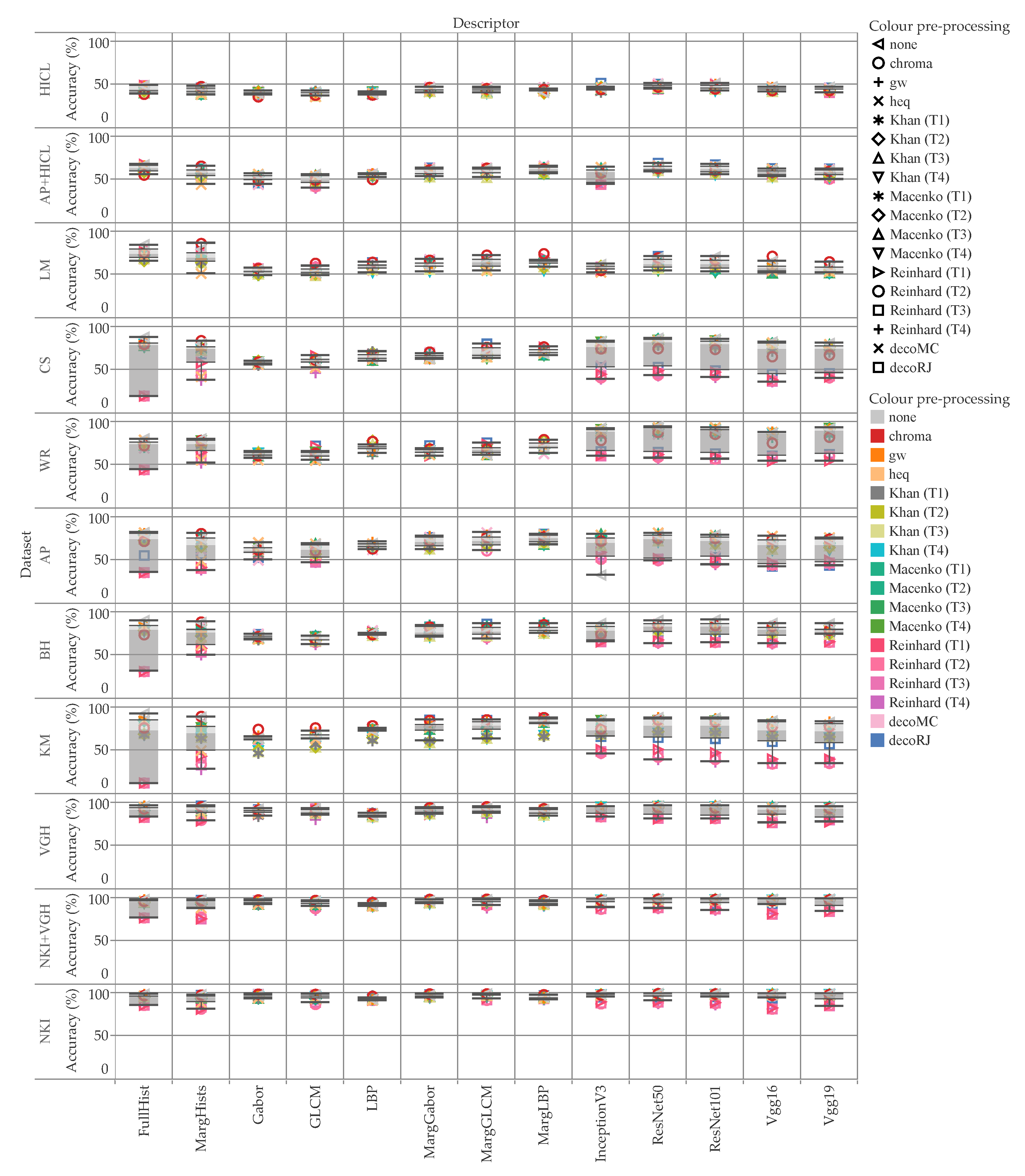
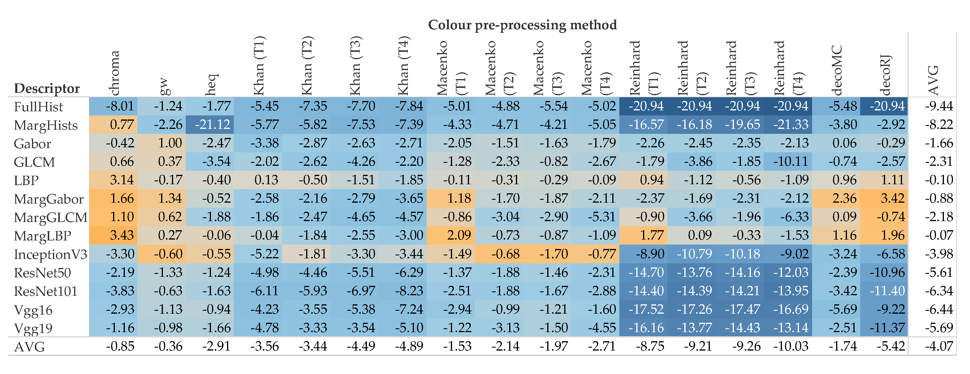
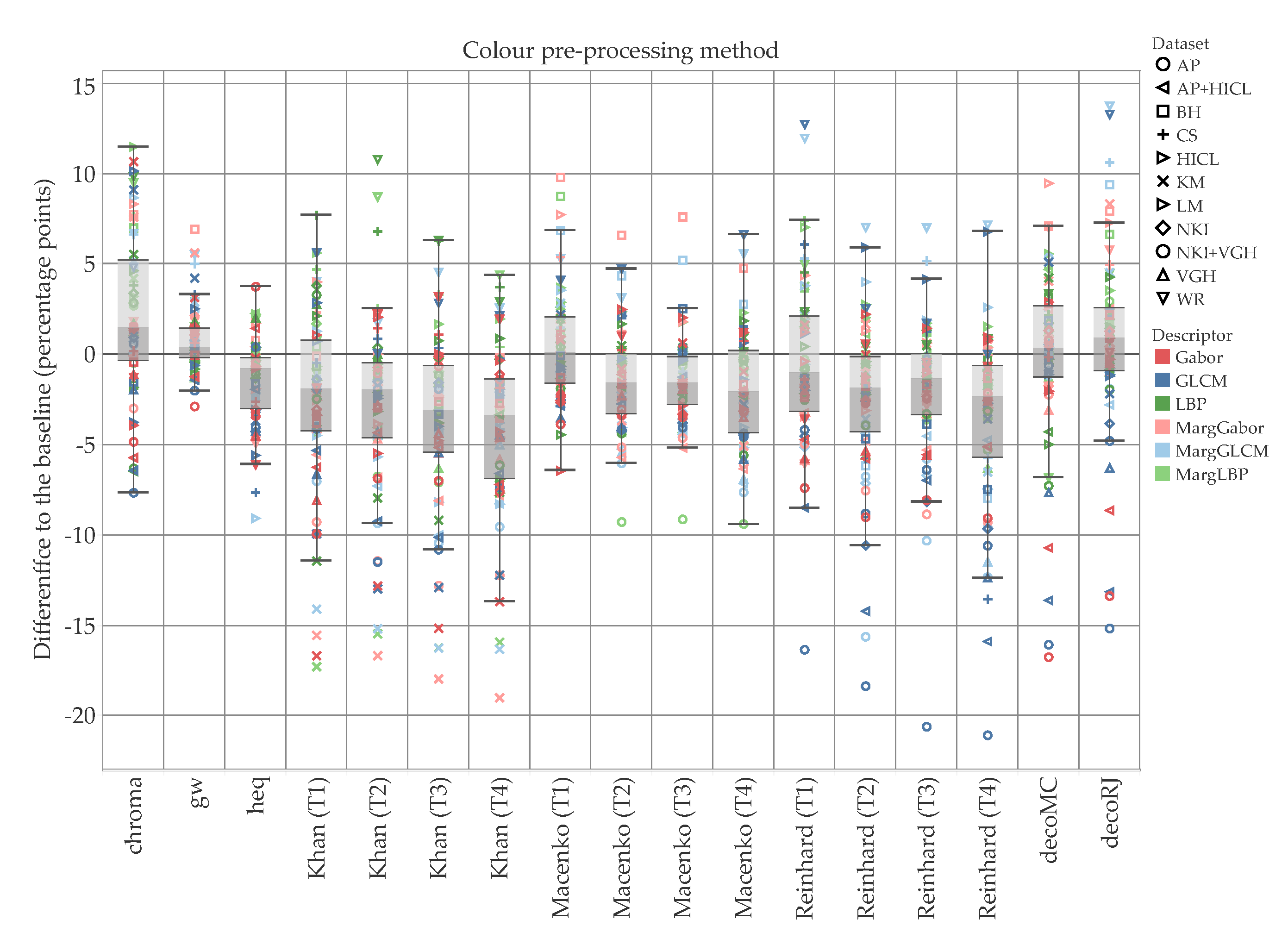
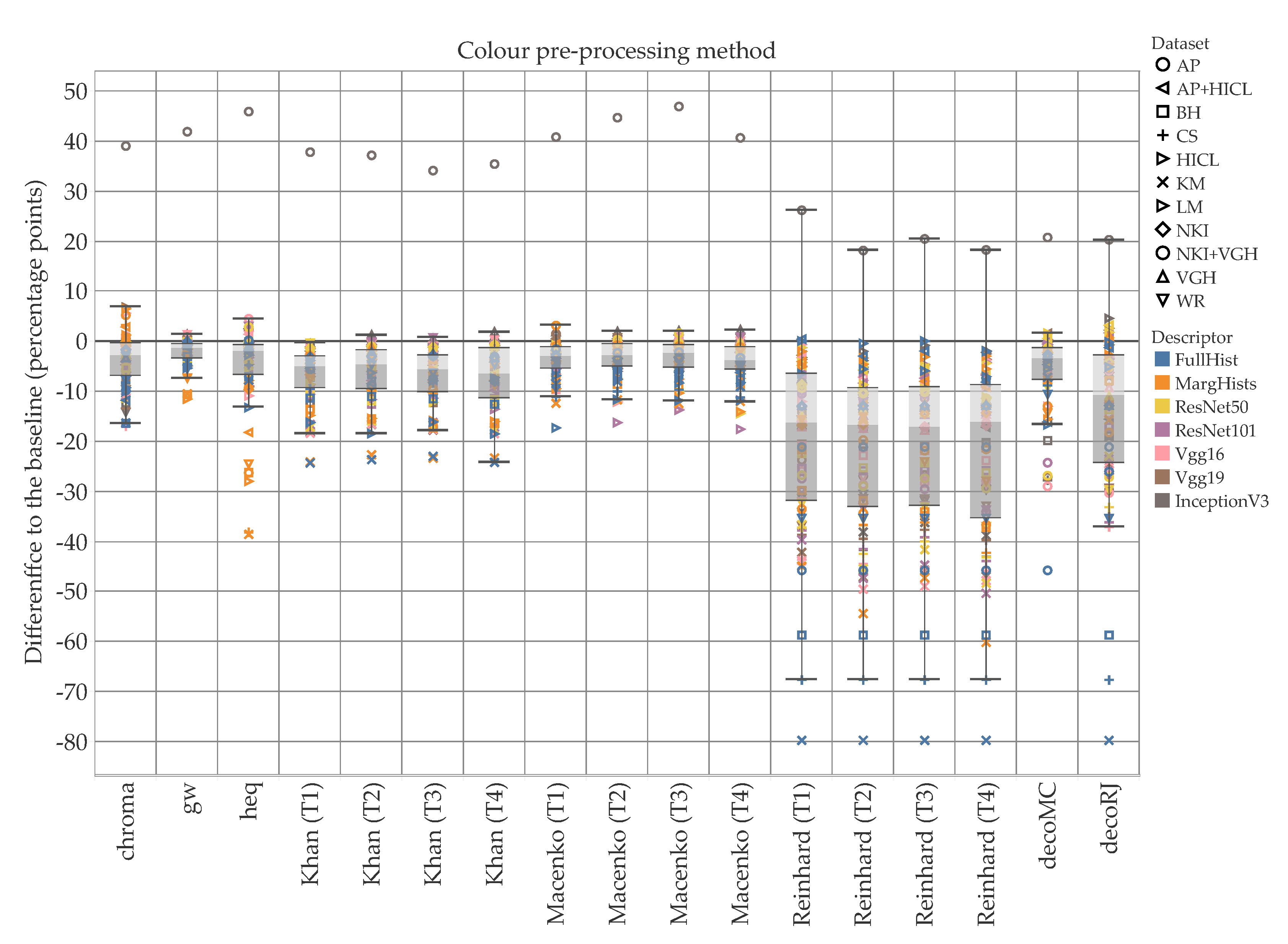
5.1. Accuracy
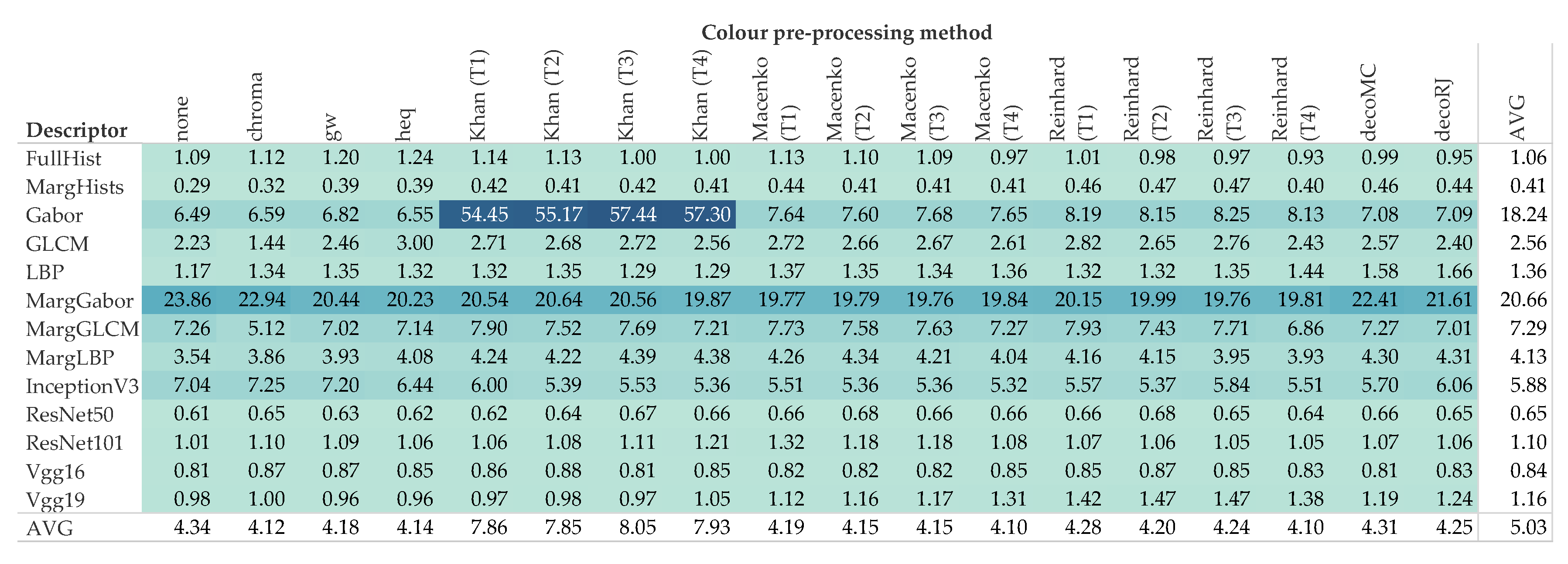
5.2. Computational Demand
6. Conclusions
Author Contributions
Funding
Acknowledgments
Conflicts of Interest
Abbreviations
| CNN | Convolutional Neural Network(s) |
| GLCM | Grey-level Co-occurrence Matrices |
| H&E | Hematoxilyn & Eosin |
| LBP | Local Binary Patterns |
| TCGA | The Cancer Genome Atlas |
| TMA | Tissue Micro-array(s) |
References
- Madabhushi, A. Digital pathology image analysis: Opportunities and challenges. Imaging Med. 2009, 1, 7–10. [Google Scholar] [CrossRef] [PubMed] [Green Version]
- Słodkowska, J.; García-Rojo, M. Digital pathology in personalized cancer therapy. Stud. Health Technol. Inform. 2012, 179, 143–154. [Google Scholar] [CrossRef] [PubMed] [Green Version]
- Siregar, P.; Julen, N.; Hufnagl, P.; Mutter, G.L. Computational morphogenesis—Embryogenesis, cancer research and digital pathology. Bio Syst. 2018, 169–170, 40–54. [Google Scholar] [CrossRef] [PubMed]
- Williams, B.J.; Lee, J.; Oien, K.A.; Treanor, D. Digital pathology access and usage in the UK: Results from a national survey on behalf of the National Cancer Research Institute’s CM-Path initiative. J. Clin. Pathol. 2018, 71, 463–466. [Google Scholar] [CrossRef]
- Parwani, A.V. Digital pathology enhances cancer diagnostics. MLO Med Lab. Obs. 2017, 49, 25. [Google Scholar]
- Kwak, J.T.; Hewitt, S.M. Multiview boosting digital pathology analysis of prostate cancer. Comput. Methods Programs Biomed. 2017, 142, 91–99. [Google Scholar] [CrossRef]
- Heindl, A.; Nawaz, S.; Yuan, Y. Mapping spatial heterogeneity in the tumor microenvironment: A new era for digital pathology. Lab. Investig. 2015, 95, 377–384. [Google Scholar] [CrossRef] [Green Version]
- Pell, R.; Oien, K.; Robinson, M.; Pitman, H.; Rajpoot, N.; Rittscher, J.; Snead, D.; Verrill, C.; UK National Cancer Research Institute (NCRI) Cellular-Molecular Pathology (CM-Path) Quality Assurance Working Group’s. The use of digital pathology and image analysis in clinical trials. J. Pathol. Clin. Res. 2019, 5, 81–90. [Google Scholar] [CrossRef] [Green Version]
- Bera, K.; Schalper, K.A.; Rimm, D.L.; Velcheti, V.; Madabhushi, A. Artificial intelligence in digital pathology—new tools for diagnosis and precision oncology. Nat. Rev. Clin. Oncol. 2019, 16, 703–715. [Google Scholar] [CrossRef]
- Griffin, J.; Treanor, D. Digital pathology in clinical use: Where are we now and what is holding us back? Histopathology 2017, 70, 134–145. [Google Scholar] [CrossRef]
- Lutsyk, M.; Ben-Izhak, O.; Sabo, E. Novel computerized method of pattern recognition of microscopic images in pathology for differentiating between malignant and benign lesions of the colon. Anal. Quant. Cytopathol. Histopathol. 2016, 38, 270–276. [Google Scholar]
- Sudharshan, P.; Petitjean, C.; Spanhol, F.; Oliveira, L.; Heutte, L.; Honeine, P. Multiple instance learning for histopathological breast cancer image classification. Expert Syst. Appl. 2019, 117, 103–111. [Google Scholar] [CrossRef]
- Yao, H.; Zhang, X.; Zhou, X.; Liu, S. Parallel structure deep neural network using CNN and RNN with an attention mechanism for breast cancer histology image classification. Cancers 2019, 11, 1901. [Google Scholar] [CrossRef] [PubMed] [Green Version]
- Yari, Y.; Nguyen, T.V.; Nguyen, H.T. Deep learning applied for histological diagnosis of breast cancer. IEEE Access 2020, 8, 162432–162448. [Google Scholar] [CrossRef]
- Sparks, R.; Madabhushi, A. Statistical shape model for manifold regularization: Gleason grading of prostate histology. Comput. Vis. Image Underst. 2013, 117, 1138–1146. [Google Scholar] [CrossRef] [Green Version]
- Dimitropoulos, K.; Barmpoutis, P.; Zioga, C.; Kamas, A.; Patsiaoura, K.; Grammalidis, N. Grading of invasive breast carcinoma through Grassmannian VLAD encoding. PLoS ONE 2017, 12, e0185110. [Google Scholar] [CrossRef] [Green Version]
- Jørgensen, A.; Emborg, J.; Røge, R.; Østergaard, L. Exploiting Multiple Color Representations to Improve Colon Cancer Detection in Whole Slide H&E Stains. In Proceedings of the 1st International Workshop on Computational Pathology (COMPAY), Granada, Spain, 16–20 September 2018; Volume 11039, pp. 61–68. [Google Scholar]
- Saxena, S.; Gyanchandani, M. Machine Learning Methods for Computer-Aided Breast Cancer Diagnosis Using Histopathology: A Narrative Review. J. Med. Imaging Radiat. Sci. 2020, 51, 182–193. [Google Scholar] [CrossRef]
- Martino, F.; Varricchio, S.; Russo, D.; Merolla, F.; Ilardi, G.; Mascolo, M.; dell’Aversana, G.; Califano, L.; Toscano, G.; De Pietro, G.; et al. A Machine-learning Approach for the Assessment of the Proliferative Compartment of Solid Tumors on Hematoxylin-Eosin-Stained Sections. Cancers 2020, 12, 1344. [Google Scholar] [CrossRef]
- Linder, N.; Konsti, J.; Turkki, R.; Rahtu, E.; Lundin, M.; Nordling, S.; Haglund, C.; Ahonen, T.; Pietikäinen, M.; Lundin, J. Identification of tumor epithelium and stroma in tissue microarrays using texture analysis. Diagn. Pathol. 2012, 7, 1–11. [Google Scholar] [CrossRef] [Green Version]
- Kather, J.; Weis, C.A.; Bianconi, F.; Melchers, S.; Schad, L.; Gaiser, T.; Marx, A.; Zöllner, F. Multi-class texture analysis in colorectal cancer histology. Sci. Rep. 2016, 6, 27988. [Google Scholar] [CrossRef]
- Khan, A.; Rajpoot, N.; Treanor, D.; Magee, D. A nonlinear mapping approach to stain normalization in digital histopathology images using image-specific color deconvolution. IEEE Trans. Biomed. Eng. 2014, 61, 1729–1738. [Google Scholar] [CrossRef] [PubMed]
- Komura, D.; Ishikawa, S. Machine Learning Methods for Histopathological Image Analysis. Comput. Struct. Biotechnol. J. 2018, 16, 34–42. [Google Scholar] [CrossRef] [PubMed]
- Clarke, E.L.; Treanor, D. Colour in digital pathology: A review. Histopathology 2017, 70, 153–163. [Google Scholar] [CrossRef] [PubMed] [Green Version]
- Macenko, M.; Niethammer, M.; Marron, J.; Borland, D.; Woosley, J.; Guan, X.; Schmitt, C.; Thomas, N. A method for normalizing histology slides for quantitative analysis. In Proceedings of the IEEE International Symposium on Biomedical Imaging: From Nano to Macro (ISBI), Boston, MA, USA, 28 June–1 July 2009; pp. 1107–1110. [Google Scholar]
- Ruifrok, A.; Johnston, D. Quantification of histochemical staining by color deconvolution. Anal. Quant. Cytol. Histol. 2001, 23, 291–299. [Google Scholar]
- Zanjani, F.G.; Zinger, S.; Bejnordi, B.E.; van der Laak, J.A.W.M.; de With, P.H.N. Stain normalization of histopathology images using generative adversarial networks. In Proceedings of the 2018 IEEE 15th International Symposium on Biomedical Imaging (ISBI 2018), Washington, DC, USA, 4–7 April 2018; pp. 573–577. [Google Scholar] [CrossRef]
- Shaban, M.T.; Baur, C.; Navab, N.; Albarqouni, S. Staingan: Stain Style Transfer for Digital Histological Images. In Proceedings of the 2019 IEEE 16th International Symposium on Biomedical Imaging (ISBI 2019), Venice, Italy, 8–11 April 2019; pp. 953–956. [Google Scholar] [CrossRef] [Green Version]
- Roy, S.; Kumar Jain, A.; Lal, S.; Kini, J. A study about color normalization methods for histopathology images. Micron 2018, 114, 42–61. [Google Scholar] [CrossRef]
- Li, X.; Plataniotis, K.N. Circular Mixture Modeling of Color Distribution for Blind Stain Separation in Pathology Images. IEEE J. Biomed. Health Inform. 2017, 21, 150–161. [Google Scholar] [CrossRef]
- Janowczyk, A.; Basavanhally, A.; Madabhushi, A. Stain Normalization using Sparse AutoEncoders (StaNoSA): Application to digital pathology. Comput. Med Imaging Graph. Off. J. Comput. Med Imaging Soc. 2017, 57, 50–61. [Google Scholar] [CrossRef] [Green Version]
- Sethi, A.; Sha, L.; Vahadane, A.; Deaton, R.; Kumar, N.; MacIas, V.; Gann, P. Empirical comparison of color normalization methods for epithelial-stromal classification in H and E images. J. Pathol. Inform. 2016, 7, 17. [Google Scholar] [CrossRef]
- Ciompi, F.; Geessink, O.; Bejnordi, B.E.; de Souza, G.S.; Baidoshvili, A.; Litjens, G.; van Ginneken, B.; Nagtegaal, I.; van der Laak, J. The importance of stain normalization in colorectal tissue classification with convolutional networks. In Proceedings of the IEEE International Symposium on Biomedical Imaging, Melbourne, Australia, 18–21 April 2017. [Google Scholar]
- Gadermayr, M.; Cooper, S.; Klinkhammer, B.; Boor, P.; Merhof, D. A quantitative assessment of image normalization for classifying histopathological tissue of the kidney. In Proceedings of the 39th German Conference on Pattern Recognition (GCPR), Basel, Switzerland, 12–15 September 2017; Volume 10496, pp. 3–13. [Google Scholar]
- Hameed, Z.; Zahia, S.; Garcia-Zapirain, B.; Aguirre, J.; Vanegas, A. Breast cancer histopathology image classification using an ensemble of deep learning models. Sensors 2020, 20, 4373. [Google Scholar] [CrossRef]
- Tellez, D.; Litjens, G.; Bándi, P.; Bulten, W.; Bokhorst, J.M.; Ciompi, F.; van der Laak, J. Quantifying the effects of data augmentation and stain color normalization in convolutional neural networks for computational pathology. Med Image Anal. 2019, 58, 101544. [Google Scholar] [CrossRef] [Green Version]
- Vahadane, A.; Peng, T.; Sethi, A.; Albarqouni, S.; Wang, L.; Baust, M.; Steiger, K.; Schlitter, A.M.; Esposito, I.; Navab, N. Structure-Preserving Color Normalization and Sparse Stain Separation for Histological Images. IEEE Trans. Med. Imaging 2016, 35, 1962–1971. [Google Scholar] [CrossRef] [PubMed]
- Bianconi, F.; Kather, J.; Reyes-Aldasoro, C. Evaluation of colour pre-processing on patch-based classification of H&E-stained images. In Proceedings of the 15th European Congress on Digital Pathology, ECDP 2019, Warwick, UK, 10–13 April 2019; Volume 11435, pp. 56–64. [Google Scholar]
- Spanhol, F.; Oliveira, L.; Petitjean, C.; Heutte, L. A Dataset for Breast Cancer Histopathological Image Classification. IEEE Trans. Biomed. Eng. 2016, 63, 1455–1462. [Google Scholar] [CrossRef] [PubMed]
- Gertych, A.; Ing, N.; Ma, Z.; Fuchs, T.; Salman, S.; Mohanty, S.; Bhele, S.; Velásquez-Vacca, A.; Amin, M.; Knudsen, B. Machine learning approaches to analyze histological images of tissues from radical prostatectomies. Comput. Med Imaging Graph. 2015, 46, 197–208. [Google Scholar] [CrossRef] [PubMed] [Green Version]
- Kostopoulos, S.; Glotsos, D.; Cavouras, D.; Daskalakis, A.; Kalatzis, I.; Georgiadis, P.; Bougioukos, P.; Ravazoula, P.; Nikiforidis, G. Computer-based association of the texture of expressed estrogen receptor nuclei with histologic grade using immunohistochemically-stained breast carcinomas. Anal. Quant. Cytol. Histol. 2009, 31, 187–196. [Google Scholar]
- Kather, J.N.; Zöllner, F.G.; Bianconi, F.; Melchers, S.M.; Schad, L.R.; Gaiser, T.; Marx, A.; Weis, C.A. Collection of Textures in Colorectal Cancer Histology. 2016. Version 1.0. Available online: https://zenodo.org/record/53169 (accessed on 6 November 2018).
- Shamir, L.; Orlov, N.; Mark Eckley, D.; Macura, T.; Goldberg, I. IICBU 2008: A proposed benchmark suite for biological image analysis. Med. Biol. Eng. Comput. 2008, 46, 943–947. [Google Scholar] [CrossRef] [Green Version]
- National Institute on Aging. Lymphoma. 2008. Available online: https://ome.grc.nia.nih.gov/iicbu2008/lymphoma/index.html (accessed on 6 November 2018).
- Beck, A.; Sangoi, A.; Leung, S.; Marinelli, R.; Nielsen, T.; Van De Vijver, M.; West, R.; Van De Rijn, M.; Koller, D. Imaging: Systematic analysis of breast cancer morphology uncovers stromal features associated with survival. Sci. Transl. Med. 2011, 3, 108ra113. [Google Scholar] [CrossRef] [Green Version]
- Beck, A.; Sangoi, A.; Leung, S.; Marinelli, R.; Nielsen, T.; Van De Vijver, M.; West, R.; Van De Rijn, M.; Koller, D. Systematic Analysis of Breast Cancer Morphology Uncovers Stromal Features Associated with Survival: Supplementary Documents. 2011. Available online: https://tma.im/tma_portal/C-Path/supp.html (accessed on 7 November 2018).
- Warwick-QU. 2015. Available online: https://warwick.ac.uk/fac/sci/dcs/research/tia/glascontest/download/ (accessed on 7 November 2018).
- Sirinukunwattana, K.; Snead, D.; Rajpoot, N. A Stochastic Polygons Model for Glandular Structures in Colon Histology Images. IEEE Trans. Med. Imaging 2015, 34, 2366–2378. [Google Scholar] [CrossRef] [Green Version]
- Sirinukunwattana, K.; Pluim, J.; Chen, H.; Qi, X.; Heng, P.A.; Guo, Y.; Wang, L.; Matuszewski, B.; Bruni, E.; Sanchez, U.; et al. Gland segmentation in colon histology images: The GlaS challenge contest. Med. Image Anal. 2017, 35, 489–502. [Google Scholar] [CrossRef] [Green Version]
- Kather, J.N.; Krisam, J.; Charoentong, P.; Luedde, T.; Herpel, E.; Weis, C.A.; Gaiser, T.; Marx, A.; Valous, N.A.; Ferber, D.; et al. Predicting survival from colorectal cancer histology slides using deep learning: A retrospective multicenter study. PLoS Med. 2019, 16, e1002730. [Google Scholar] [CrossRef]
- Skrede, O.J.; Raedt, S.D.; Kleppe, A.; Hveem, T.S.; Liestøl, K.; Maddison, J.; Askautrud, H.A.; Pradhan, M.; Nesheim, J.A.; Albregtsen, F.; et al. Deep learning for prediction of colorectal cancer outcome: A discovery and validation study. Lancet 2020, 395, 350–360. [Google Scholar] [CrossRef]
- Haub, P.; Meckel, T. A model based survey of colour deconvolution in diagnostic brightfield microscopy: Error estimation and spectral consideration. Sci. Rep. 2015, 5, 12096. [Google Scholar] [CrossRef] [PubMed]
- Stain Normalisation Toolbox. Available online: https://warwick.ac.uk/fac/sci/dcs/research/tia/software/sntoolbox/ (accessed on 8 November 2018).
- Foster, D. Color constancy. Vis. Res. 2011, 51, 674–700. [Google Scholar] [CrossRef] [PubMed]
- Cusano, C.; Napoletano, P.; Schettini, R. Evaluating color texture descriptors under large variations of controlled lighting conditions. J. Opt. Soc. Am. A Opt. Image Sci. Vis. 2016, 33, 17–30. [Google Scholar] [CrossRef] [PubMed] [Green Version]
- Reinhard, E.; Ashikhmin, M.; Gooch, B.; Shirley, P. Color transfer between images. IEEE Comput. Graph. Appl. 2001, 21, 34–41. [Google Scholar] [CrossRef]
- Cernadas, E.; Fernández-Delgado, M.; González-Rufino, E.; Carrión, P. Influence of normalization and color space to color texture classification. Pattern Recognit. 2017, 61, 120–138. [Google Scholar] [CrossRef]
- Finlayson, G.; Schaefer, G. Colour indexing across devices and viewing conditions. In Proceedings of the 2nd International Workshop on Content-Based Multimedia Indexing, Florence, Italy, 19–21 June 2017; pp. 215–221. [Google Scholar]
- van de Weijer, J. Color in Computer Vision. Available online: http://lear.inrialpes.fr/people/vandeweijer/research.html (accessed on 1 October 2019).
- Napoletano, P. Hand-Crafted vs Learned Descriptors for Color Texture Classification. In Proceedings of the 6th Computational Color Imaging Workshop (CCIW’17), Milan, Italy, 29–31 March 2017; Volume 10213, pp. 259–271. [Google Scholar]
- González, E.; Bianconi, F.; Álvarez, M.; Saetta, S. Automatic characterization of the visual appearance of industrial materials through colour and texture analysis: An overview of methods and applications. Adv. Opt. Technol. 2013, 2013, 503541. [Google Scholar] [CrossRef] [Green Version]
- Swain, M.; Ballard, D. Color indexing. Int. J. Comput. Vis. 1991, 7, 11–32. [Google Scholar] [CrossRef]
- Pietikainen, M.; Nieminen, S.; Marszalec, E.; Ojala, T. Accurate color discrimination with classification based on feature distributions. In Proceedings of the International Conference on Pattern Recognition (ICPR), Vienna, Austria, 25–29 August 1996; Volume 3, pp. 833–838. [Google Scholar]
- Haralick, R.M.; Shanmugam, K.; Dinstein, I. Textural Features for Image Classification. IEEE Trans. Syst. Man Cybern. 1973, 3, 610–621. [Google Scholar] [CrossRef] [Green Version]
- Bianconi, F.; Fernández, A. Rotation invariant co-occurrence features based on digital circles and discrete Fourier transform. Pattern Recognit. Lett. 2014, 48, 34–41. [Google Scholar] [CrossRef]
- Lahajnar, F.; Kovačič, S. Rotation-invariant texture classification. Pattern Recognit. Lett. 2003, 24, 706–719. [Google Scholar] [CrossRef]
- Ojala, T.; Pietikäinen, M.; Mäenpää, T. Multiresolution gray-scale and rotation invariant texture classification with local binary patterns. IEEE Trans. Pattern Anal. Mach. Intell. 2002, 24, 971–987. [Google Scholar] [CrossRef]
- Bianconi, F.; Bello-Cerezo, R.; Napoletano, P. Improved opponent color local binary patterns: An effective local image descriptor for color texture classification. J. Electron. Imaging 2018, 27, 011002. [Google Scholar] [CrossRef]
- Bello-Cerezo, R.; Bianconi, F.; Di Maria, F.; Napoletano, P.; Smeraldi, F. Comparative Evaluation of Hand-Crafted Image Descriptors vs. Off-the-Shelf CNN-Based Features for Colour Texture Classification under Ideal and Realistic Conditions. Appl. Sci. 2019, 9, 738. [Google Scholar] [CrossRef] [Green Version]
- Szegedy, C.; Vanhoucke, V.; Ioffe, S.; Shlens, J.; Wojna, Z. Rethinking the Inception Architecture for Computer Vision. In Proceedings of the IEEE Computer Society Conference on Computer Vision and Pattern Recognition, Las Vegas, NV, USA, 27–30 June 2016; pp. 2818–2826. [Google Scholar]
- He, K.; Zhang, X.; Ren, S.; Sun, J. Deep residual learning for image recognition. In Proceedings of the IEEE Computer Society Conference on Computer Vision and Pattern Recognition, Las Vegas, NV, USA, 27–30 June 2016; pp. 770–778. [Google Scholar]
- Chatfield, K.; Simonyan, K.; Vedaldi, A.; Zisserman, A. Return of the devil in the details: Delving deep into convolutional nets. In Proceedings of the British Machine Vision Conference, Nottingham, UK, 1–5 September 2014. [Google Scholar]
- Bianconi, F. CATAcOMB: Colour and Texture Analysis Toolbox for MatlaB. Available online: https://bitbucket.org/biancovic/catacomb/src/master/ (accessed on 21 September 2020).
- Vedaldi, A.; Lenc, K. MatConvNet: Convolutional neural networks for MATLAB. In Proceedings of the 23rd ACM International Conference on Multimedia (MM 2015), Brisbane, Australia, 26–30 October 2015; pp. 689–692. [Google Scholar]
- Shaban, M.; Khurram, S.A.; Fraz, M.M.; Alsubaie, N.; Masood, I.; Mushtaq, S.; Hassan, M.; Loya, A.; Rajpoot, N.M. A Novel Digital Score for Abundance of Tumour Infiltrating Lymphocytes Predicts Disease Free Survival in Oral Squamous Cell Carcinoma. Sci. Rep. 2019, 9, 13341. [Google Scholar] [CrossRef] [Green Version]
- Mobadersany, P.; Yousefi, S.; Amgad, M.; Gutman, D.A.; Barnholtz-Sloan, J.S.; Vega, J.E.V.; Brat, D.J.; Cooper, L.A.D. Predicting cancer outcomes from histology and genomics using convolutional networks. Proc. Natl. Acad. Sci. USA 2018, 115, E2970–E2979. [Google Scholar] [CrossRef] [PubMed] [Green Version]
- Bychkov, D.; Linder, N.; Turkki, R.; Nordling, S.; Kovanen, P.E.; Verrill, C.; Walliander, M.; Lundin, M.; Haglund, C.; Lundin, J. Deep learning based tissue analysis predicts outcome in colorectal cancer. Sci. Rep. 2018, 8, 3395. [Google Scholar] [CrossRef]
- Jiang, D.; Liao, J.; Duan, H.; Wu, Q.; Owen, G.; Shu, C.; Chen, L.; He, Y.; Wu, Z.; He, D.; et al. A machine learning-based prognostic predictor for stage III colon cancer. Sci. Rep. 2020, 10, 10333. [Google Scholar] [CrossRef]


| Model | Ref. | Layer (Name/No.) | No. of Features |
|---|---|---|---|
| InceptionV3 | [70] | 313 | 2048 |
| ResNet50 | [71] | ‘pool5’ | 2048 |
| ResNet101 | [71] | ‘pool5’ | 2048 |
| Vgg16 | [72] | ‘FC-4096’ | 4096 |
| Vgg19 | [72] | ‘FC-4096’ | 4096 |
| Dataset | Rank | Accuracy (%) | Descriptor | Pre-Processing |
|---|---|---|---|---|
| AP | 1 | 81.79 | MargGLCM | decoMC |
| 2 | 81.70 | FullHist | heq | |
| AP+HICL | 1 | 68.97 | ResNet50 | decoRJ |
| 2 | 67.61 | FullHist | Reinhard (T1) | |
| BH | 1 | 90.67 | ResNet101 | none |
| 2 | 90.07 | ResNet50 | none | |
| CS | 1 | 87.59 | FullHist | none |
| 2 | 86.39 | ResNet50 | none | |
| HICL | 1 | 51.58 | ResNet101 | decoMC |
| 2 | 51.51 | InceptionV3 | decoRJ | |
| KM | 1 | 92.18 | FullHist | none |
| 2 | 89.03 | MargHists | chroma | |
| Lymphoma | 1 | 85.98 | MargHists | chroma |
| 2 | 84.53 | FullHist | none | |
| NKI | 1 | 98.87 | ResNet50 | none |
| 2 | 98.86 | ResNet50 | chroma | |
| NKI+VGH | 1 | 98.39 | ResNet50 | none |
| 2 | 98.33 | ResNet101 | gw | |
| VGH | 1 | 96.10 | ResNet101 | none |
| 2 | 96.00 | MargHists | decoRJ | |
| WR | 1 | 94.37 | ResNet50 | none |
| 2 | 94.11 | ResNet50 | Khan (CC140) |
Publisher’s Note: MDPI stays neutral with regard to jurisdictional claims in published maps and institutional affiliations. |
© 2020 by the authors. Licensee MDPI, Basel, Switzerland. This article is an open access article distributed under the terms and conditions of the Creative Commons Attribution (CC BY) license (http://creativecommons.org/licenses/by/4.0/).
Share and Cite
Bianconi, F.; Kather, J.N.; Reyes-Aldasoro, C.C. Experimental Assessment of Color Deconvolution and Color Normalization for Automated Classification of Histology Images Stained with Hematoxylin and Eosin. Cancers 2020, 12, 3337. https://doi.org/10.3390/cancers12113337
Bianconi F, Kather JN, Reyes-Aldasoro CC. Experimental Assessment of Color Deconvolution and Color Normalization for Automated Classification of Histology Images Stained with Hematoxylin and Eosin. Cancers. 2020; 12(11):3337. https://doi.org/10.3390/cancers12113337
Chicago/Turabian StyleBianconi, Francesco, Jakob N. Kather, and Constantino Carlos Reyes-Aldasoro. 2020. "Experimental Assessment of Color Deconvolution and Color Normalization for Automated Classification of Histology Images Stained with Hematoxylin and Eosin" Cancers 12, no. 11: 3337. https://doi.org/10.3390/cancers12113337