A Choice Prediction Competition for Market Entry Games: An Introduction

Abstract

A choice prediction competition is organized that focuses on decisions from experience in market entry games (http://sites.google.com/site/gpredcomp/ and https://www.mdpi.com/si/games/predict-behavior/). The competition is based on two experiments: An estimation experiment, and a competition experiment. The two experiments use the same methods and subject pool, and examine games randomly selected from the same distribution. The current introductory paper presents the results of the estimation experiment, and clarifies the descriptive value of several baseline models. The experimental results reveal the robustness of eight behavioral tendencies that were documented in previous studies of market entry games and individual decisions from experience. The best baseline model (I-SAW) assumes reliance on small samples of experiences, and strong inertia when the recent results are not surprising. The competition experiment will be run in May 2010 (after the completion of this introduction), but they will not be revealed until September. To participate in the competition, researchers are asked to E-mail the organizers models (implemented in computer programs) that read the incentive structure as input, and derive the predicted behavior as an output. The submitted models will be ranked based on their prediction error. The winners of the competition will be invited to publish a paper that describes their model.

1. Background

Previous study of the effect of experience on economic behavior highlights the potential of simple learning models. Several investigations demonstrate that simple models can provide surprisingly accurate ex-ante predictions of behavior in some situations. For example, Erev and Roth [1] demonstrate that a 3-parameter reinforcement learning model provides useful predictions of choice rates in 12 games with unique mixed strategy equilibrium. Additional indications of the potential of simple learning models come from the observed similarities of the basic reaction to feedback across species (e.g., [2,3,4]), and the discovery that the activity of certain dopamine neurons is correlated with one of the terms assumed by reinforcement learning models [5].

However, more recent studies reveal that the task of advancing beyond the demonstrations of the potential of simple models is not simple. Different studies appear to support different models, and the relationship between the distinct results is not always clear [6].

We believe there are two main reasons for the inconsistencies in the learning-in-games literature. First is the fact that learning is only one of the factors that affect behavior in repeated games. Other important factors include: framing, fairness, reciprocation, and reputation. It is possible that different studies reached different conclusions because they studied learning in environments in which these important factors have different implications.

A second cause of confusion is a tendency to focus on relatively small data sets and relatively small sets of models. Erev and Roth [1] tried to address this problem by studying 12 games and two families of models. We now understand that this data set and group of models were not large enough. Recent research show that is surprisingly easy to over-fit learning data sets [7,8].

Erev et al. [9] took two measures to address these problems. The first is an extensive experimental study of the effect of experience under conditions that minimize the effect of other factors. The second is the organization of an open choice prediction competition that facilitates the evaluation of a wide class of models. Specifically, Erev et al. organized a simplified version of the competition run by Arifovic, McKelvey, and Pevnitskaya [10]. They ran two large experiments examining different problems drawn randomly from the same space, and challenged other researchers to predict the results of the second study based on evaluation of the results of the first study. The main result of (the repeated decisions from experience part of) that investigation was an indication of a clear advantage of models that assume instance-based reasoning (and reliance on small set of experiences) over more popular models that assume sequential adaptation of propensities (like reinforcement learning and fictitious play). The winner of the competition was an instance based model that assumes an ACT-R cognitive architecture (submitted by Stewart, West and Lebiere based on [11]).

The main goal of the current research is to extend Erev et al.’s competition along two dimensions. The first extension involves the source of uncertainty. Erev et al. focused on individual decisions under uncertainty; thus, the environment (state of nature) was the sole source of uncertainty in the situations they studied. The current study focuses on games that involve both environmental and strategic uncertainty. The second extension is related to the available feedback. Erev et al. focused on situations in which the feedback is limited to the obtained outcomes. The current study focuses on learning under more complete feedback.

We believe that the set of situations considered here (decisions under environmental and strategic uncertainty based on complete feedback when the role of framing, fairness, reciprocation and reputation is small) is more than a good test bed for learning models. This set of situations is also a simulation of many natural environments that have similar characteristics. One set of natural examples involve transportation dilemmas. When deciding how to commute to work, for example, commuters are likely to rely on past experience and pay limited attention to fairness and similar considerations. To clarify the relationship of the current investigation to this class of natural problems we chose to focus on Market Entry games [12,13,14] that model simple transportation dilemmas. Specifically, we consider 4-person 2-alternative Market Entry games. Each player in these games has to decide between a safe option and risky entry to a market in which the payoff decreases with the number of entrants. Under one transportation cover story the safer option abstracts “taking the train”, and the risky option abstracts “driving”.

Previous experimental studies of behavior in Market Entry games [14,15,16] reveal surprisingly fast convergence to Nash equilibrium. For example, experimental study of the market entry game presented in Table 1 documents convergence to equilibrium after 5 trials even when the players did not receive a description of the incentive structure [16]. At first glance this observation appears to be inconsistent with the observation of a robust deviation from maximization even after hundreds of trials in studies of individual decisions under uncertainty based on feedback [17]. However, it is possible that the same learning process leads to different behaviors in different environments (as in e.g. [18]). We hope that the present study will shed light on this possibility.

Table 1. An example of an experimental study of decisions from experience in a market entry game [16].

At each trial, each of 12 players has to decide (individually) between “entering a risky market”, or “staying out” (a safer prospect). The payoff from entering decreases with the number of entrants (E). The exact payoff for player i is at trial t is: $$V_i(t)=\{\begin{array}{cc}1+2(8\text{-E})& \text{if i enters}\\ 1& \text{if i does not enter}\end{array}$$ The participants did not receive a description of the incentive structure. Their information was limited to the payoff they received after each trial.

Table 1. An example of an experimental study of decisions from experience in a market entry game [16].

At each trial, each of 12 players has to decide (individually) between “entering a risky market”, or “staying out” (a safer prospect). The payoff from entering decreases with the number of entrants (E). The exact payoff for player i is at trial t is: $$V_i(t)=\{\begin{array}{cc}1+2(8\text{-E})& \text{if i enters}\\ 1& \text{if i does not enter}\end{array}$$ The participants did not receive a description of the incentive structure. Their information was limited to the payoff they received after each trial.

Like Erev et al.’s [9] competition, the current competition is based on the data from two lab experiments: an estimation experiment, and a competition experiment. The estimation experiment was run in March 2010 and focused on the 40 games presented in Table 2. The experimental procedure and the results obtained in this study are presented below. The competition experiment will be run after 28 April 2010 (after the completion of the current introduction paper). It will use the same method as the estimation experiment, but will focus on different games and different experimental subjects.

Table 2. The 40 market entry games that were studied in the estimation experiment. At each trial, each of four players has to decide (individually) between “entering a risky market”, or “staying out” (a safer prospect). The payoffs depend on a realization of a binary gamble (the realization at trial t is denoted G_t, and yields “H with probability Ph; and L otherwise”), the number of entrants (E), and two additional parameters (k and S). The exact payoff for player i at trial t is:

$$V_i(t)=\{\begin{array}{cc}10\text{-k}(\text{E})+{\text{G}}_{\text{t}}& \text{if i enters}\\ {\text{round}(\text{G}}_{\text{t}}/\text{S})\text{ with p}={\text{.5; -round}(\text{G}}_{\text{t}}/\text{S})\text{ otherwise}& \text{if i does not enter}\end{array}$$

The left hand-columns present the exact value of the different parameters in the 40 games, the right hand columns present the equilibrium predictions, and the main experimental results in the first and second block of 25 trials (B1 and B2).

								Experimental results
The games						Entry at eq.		Entry rates		Efficiency		Alternations
#	K	ph	H	L	S	pure	sym-metric	B1	B2	B1	B2	B1	B2
1	2	0.04	70	-3	5	1.00	1.00	0.71	0.80	2.77	2.66	0.18	0.15
2	2	0.23	30	-9	4	1.00	1.00	0.55	0.62	2.64	2.75	0.27	0.24
3	2	0.67	1	-2	3	1.00	1.00	0.88	0.94	2.39	2.24	0.12	0.04
4	2	0.73	30	-80	4	1.00	1.00	0.71	0.64	2.58	2.57	0.30	0.28
5	2	0.80	20	-80	5	1.00	1.00	0.66	0.67	2.50	2.67	0.34	0.28
6	2	0.83	4	-20	3	1.00	1.00	0.73	0.82	2.45	2.50	0.28	0.18
7	2	0.94	6	-90	5	1.00	1.00	0.86	0.87	2.34	2.38	0.15	0.13
8	2	0.95	1	-20	5	1.00	1.00	0.86	0.91	2.48	2.31	0.14	0.10
9	2	0.96	4	-90	3	1.00	1.00	0.87	0.90	2.36	2.34	0.14	0.08
10	3	0.10	70	-8	4	0.75	0.77	0.42	0.48	1.22	1.11	0.35	0.28
11	3	0.90	9	-80	4	0.75	0.77	0.80	0.73	-0.33	0.29	0.20	0.24
12	3	0.91	7	-70	6	0.75	0.77	0.76	0.83	0.10	-0.41	0.21	0.14
13	4	0.06	60	-4	2	0.50	0.50	0.42	0.41	0.52	0.84	0.27	0.17
14	4	0.20	40	-10	4	0.50	0.50	0.48	0.46	-0.34	0.04	0.36	0.34
15	4	0.31	20	-9	4	0.50	0.50	0.49	0.44	-0.07	0.30	0.38	0.37
16	4	0.60	4	-6	2	0.50	0.50	0.56	0.58	-0.27	-0.26	0.28	0.30
17	4	0.60	40	-60	3	0.50	0.50	0.58	0.55	-0.96	-0.20	0.33	0.28
18	4	0.73	3	-8	2	0.50	0.50	0.57	0.55	-0.29	0.09	0.26	0.23
19	4	0.80	20	-80	2	0.50	0.50	0.64	0.63	-1.30	-1.21	0.29	0.28
20	4	0.90	1	-9	6	0.50	0.50	0.53	0.48	0.12	0.63	0.24	0.18
21	4	0.96	3	-70	3	0.50	0.50	0.65	0.62	-0.84	-0.38	0.27	0.19
22	5	0.02	80	-2	3	0.25	0.33	0.36	0.31	0.24	0.64	0.21	0.19
23	5	0.07	90	-7	3	0.25	0.33	0.39	0.24	-0.81	0.34	0.24	0.17
24	5	0.53	80	-90	5	0.25	0.33	0.65	0.58	-3.41	-2.44	0.29	0.38
25	5	0.80	1	-4	2	0.25	0.33	0.45	0.42	-0.31	0.11	0.24	0.19
26	5	0.88	4	-30	3	0.25	0.33	0.52	0.49	-0.95	-0.57	0.24	0.21
27	5	0.93	5	-70	4	0.25	0.33	0.57	0.57	-1.63	-1.43	0.31	0.24
28	6	0.10	90	-10	5	0.25	0.22	0.26	0.27	-0.13	0.07	0.25	0.20
29	6	0.19	30	-7	3	0.25	0.22	0.39	0.32	-1.35	-0.45	0.29	0.28
30	6	0.29	50	-20	3	0.25	0.22	0.47	0.48	-2.74	-2.43	0.40	0.36
31	6	0.46	7	-6	6	0.25	0.22	0.38	0.34	-0.90	-0.38	0.27	0.24
32	6	0.57	6	-8	4	0.25	0.22	0.44	0.39	-1.56	-0.59	0.28	0.29
33	6	0.82	20	-90	3	0.25	0.22	0.63	0.55	-5.33	-3.14	0.32	0.24
34	6	0.88	8	-60	4	0.25	0.22	0.57	0.50	-3.30	-1.96	0.22	0.22
35	7	0.06	90	-6	4	0.25	0.14	0.31	0.35	-1.40	-1.43	0.31	0.24
36	7	0.21	30	-8	3	0.25	0.14	0.39	0.31	-2.20	-1.04	0.35	0.26
37	7	0.50	80	-80	5	0.25	0.14	0.51	0.55	-4.18	-4.78	0.37	0.40
38	7	0.69	9	-20	5	0.25	0.14	0.46	0.34	-2.62	-0.88	0.31	0.23
39	7	0.81	7	-30	2	0.25	0.14	0.41	0.34	-2.25	-0.93	0.27	0.25
40	7	0.91	1	-10	2	0.25	0.14	0.34	0.27	-0.71	-0.30	0.22	0.20
Means Estimated error variance						0.51	0.51	0.56 .0016	0.54 .0015	-.0.39 .1370	0.04 .1188	0.27 .0018	0.23 .0015

Table 2. The 40 market entry games that were studied in the estimation experiment. At each trial, each of four players has to decide (individually) between “entering a risky market”, or “staying out” (a safer prospect). The payoffs depend on a realization of a binary gamble (the realization at trial t is denoted G_t, and yields “H with probability Ph; and L otherwise”), the number of entrants (E), and two additional parameters (k and S). The exact payoff for player i at trial t is:

$$V_i(t)=\{\begin{array}{cc}10\text{-k}(\text{E})+{\text{G}}_{\text{t}}& \text{if i enters}\\ {\text{round}(\text{G}}_{\text{t}}/\text{S})\text{ with p}={\text{.5; -round}(\text{G}}_{\text{t}}/\text{S})\text{ otherwise}& \text{if i does not enter}\end{array}$$

The left hand-columns present the exact value of the different parameters in the 40 games, the right hand columns present the equilibrium predictions, and the main experimental results in the first and second block of 25 trials (B1 and B2).

								Experimental results
The games						Entry at eq.		Entry rates		Efficiency		Alternations
#	K	ph	H	L	S	pure	sym-metric	B1	B2	B1	B2	B1	B2
1	2	0.04	70	-3	5	1.00	1.00	0.71	0.80	2.77	2.66	0.18	0.15
2	2	0.23	30	-9	4	1.00	1.00	0.55	0.62	2.64	2.75	0.27	0.24
3	2	0.67	1	-2	3	1.00	1.00	0.88	0.94	2.39	2.24	0.12	0.04
4	2	0.73	30	-80	4	1.00	1.00	0.71	0.64	2.58	2.57	0.30	0.28
5	2	0.80	20	-80	5	1.00	1.00	0.66	0.67	2.50	2.67	0.34	0.28
6	2	0.83	4	-20	3	1.00	1.00	0.73	0.82	2.45	2.50	0.28	0.18
7	2	0.94	6	-90	5	1.00	1.00	0.86	0.87	2.34	2.38	0.15	0.13
8	2	0.95	1	-20	5	1.00	1.00	0.86	0.91	2.48	2.31	0.14	0.10
9	2	0.96	4	-90	3	1.00	1.00	0.87	0.90	2.36	2.34	0.14	0.08
10	3	0.10	70	-8	4	0.75	0.77	0.42	0.48	1.22	1.11	0.35	0.28
11	3	0.90	9	-80	4	0.75	0.77	0.80	0.73	-0.33	0.29	0.20	0.24
12	3	0.91	7	-70	6	0.75	0.77	0.76	0.83	0.10	-0.41	0.21	0.14
13	4	0.06	60	-4	2	0.50	0.50	0.42	0.41	0.52	0.84	0.27	0.17
14	4	0.20	40	-10	4	0.50	0.50	0.48	0.46	-0.34	0.04	0.36	0.34
15	4	0.31	20	-9	4	0.50	0.50	0.49	0.44	-0.07	0.30	0.38	0.37
16	4	0.60	4	-6	2	0.50	0.50	0.56	0.58	-0.27	-0.26	0.28	0.30
17	4	0.60	40	-60	3	0.50	0.50	0.58	0.55	-0.96	-0.20	0.33	0.28
18	4	0.73	3	-8	2	0.50	0.50	0.57	0.55	-0.29	0.09	0.26	0.23
19	4	0.80	20	-80	2	0.50	0.50	0.64	0.63	-1.30	-1.21	0.29	0.28
20	4	0.90	1	-9	6	0.50	0.50	0.53	0.48	0.12	0.63	0.24	0.18
21	4	0.96	3	-70	3	0.50	0.50	0.65	0.62	-0.84	-0.38	0.27	0.19
22	5	0.02	80	-2	3	0.25	0.33	0.36	0.31	0.24	0.64	0.21	0.19
23	5	0.07	90	-7	3	0.25	0.33	0.39	0.24	-0.81	0.34	0.24	0.17
24	5	0.53	80	-90	5	0.25	0.33	0.65	0.58	-3.41	-2.44	0.29	0.38
25	5	0.80	1	-4	2	0.25	0.33	0.45	0.42	-0.31	0.11	0.24	0.19
26	5	0.88	4	-30	3	0.25	0.33	0.52	0.49	-0.95	-0.57	0.24	0.21
27	5	0.93	5	-70	4	0.25	0.33	0.57	0.57	-1.63	-1.43	0.31	0.24
28	6	0.10	90	-10	5	0.25	0.22	0.26	0.27	-0.13	0.07	0.25	0.20
29	6	0.19	30	-7	3	0.25	0.22	0.39	0.32	-1.35	-0.45	0.29	0.28
30	6	0.29	50	-20	3	0.25	0.22	0.47	0.48	-2.74	-2.43	0.40	0.36
31	6	0.46	7	-6	6	0.25	0.22	0.38	0.34	-0.90	-0.38	0.27	0.24
32	6	0.57	6	-8	4	0.25	0.22	0.44	0.39	-1.56	-0.59	0.28	0.29
33	6	0.82	20	-90	3	0.25	0.22	0.63	0.55	-5.33	-3.14	0.32	0.24
34	6	0.88	8	-60	4	0.25	0.22	0.57	0.50	-3.30	-1.96	0.22	0.22
35	7	0.06	90	-6	4	0.25	0.14	0.31	0.35	-1.40	-1.43	0.31	0.24
36	7	0.21	30	-8	3	0.25	0.14	0.39	0.31	-2.20	-1.04	0.35	0.26
37	7	0.50	80	-80	5	0.25	0.14	0.51	0.55	-4.18	-4.78	0.37	0.40
38	7	0.69	9	-20	5	0.25	0.14	0.46	0.34	-2.62	-0.88	0.31	0.23
39	7	0.81	7	-30	2	0.25	0.14	0.41	0.34	-2.25	-0.93	0.27	0.25
40	7	0.91	1	-10	2	0.25	0.14	0.34	0.27	-0.71	-0.30	0.22	0.20
Means Estimated error variance						0.51	0.51	0.56 .0016	0.54 .0015	-.0.39 .1370	0.04 .1188	0.27 .0018	0.23 .0015

On 24 April 2010 (before running the competition experiment) we posted the data of the estimation experiment and a description of the baseline models (presented below) on the Web (http://sites.google.com/site/gpredcomp/ and https://www.mdpi.com/si/games/predict-behavior/; see also Web Appendices) and we are now inviting other researchers to participate in a competition that focuses on the prediction of the data of the second (competition) experiment. The call to participate in the competition will be published in the journal Games and in the e-mail lists of the leading scientific organizations that focus on decision-making, game theory, and behavioral economics. The competition is open to all; there are no prior requirements. The predictions submission deadline is 1 September 2010 (at midnight EST).

Researchers participating in the competition are allowed to study the results of the estimation study. Their goal is to develop a model that would predict the results of the competition study. The model has to be implemented in a computer program that reads the payoff distributions of the relevant games as an input and predicts the main results as output.

The parameters of the games, and their selection algorithm.

At each trial of the games studied here, each of four players has to decide (individually) between “entering a risky market”, or “staying out” (a safer prospect). The payoffs depend on a realization of a binary gamble (the realization at trial t is denoted G_t, and yields “H with probability Ph; and L otherwise”), the number of entrants (E), and two additional parameters (k and S). The exact payoff for player i at trial t is:

$$V_i(t)=\{\begin{array}{cc}10\text{-k}(\text{E})+{\text{G}}_{\text{t}}& \text{if i enters}\\ {\text{round}(\text{G}}_{\text{t}}/\text{S})\text{ with p}={\text{.5; -round}(\text{G}}_{\text{t}}/\text{S})\text{ otherwise}& \text{if i does not enter}\end{array}$$

(1)

The left-hand columns of Table 2 present the exact value of the different parameters of the 40 games that were studied in the estimation experiment. The problems were determined with a random selection of the parameters (k, S, L, M, H and Ph) using the algorithm described in Appendix 1. Notice that the algorithm implies that the expected value of the gamble is 0, and a uniform distribution of k between 2 and 7. These constraints imply that the risk neutral Nash equilibria of the games are determined by the value of k, and that the mean entry rate at equilibrium over games is 50% (these predictions are discussed in Section 5.1. below).

2. Experimental Method

The estimation experiment was run in March 2010 in the CLER lab at Harvard. One hundred and twenty students, members of the lab’s subject-pool that includes more than 2000 students, participated in the study. The study was run in eight independent sessions, each of which included between 12 and 20 participants. Each session focused on 10 of the 40 entry games presented in Table 2, and each subset of 10 games was run twice, counterbalancing the order of problems. The experiment was computerized using Z-tree [19]. After the instructions were read by the experimenter, each participant was randomly matched with three other participants and the four subjects then played each of the 10 games for 50 trials.

The participants’ payoff in each trial was computed by the game’s payoff rule described above. This rule implies that the payoff is a function of the player’s own choice, the choices of the other three participants in the group (such that the more people enter the less is the payoff from entry), and the trial’s state of nature. Participants did not receive a description of the payoff structure but received feedback after each trial, which included the result of their choice, and the result that they could receive had they selected otherwise (the “foregone” payoff).1 Notice that the incentive structure implies that the obtained payoff of the entrants (10-k(E) + G_t), is larger than the forgone payoff from entering observed by the players who did not enter (10-k(E+1) + G_t).

The whole procedure took about 70 minutes on average. Participants’ final payoffs were composed from the sum of a $25 show-up fee, their payoff (gain/loss) in one randomly selected trial, and a small bonus they received each time they responded within 4 seconds in a given trial. Final payoffs ranged between $18 and $36.25.

3. Experimental results

The “Entry rates,” “Efficiency,” and “Alternations” columns in Table 2 present the main results in the first block (B1, the first 25 trials) and the second block (B2, last 25 trials) in each game. The entry rates over games are higher than 50%, and are relatively stable over blocks. The difference between the first block (56%) and the second block (54%) is only marginally significant (t(39) = 1.87, p < .1 using game as a unit of analysis). Additional analysis reveals a higher entry rate in the very first trial (66%). This rate is significantly higher than 50% (t(119) = 6.36, p< .001 using participant as a unit of analysis). The observed entry rate in the very first trial (first trial in the first game played by each participant) is even higher (72%).

The efficiency columns present the observed expected payoffs. The expected payoff of Player i is 10-k(E) if i entered, and 0 otherwise. These columns show an increase in efficiency from -.39 in the first block, to +0.04 in the second block. The increase is significant (t(39) = 4.66, p < .0001).

The alternation columns present the proportion of times that players change their choices between trials (i.e., each trial in which a player chooses a different option than what she had chosen in the previous trial is marked as a “change”). The difference between the first block (27%) and the second block (23%) is small but highly significant (t(39) = 5.8, p < .0001).

Additional analyses reveal replications of eight behavioral regularities that have been observed in previous studies of market entry games and individual decisions from experience. These regularities are summarized below:

The payoff variability effect. Comparison of the observed entry rates in the second block with the equilibrium predictions reveals high correlations: 0.81, and 0.84 with the symmetric and pure strategy predictions respectively. The accuracy of the equilibrium predictions is particularly high in games with relatively low environmental uncertainty. For example, in Games 16 and 18 (absolute value of H and L below 10) the equilibrium predictions are 50% and the observed entry rates in both blocks are between 50% and 60%. This pattern is a replication of the results documented by Rapoport and his co-authors [14,15,16]. The bias of the equilibrium predictions increases with the standard deviation of the gamble. For example, the correlation between the “bias of the symmetric equilibrium prediction of the entry rate” and the standard deviation of the gamble is 0.47. This pattern is consistent with “the payoff variability effect” [20,21]: High payoff variability appears to reduce sensitivity to the incentive structure.

High sensitivity to forgone payoffs. Comparison of the effect of obtained and forgone payoffs reveals “high sensitivity to forgone payoffs”. For example, the tendency to repeat the last choice was slightly better predicted by the most recent forgone payoff than by the most recent obtained payoff. The absolute correlations between the probability of repetition (1 for repetition, 0 otherwise) and the recent payoffs (over all choices in trials 2 to 50) were 0.06 and 0.05 for the forgone and the obtained payoff respectively. Similar results are reported by Grosskopf et al. [22].

Excess entry. The proportion of choices of the risky alternative does not appear to reflect risk aversion and/or loss aversion [23]. The overall R-rate (55%) is higher than the predicted R-rate at equilibrium under the assumption of risk neutrality (less than 51%). Thus, the results reflect excess entry (see [24])

Underweighting of rare events. Analysis of the correlation between the parameters of the environmental uncertainty (H, Ph, and L) and the observed entry rates reveals an interesting pattern. The entry rates (using game as a unit of analysis) are positively correlated with Ph (0.54) and negatively correlated with H and L (-.40 and -.52). Recall that in the current set of games, Ph is negatively correlated with H and L (-.80 and -.59). Thus, the negative correlation of the entry rates with L and H can be a product of higher sensitivity to the probabilities than to the exact outcomes. This pattern is consistent with the observation of underweighting of rare events in decisions from experience (see [25]).

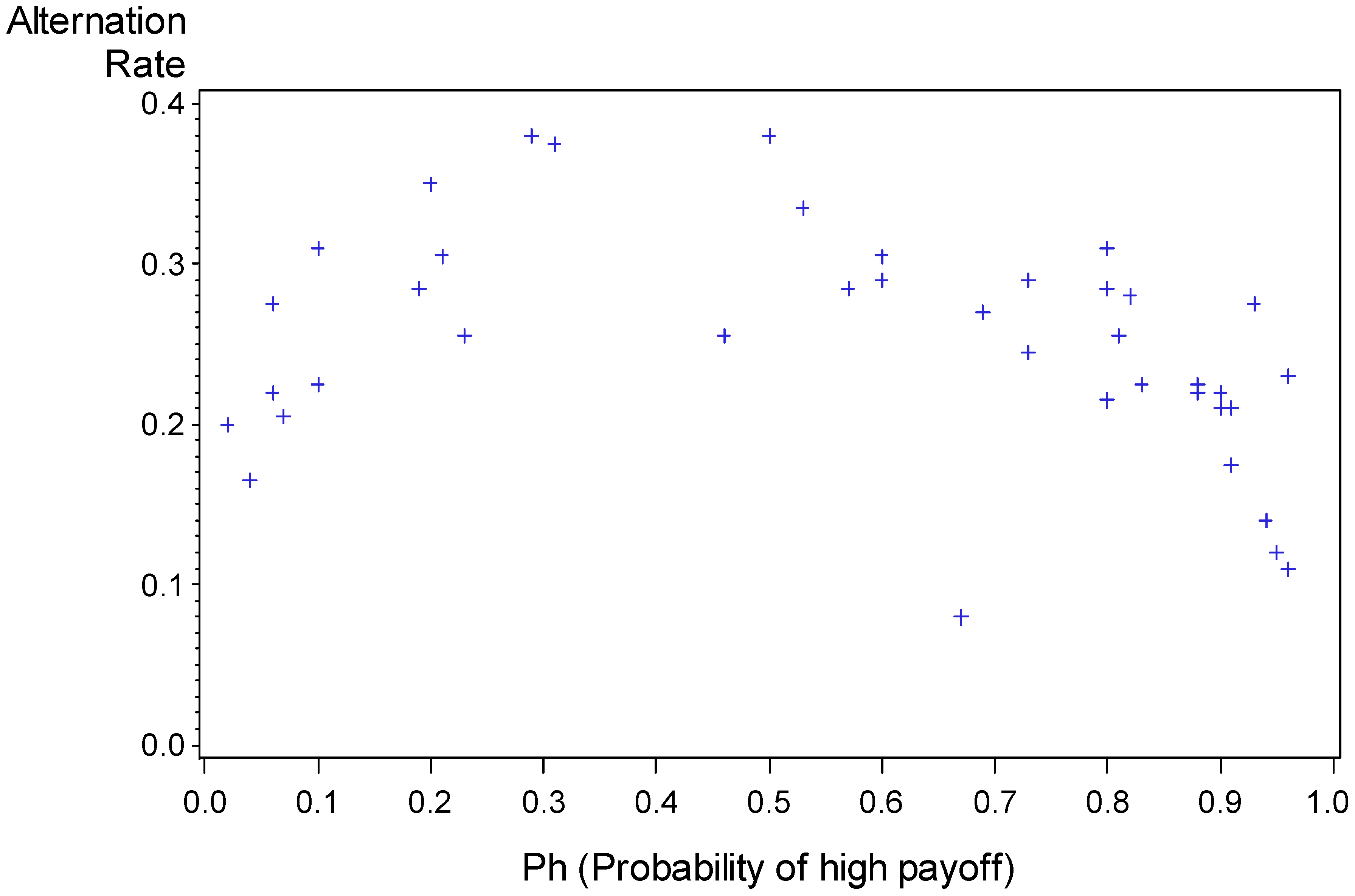
Surprise-triggers-change. Figure 1 presents the alternation rate as a function of Ph (using game as a unit of analysis). It reveals a reversed U relationship: The alternation rate is maximal when Ph is close to 0.5. Nevo and Erev [26] who observed a similar pattern in individual choice tasks note that it can be captured with the assertion that surprise-triggers-change.

Figure 1. Proportion of alternation as a function of Ph. Each data point summarizes the results of one game. The outlier (alternation rate of 0.08 when Ph = 0.67) is Problem 3 which involves the lowest payoff variance, and it is the only problem in which entry cannot lead to losses.

Figure 1. Proportion of alternation as a function of Ph. Each data point summarizes the results of one game. The outlier (alternation rate of 0.08 when Ph = 0.67) is Problem 3 which involves the lowest payoff variance, and it is the only problem in which entry cannot lead to losses.

The very recent effect. Analysis of the results in the second block shows that the proportion of choices of the alternative that led to the best outcome in the most recent trial is 67.4%. This “Best Reply 1” rate is larger than the proportion of choices of the outcome that led to the best outcome in the previous trial (Best Reply 2 = 65.4%). The difference is significant (t(119) = 3.89, p < .001) and implies a recency effect. However, the length of this recency effect is not large: Best Reply 2 is not larger than the mean Best Reply to previous trials. Evaluation of the effect of the recent 12 trials (excluding the most recent) reveals that the lowest score is Best Reply 3 (65.1%) and the highest scores are Best Reply 8 and Best Reply 12 (66.0% and 65.9% respectively). Nevo and Erev [26] refer to this pattern as the “very recent effect”.

Strong inertia. The results presented above imply that the participants select the option that led to the best outcome in the most recent experience in 67.4% of the trials, and repeat their last choice in 75% of the trials. Thus, they are more likely to exhibit inertia than to respond to their recent experience (see similar observation in [27]).

Individual differences. Table 3 summarizes the results of four analyses that examine the correlation between behaviors in the different games. These analyses use participant as a unit of analysis and focused on four variables: Entry rate, expected payoff, alternation and recency (the proportion of choice of the option that led to the best payoff in the last trial). Since we run four sets of ten games, we could compute 45X4 = 180 different correlations between pairs of games. Table 3 presents the mean over the 180 correlations, and the proportion of positive correlations. The results show that most correlations are positive. Thus, they are consistent with previous research that suggests robust individual differences in decisions from experience [28,29].

Table 3. Summary of correlation analyses that examine the possibility of consistent individual differences. The summary scores are based on 180 correlation analyses (180 pairs of games) for each of the four variables.

Variable	Mean correlation	Proportion of positive correlations
Entry rate	0.249	0.844
Maximization	0.058	0.611
Alternation	0.372	0.977
Recency	0.194	0.806

Table 3. Summary of correlation analyses that examine the possibility of consistent individual differences. The summary scores are based on 180 correlation analyses (180 pairs of games) for each of the four variables.

Variable	Mean correlation	Proportion of positive correlations
Entry rate	0.249	0.844
Maximization	0.058	0.611
Alternation	0.372	0.977
Recency	0.194	0.806

4. Competition criteria

The current competition focuses on the prediction of the six statistics presented in Table 2; that is, the entry rates, the efficiency (mean payoffs), and the alternation rates in the first and the second block of 25 trials. As in Erev et al. [9] the accuracy of the prediction will be evaluated using a mean squared error criterion. Specifically, we focus on normalized mean deviation scores. The computation of this score for each of these six statistics includes three steps: (i) A computation of the squared deviation between the model’s prediction and the observed statistic in each of the 40 games. (ii) Computation of the mean squared deviation over the 40 games. (iii) Normalization of each score by the variable’s estimated error variance (the estimated error variances are presented below the means in Table 2). The computation criteria (the model’s final score) is the mean of the six normalized MSD (nMSD) scores.

5. Baseline models

The results of the estimation study were posted on the competition website on 24 April 2010 (before the beginning of the competition study). At the same time we posted several baseline models. Each model was implemented as a computer program that satisfies the requirements for submission to the competition. The baseline models were selected to achieve two main goals. The first goal is technical: The programs of the baseline models are part of the “instructions to participants”. They serve as examples of feasible submissions.

The second goal is to illustrate the range of MSD scores that can be obtained with different modeling approaches. Participants are encouraged to build on the best baselines while developing their models. The baseline models will not participate in the competition. The following sections describe nine baseline models.

5.1. Nash equilibria

Two classes of Nash equilibrium models were considered. The first class, referred to as “pure” allows for the possibility that the players are asymmetric, and assumes that each player consistently chooses one of the pure strategies; that is, each player makes the same choice “Enter” or “Stay out” in all 50 trials of each game. When k = 2, the current games have a unique “pure strategy equilibrium”; all the players enter the market in that equilibrium. When k>2, the current games have multiple equilibria. All these multiple equilibria make the same predictions concerning the aggregate (over the four players) entry rate, efficiency and alteration rates. For example, when k = 7, these models predict that exactly one player will enter in all trials. Thus, they predict entry rate = .25, efficiency= ¾ (the entrant’s expected payoff is 10 - 7 = 3, and the expected payoff of the other three players is 0), and alternation rate = 0.

The second Nash equilibrium model, referred to as “symmetric”, assumes symmetry among the four players, and risk neutrality. These imply that the players select the dominant strategy when they have one (Enter with probability 1 when k = 2), and select the symmetric risk neutral mixed strategy equilibrium strategy in the other cases. The probability of entry in this case is the one that makes the other players indifferent between entering and staying out.

The pure and symmetric columns in Table 2 present the expected entry rates under the two equilibrium concepts. Table 4 summarizes the scores of these models. It shows that the data are closer to the symmetric (mixed when k > 2) equilibrium prediction.

5.2. Stochastic Fictitious Play and Reinforcement Learning models

Four of the baseline learning models considered here can be captured with two basic assumptions. The first assumption is a stochastic choice rule in which the probability of selecting action k at trial t is given by:

$$P_k(t)=\frac{e^{q_k(t)D(t)}}{{\displaystyle \sum _{j=1}^2{e}^{q_j(t)D(t)}}}$$

(2)

where q_k(t) is the propensity to select action k and D(t) modulates how decisive is the decision maker. (When D(t) equals 0, each action is chosen with equal probability; when it is large, the action with higher propensity is chosen with high probability.).

Table 4. The baseline models, the estimated parameters, and the implied normalized MSD scores by statistic and block.

Model	Fitted parameters	Normalized Mean Squared Deviation scores by statistic and block
		Entry rates		Efficiency		Alteration		Mean
	Block:	1	2	1	2	1	2
Pure		26.524	21.563	39.413	28.010	64.997	39.936	36.741
Symmetric		29.266	24.280	20.608	13.484	25.325	22.102	22.511
RL	λ = 4, w = 0.01	8.587	16.645	5.303	8.991	14.780	12.233	11.090
NRL	λ = 10, w = 0.02	4.365	10.299	2.904	5.616	6.380	1.757	5.220
SFP	λ = 1, w = 0.1	5.533	5.211	7.650	12.042	8.203	6.870	7.585
NFP	λ = 3, w = 0.15	4.345	4.113	2.854	4.755	2.140	4.265	3.745
EWA	λ = 7, φ = .8, δ = .5, ρ = .6	9.017	7.990	4.006	7.894	5.997	4.538	6.573
SAW	εi~U[0,.08], wi~U[0,1], ρi~U[0,.4], and µi = {1, 2, or 3}.	3.461	2.317	1.713	1.668	3.362	4.880	2.900
I-SAW	εi~U[0,.28], wi~U[0,1], ρi~U[0,.4], πi~U[0,.4], and µi = {1, 2, or 3}.	1.935	1.516	1.501	1.475	1.543	1.119	1.512

Table 4. The baseline models, the estimated parameters, and the implied normalized MSD scores by statistic and block.

Model	Fitted parameters	Normalized Mean Squared Deviation scores by statistic and block
		Entry rates		Efficiency		Alteration		Mean
	Block:	1	2	1	2	1	2
Pure		26.524	21.563	39.413	28.010	64.997	39.936	36.741
Symmetric		29.266	24.280	20.608	13.484	25.325	22.102	22.511
RL	λ = 4, w = 0.01	8.587	16.645	5.303	8.991	14.780	12.233	11.090
NRL	λ = 10, w = 0.02	4.365	10.299	2.904	5.616	6.380	1.757	5.220
SFP	λ = 1, w = 0.1	5.533	5.211	7.650	12.042	8.203	6.870	7.585
NFP	λ = 3, w = 0.15	4.345	4.113	2.854	4.755	2.140	4.265	3.745
EWA	λ = 7, φ = .8, δ = .5, ρ = .6	9.017	7.990	4.006	7.894	5.997	4.538	6.573
SAW	εi~U[0,.08], wi~U[0,1], ρi~U[0,.4], and µi = {1, 2, or 3}.	3.461	2.317	1.713	1.668	3.362	4.880	2.900
I-SAW	εi~U[0,.28], wi~U[0,1], ρi~U[0,.4], πi~U[0,.4], and µi = {1, 2, or 3}.	1.935	1.516	1.501	1.475	1.543	1.119	1.512

The second assumption concerns the adjustment of propensities as experience is gained. The propensity to select action k at trial t+1 is a weighted average of q_k(t) the propensity at t, and v_k(t) the payoff from selecting this strategy at t.

q_k(t+1) = [1-W(t)]· q_k(t) +W(t)v_k(t)

(3)

The initial value of the propensity to stay out is set equal to zero (q₁(1)=0). The initial value of the propensity to enter the market was estimated to capture the observed entry rate in the first trial. Under the current set of models, this rate implies that the initial propensity to enter is q₂(1)= Ln([.34/.66]^[1/D(1)]).

The models differ with respect to the decisiveness function D(t), and the weighting function W(t).The first model, referred to as reinforcement learning (RL) assumes stable payoff sensitivity, D(t) = λ, and insensitivity to forgone payoffs: W(t)= w (i.e. a constant) if k was selected at t, and 0 otherwise.

The second model, referred to as normalized reinforcement learning (NRL), is similar to the model proposed by Erev, Bereby Meyer and Roth [30]. It is identical to RL with one exception: payoff sensitivity is assumed to decrease with payoff variability. Specifically,

D(t) = λ/S(t)

(4)

where S(t), is the weighted average of the difference between the obtained payoff at trial t and the maximal recent payoff:

$$S(t+1)=\left(\frac{t}{t+1}\right)S(t)+\left(\frac{1}{t+1}\right)\left|\max (v_1(t),v_2(t))-obtained(t)\right|$$

(5)

The initial value, S(1), is assumed to equal 1.

The third model is stochastic fictitious play (SFP, see [31,32,33,34]). It assumes stable payoff sensitivity, D(t) = λ and sensitivity to forgone payoff W(t)= w.

The fourth model, referred to as normalized fictitious play (NFP), was proposed by Ert and Erev [35] to capture choice behavior in individual decision tasks. It is identical to SFP with the exception of the payoff sensitivity function. Like NRL it assumes D(t) = λ/S(t).

The parameters of the four models were estimated using a simulation based grid search procedure.2 The parameters that best fit the estimation study, and the nMSD scores of the fitted models are presented in Table 4. The results reveal that the best model in the current set of four 2-parameter models is normalized fictitious play.

5.3. Experience Weighted Attraction (EWA)

The fifth learning model considered here is a simplified variant of the experience weighted attraction (EWA) model proposed by Camerer and Ho [36]. This model uses Equation 1’s choice rule, and a modified adjustment rule that implies a non-linear combination of a reinforcement learning and a fictitious play model (but not of the reinforcement learning and fictitious play models presented above). Specifically, this model assumes that:

q_k(t+1) = {φ·N(t-1)·q_k (t) + [δ + (1-δ)·I(t,k)]·v_k(t)}/[N(t)].

(6)

where φ is a forgetting parameter, N(1) =1, N(t)= ρN(t-1) + 1 (for t > 1) is a function of the number of trials, ρ is a depreciation rate parameter, δ is a parameter that determines the relative weight for obtained and forgone payoffs, I(t,k) is an index function that returns the value 1 if strategy k was selected in trial t and 0 otherwise, and v_k(t) is the payoff that the player would receive for a choice of strategy k at trial t.

Table 1 shows that the fit of EWA is better than the fit of reinforcement learning and fictitious play without normalization, but is not as good and the fit of the variants of these models with normalization.

5.4. The Sampling and Weighting (SAW) model

SAW is a modification of the explorative sampler model, the baseline model that provides the best predictions of behavior in the Erev et al. [9] competition. A modification is necessary as the explorative sampler model is designed to capture learning when the feedback is limited to the obtained payoffs. The modification includes two simplification assumptions (fixed exploration probability, and linear value function), and the added assumption of individual differences (in the value of the parameters).

The model distinguishes between two response modes: exploration and exploitation. Exploration implies entry with probability P₀. The probability of exploration, by individual i, is 1 in the first trial, and ε_i (a trait of i) in all other trials. The value of P₀ is estimated based on the observed choice rate in the first trial (0.66 in the current setting).

During exploitation trials, individual i selects the alternative with the highest Estimated Subjective Value (ESV). The ESV of alternative j at trial t > 1 is:

ESV(j,t) = (1-w_i)(SampleM_j) + w_i(GrandM_j)

(7)

The SampleM_j (sample mean) is the average payoff from Alternative j in a small sample of µ_i previous experiences (trials),3 the GrandM_j (grand mean) is the average payoff from j over all (t-1) previous trials (µ_i and w_i are traits). The assumed reliance on small samples was introduced to capture the observed tendency to underweight rare events [25,37].

The µ_i draws are assumed to be independent (sampled with replacement) and biased toward the most recent experience (Trial t-1). Each draw is biased with probability ρ_i (a trait), and unbiased otherwise. A bias implies a selection of the most recent trial (Trial t-1). In unbiased draws all previous trials are equally likely to be sampled. The motivation behind this assumption is the “very recent effect”.

The traits are assumed to be independently drawn from a uniform distribution between the minimal possible value allowed by the model and a higher point. Thus, the estimation focused on estimating the upper points (five free parameters) of the relevant distributions. The results (c.f. Table 4) show that SAW fits the data better than the models presented above.4

5.5. The Inertia, Sampling and Weighting (I-SAW) model

The final baseline model was explicitly designed to capture the eight behavioral regularities listed above. This model (proposed in [26]) is a generalization of SAW that allows for the possibility of a third response mode: Inertia (see similar additions in [27,38]). In this mode, the players simply repeat their last choice.

The exact probability of inertia at trial t+1 is assumed to decrease when the recent outcomes are surprising. Specifically, if the exploration mode was not selected, the probability of inertia is:

P(Inertia at t+1) = π_i^Surprise(t)

(8)

Where 0 ≤ π_i < 1 is a trait that captures the tendency for inertia. The value of the surprise term is assumed to depend on the gap (absolute difference) between past and the present payoffs. The payoffs are compared to the most recent payoffs, and to the mean payoffs:

$$Gap(t)=\frac{1}{4}\left[{\displaystyle \sum _{j=1}^2\left|Obtaine{d}_j(t-1)-Obtaine{d}_j(t)\right|}+{\displaystyle \sum _{j=1}^2\left|Grand{M}_j(t)-Obtaine{d}_j(t)\right|}\right]$$

(9)

where Obtained_j(t) is the payoff obtained from j at trial t, and GrandM_j(t) is the average payoff obtained from j in the first t-1 trials. The surprise at t is normalized by the mean gap (in the first t-1 trials):

Surprise(t) = Gap(t)/[Mean_Gap(t) +Gap(t)]

(10)

The mean gap at t is a running average of the gap in the previous trials (with Mean_Gap(1) = .00001). Specifically,

Mean_Gap(t+1) = Mean_Gap(t)(1-1/r) +Gap(t)(1/r)

(11)

where r is the expected number of trials in the experiment (50 in the current study).

Notice that the normalization (Equation 10) implies that the value of Surprise(t) is between 0 and 1, and the probability if inertia is between π_i (when Surprise(t) =1) and 1 (when Surprise(t) = 0). An interesting justification for gap-based abstraction of surprise comes from the observation that the activity of certain dopamine related neurons is correlated with the difference between average past payoff and the present outcome [5].

We chose to estimate I-SAW under the working assumption of the same learning process (and parameters) in the 40 games described above, and the 20 individual decision tasks studied by Nevo and Erev [26]. The estimation reveals that best fit (of the 60 conditions) is obtained with the trait distribution: ε_i~U[0,.28], w_i~U[0,1], ρ_i~U[0,.4], π_i~U[0,.4], and µ_i = {1,2 or 3 with equal probability}. Table 4 shows that the fit of I-SAW (of the 40 market entry games) is much better than the fit of the other models. Table 5 presents the predictions of I-SAW for each statistic by game. Comparison of these predictions and the experimental results (Table 2) reveals high correspondence. The lower panel in Table 5 presents the correlations by statistic.

Table 5. The predictions of the best baseline model (I-SAW): The lowest row presents the correlation with the experimental results by statistic.

The games						Entry rates		Efficiency		Alternations
#	K	ph	h	l	Sf	B1	B2	B1	B2	B1	B2
1	2	0.04	70	-3	5	0.79	0.83	2.58	2.54	0.19	0.15
2	2	0.23	30	-9	4	0.60	0.66	2.39	2.64	0.27	0.23
3	2	0.67	1	-2	3	0.91	0.91	2.31	2.31	0.11	0.10
4	2	0.73	30	-80	4	0.65	0.65	2.40	2.56	0.28	0.27
5	2	0.80	20	-80	5	0.68	0.68	2.42	2.57	0.26	0.25
6	2	0.83	4	-20	3	0.78	0.80	2.45	2.54	0.22	0.20
7	2	0.94	6	-90	5	0.81	0.82	2.37	2.47	0.17	0.16
8	2	0.95	1	-20	5	0.86	0.86	2.37	2.43	0.15	0.13
9	2	0.96	4	-90	3	0.84	0.85	2.34	2.42	0.15	0.13
10	3	0.10	70	-8	4	0.44	0.49	0.87	1.15	0.25	0.22
11	3	0.90	9	-80	4	0.74	0.73	-0.09	0.14	0.21	0.20
12	3	0.91	7	-70	6	0.74	0.74	-0.14	0.10	0.20	0.19
13	4	0.06	60	-4	2	0.42	0.44	0.10	0.26	0.27	0.24
14	4	0.20	40	-10	4	0.44	0.46	-0.19	0.06	0.30	0.28
15	4	0.31	20	-9	4	0.48	0.50	-0.35	-0.09	0.32	0.31
16	4	0.60	4	-6	2	0.51	0.51	-0.23	0.01	0.33	0.30
17	4	0.60	40	-60	3	0.56	0.55	-0.94	-0.58	0.31	0.31
18	4	0.73	3	-8	2	0.52	0.52	-0.22	-0.02	0.32	0.29
19	4	0.80	20	-80	2	0.63	0.62	-1.61	-1.12	0.27	0.26
20	4	0.90	1	-9	6	0.51	0.52	0.08	0.15	0.28	0.24
21	4	0.96	3	-70	3	0.60	0.57	-0.75	-0.39	0.24	0.21
22	5	0.02	80	-2	3	0.35	0.36	-0.15	0.05	0.26	0.23
23	5	0.07	90	-7	3	0.32	0.33	-0.60	-0.21	0.24	0.22
24	5	0.53	80	-90	5	0.52	0.51	-2.18	-1.69	0.32	0.31
25	5	0.80	1	-4	2	0.40	0.39	-0.21	-0.03	0.28	0.25
26	5	0.88	4	-30	3	0.46	0.45	-0.83	-0.57	0.28	0.25
27	5	0.93	5	-70	4	0.50	0.48	-1.38	-0.87	0.27	0.22
28	6	0.10	90	-10	5	0.32	0.32	-1.22	-0.74	0.25	0.24
29	6	0.19	30	-7	3	0.34	0.34	-1.29	-0.80	0.29	0.27
30	6	0.29	50	-20	3	0.42	0.41	-2.16	-1.58	0.32	0.30
31	6	0.46	7	-6	6	0.34	0.33	-0.84	-0.53	0.30	0.27
32	6	0.57	6	-8	4	0.35	0.34	-0.90	-0.59	0.30	0.27
33	6	0.82	20	-90	3	0.57	0.53	-4.38	-3.12	0.27	0.26
34	6	0.88	8	-60	4	0.46	0.43	-2.12	-1.49	0.28	0.24
35	7	0.06	90	-6	4	0.26	0.26	-1.30	-0.74	0.23	0.21
36	7	0.21	30	-8	3	0.32	0.31	-1.76	-1.18	0.29	0.27
37	7	0.50	80	-80	5	0.48	0.46	-4.43	-3.50	0.32	0.31
38	7	0.69	9	-20	5	0.35	0.34	-1.70	-1.25	0.29	0.26
39	7	0.81	7	-30	2	0.36	0.34	-1.73	-1.26	0.29	0.26
40	7	0.91	1	-10	2	0.28	0.28	-0.73	-0.50	0.25	0.22
Means						0.523	0.523	-0.294	0.039	0.261	0.238
Correlation with the experimental results						0.966	0.973	0.980	0.972	0.776	0.888

Table 5. The predictions of the best baseline model (I-SAW): The lowest row presents the correlation with the experimental results by statistic.

The games						Entry rates		Efficiency		Alternations
#	K	ph	h	l	Sf	B1	B2	B1	B2	B1	B2
1	2	0.04	70	-3	5	0.79	0.83	2.58	2.54	0.19	0.15
2	2	0.23	30	-9	4	0.60	0.66	2.39	2.64	0.27	0.23
3	2	0.67	1	-2	3	0.91	0.91	2.31	2.31	0.11	0.10
4	2	0.73	30	-80	4	0.65	0.65	2.40	2.56	0.28	0.27
5	2	0.80	20	-80	5	0.68	0.68	2.42	2.57	0.26	0.25
6	2	0.83	4	-20	3	0.78	0.80	2.45	2.54	0.22	0.20
7	2	0.94	6	-90	5	0.81	0.82	2.37	2.47	0.17	0.16
8	2	0.95	1	-20	5	0.86	0.86	2.37	2.43	0.15	0.13
9	2	0.96	4	-90	3	0.84	0.85	2.34	2.42	0.15	0.13
10	3	0.10	70	-8	4	0.44	0.49	0.87	1.15	0.25	0.22
11	3	0.90	9	-80	4	0.74	0.73	-0.09	0.14	0.21	0.20
12	3	0.91	7	-70	6	0.74	0.74	-0.14	0.10	0.20	0.19
13	4	0.06	60	-4	2	0.42	0.44	0.10	0.26	0.27	0.24
14	4	0.20	40	-10	4	0.44	0.46	-0.19	0.06	0.30	0.28
15	4	0.31	20	-9	4	0.48	0.50	-0.35	-0.09	0.32	0.31
16	4	0.60	4	-6	2	0.51	0.51	-0.23	0.01	0.33	0.30
17	4	0.60	40	-60	3	0.56	0.55	-0.94	-0.58	0.31	0.31
18	4	0.73	3	-8	2	0.52	0.52	-0.22	-0.02	0.32	0.29
19	4	0.80	20	-80	2	0.63	0.62	-1.61	-1.12	0.27	0.26
20	4	0.90	1	-9	6	0.51	0.52	0.08	0.15	0.28	0.24
21	4	0.96	3	-70	3	0.60	0.57	-0.75	-0.39	0.24	0.21
22	5	0.02	80	-2	3	0.35	0.36	-0.15	0.05	0.26	0.23
23	5	0.07	90	-7	3	0.32	0.33	-0.60	-0.21	0.24	0.22
24	5	0.53	80	-90	5	0.52	0.51	-2.18	-1.69	0.32	0.31
25	5	0.80	1	-4	2	0.40	0.39	-0.21	-0.03	0.28	0.25
26	5	0.88	4	-30	3	0.46	0.45	-0.83	-0.57	0.28	0.25
27	5	0.93	5	-70	4	0.50	0.48	-1.38	-0.87	0.27	0.22
28	6	0.10	90	-10	5	0.32	0.32	-1.22	-0.74	0.25	0.24
29	6	0.19	30	-7	3	0.34	0.34	-1.29	-0.80	0.29	0.27
30	6	0.29	50	-20	3	0.42	0.41	-2.16	-1.58	0.32	0.30
31	6	0.46	7	-6	6	0.34	0.33	-0.84	-0.53	0.30	0.27
32	6	0.57	6	-8	4	0.35	0.34	-0.90	-0.59	0.30	0.27
33	6	0.82	20	-90	3	0.57	0.53	-4.38	-3.12	0.27	0.26
34	6	0.88	8	-60	4	0.46	0.43	-2.12	-1.49	0.28	0.24
35	7	0.06	90	-6	4	0.26	0.26	-1.30	-0.74	0.23	0.21
36	7	0.21	30	-8	3	0.32	0.31	-1.76	-1.18	0.29	0.27
37	7	0.50	80	-80	5	0.48	0.46	-4.43	-3.50	0.32	0.31
38	7	0.69	9	-20	5	0.35	0.34	-1.70	-1.25	0.29	0.26
39	7	0.81	7	-30	2	0.36	0.34	-1.73	-1.26	0.29	0.26
40	7	0.91	1	-10	2	0.28	0.28	-0.73	-0.50	0.25	0.22
Means						0.523	0.523	-0.294	0.039	0.261	0.238
Correlation with the experimental results						0.966	0.973	0.980	0.972	0.776	0.888

6. Summary

The current competition is designed to improve our understanding of the effect of experience on choice behavior in situations that involve both environmental and strategic uncertainty. It focuses on pure decisions from experience in market entry games: The participants did not receive a description of the incentive structure and had to rely on the (complete) feedback that was provided after each trial. The experimental results reveal the robustness of eight qualitative behavioral tendencies that were documented in previous studies of market entry games and individual decisions from experience: (i) Payoff variability effect: Fast convergence to equilibrium when the payoff variability is low, and weaker sensitivity to the incentive structure when the payoff variability is high. (ii) Excess entry: The entry rate does not reflect loss aversion or risk aversion; it is higher than the equilibrium predictions. (iii) High sensitivity to forgone payoffs. (iv) Underweighting of rare events: The tendency to enter the market increases when this behavior is likely to lead to the best payoffs, even when this behavior decreases expected payoff. (v) Surprise triggers change: The probability of alternation decreases when the obtained outcomes are similar to the typical outcomes. (vi) Very recent effect: Choice behavior is most sensitive to the most recent experience, and all previous experiences appear to have the same effect. (vii) Strong inertia: The participants tend to repeat their last choice even when the forgone payoff is higher than the obtained payoff. (viii) Robust individual differences.

Our attempt to capture the quantitative results with different learning models highlights the significance of the eight qualitative regularities listed above. The descriptive values of the different models appear to increase with the number of qualitative regularities that they abstract. The best fit was provided with the I-SAW model that abstracts all eight regularities.

We hope that the prediction competition will clarify and extend these results in qualitative and quantitative ways. One set of possible qualitative contributions involves the clarification of the necessary and sufficient assumptions for effective prediction of behavior in the current setting. It is possible that the competition will highlight the value of simple models that do not abstract all the eight regularities considered above. And it is also possible that the competition will highlight additional regularities that should be abstracted to optimize predictions.

One set of likely quantitative contributions involves the quantification of the different regularities. We hope that the competition will facilitate the development and evaluation of more creative and effective quantifications.

References and Notes

- Erev, I.; Roth, A. Predicting how People Play Games: Reinforcement Learning in Games with Unique, Mixed Strategy Equilibria. Am. Econ. Rev. 1998, 88, 848–881. [Google Scholar]
- Thorndike, E.L. Animal Intelligence: An Experimental Study of the Associative Processes in Animals. Psychol. Rev. Monograph Supplement 1898.
- Skinner, B.F. The behavior of organisms; Appleton-Century-Crofts: New York, NY, USA, 1938. [Google Scholar]
- Shafir, S.; Reich, T.; Tsur, E.; Erev, I.; Lotem, A. Perceptual Accuracy and Conflicting Effects of Certainty on Risk-Taking Behavior. Nature 2008, 453, 917–920. [Google Scholar]
- Schultz, W. Predictive Reward Signal of Dopamine Neurons. J. Neurophysiol. 1998, 80, 1–27. [Google Scholar]
- Erev, I.; Haruvy, E. Learning and the Economics of Small Decisions. The Handbook of Experimental Economics; Kagel, J.H, Roth, A.E., Eds.; Princeton University Press: Princeton, NJ, USA In press. http://www.utdallas.edu/~eeh017200/papers/LearningChapter.pdf.
- Salmon, T. An Evaluation of Econometric Models of Adaptive Learning. Econometrica 2001, 69, 1597–1628. [Google Scholar] [CrossRef]
- Hopkins, E. Two Competing Models of How People Learn in Games. Econometrica 2002, 70, 2141–2166. [Google Scholar] [CrossRef]
- Erev, I.; Ert, E.; Roth, A.E.; Haruvy, E.; Herzog, S.; Hau, R.; Hertwig, R.; Stewart, T.; West, R.; Lebiere, C. A Choice Prediction Competition, for Choices from Experience and from Description. J. Behav. Decis. Making 2010, 23, 15–47. [Google Scholar] [CrossRef]
- Arifovic, J.; McKelvey, R.D.; Pevnitskaya, S. An Initial Implementation of the Turing Tournament to Learning in Repeated Two-Person Games. Games Econ. Behav. 2006, 57, 93–122. [Google Scholar] [CrossRef]
- Gonzalez, C.; Lerch, F.J.; Lebiere, C. Instance-Based Learning in Real-Time Dynamic Decision Making. Cognit. Sci. 2003, 27, 591–635. [Google Scholar] [CrossRef]
- Selten, R.; Guth, W. Equilibrium Point Selection in a Class of Market Entry Games. In Games, Economic Dynamics, and Time Series Analysis; Diestler, M., Furst, E., Schwadiauer, G., Eds.; Physica-Verlag: Wien-Wurzburg, Austria-Germany, 1982. [Google Scholar]
- Kahneman, D. Experimental Economics: A Psychological Perspective. In Bounded Rational Behavior in Experimental Games and Markets; Tietz, R., Albers, W., Selten, R., Eds.; Springer-Verlag: Berlin, Germany, 1988. [Google Scholar]
- Rapoport, A. Individual Strategies in a Market-Entry Game. Group Decis. Negot. 1995, 4, 117–133. [Google Scholar] [CrossRef]
- Sundali, J.A.; Rapoport, A.; Seale, D.A. Coordination in Market Entry Games with Symmetric Players. Organ. Behav. Human Decis. Proc. 1995, 64, 203–218. [Google Scholar] [CrossRef]
- Erev, I.; Rapoport, A. Magic, Reinforcement Learning and Coordination in a Market Entry Game. Games Econ. Behav. 1998, 23, 146–175. [Google Scholar] [CrossRef]
- Erev, I.; Barron, G. On Adaptation, Maximization and Reinforcement Learning Among Cognitive Strategies. Psychol. rev. 2005, 112, 912–931. [Google Scholar] [CrossRef]
- Roth, A.E.; Erev, I. Learning in Extensive Form Games: Experimental Data and Simple Dynamic Models in the Intermediate Term. Games Econ. Behav. 1995, 8, 164–212. [Google Scholar] [CrossRef]
- Fischbacher, U. z-Tree: Zurich Toolbox for Ready-Made Economic Experiments. Exper. Econ. 2007, 10, 171–178. [Google Scholar]
- Myers, J.L.; Sadler, E. Effects of Range of Payoffs as a Variable in Risk Taking. J. Exper. Psychol. 1960, 60, 306–309. [Google Scholar] [CrossRef]
- Busemeyer, J.R.; Townsend, J.T. Decision Field Theory: A Dynamic-Cognitive Approach to Decision Making in an Uncertain Environment. Psychol. Rev. 1993, 100, 432–459. [Google Scholar] [CrossRef] [PubMed]
- Grosskopf, B.; Erev, I.; Yechiam, E. Forgone with the Wind: Indirect Payoff Information and its Implications for Choice. Int. J. Game Theory 2006, 34, 285–302. [Google Scholar]
- Erev, I.; Ert, E.; Yechiam, E. Loss Aversion, Diminishing Sensitivity, and the Effect of Experience on Repeated Decisions. J. Behav. Decis. Making 2008, 21, 575–597. [Google Scholar] [CrossRef]
- Camerer, C.; Lovallo, D. Overconfidence and Excess Entry: An Experimental Approach. Am. Econ. Rev. 1999, 89, 306–318. [Google Scholar] [CrossRef]
- Barron, G.; Erev, I. Small Feedback-Based Decisions and Their Limited Correspondence to Description Based Decisions. J Behav. Decis. Making 2003, 16, 215–233. [Google Scholar]
- Nevo, I.; Erev, I. On Surprise, Change, and the Effect of Recent Outcomes. Technion: Haifa, Israel, Unpublished work; 2010. [Google Scholar]
- Biele, G.; Erev, I.; Ert, E. Learning, Risk Attitude and Hot Stoves in Restless Bandit Problems. J. Math. Psychol. 2009, 53, 155–167. [Google Scholar] [CrossRef]
- Ert, E.; Yechiam, E. Consistent Constructs in Individuals’ Risk Taking in Decisions from Experience. Acta Psychol. 2010, 134, 225–232. [Google Scholar] [CrossRef]
- Yechiam, E.; Busemeyer, J.R. Evaluating Generalizability and Parameter Consistency in Learning Models. Games Econ. Behav. 2008, 63, 370–394. [Google Scholar] [CrossRef]
- Erev, I.; Bereby-Meyer, Y.; Roth, A.E. The Effect of Adding a Constant to all Payoffs: Experimental Investigation, and Implications for Reinforcement Learning Models. J. Econ. Behav. Organ. 1999, 39, 111–128. [Google Scholar] [CrossRef]
- Cheung, Y.-W.; Friedman, D. Individual Learning in Normal Form Games: Some Laboratory Results. Games Econ. Behav. 1997, 19, 46–76. [Google Scholar] [CrossRef]
- Cooper, D.; Garvin, S.; Kagel, J. Signaling and Adaptive Learning in an Entry Limit Pricing Game. Rand J. Econ. 1997, 28, 662–683. [Google Scholar] [CrossRef]
- Fudenberg, D.; Levine, D.K. The Theory of Learning in Games; MIT Press: Cambridge, MA, USA, 1998. [Google Scholar]
- Nyarko, Y.; Schotter, A. An Experimental Study of Belief Learning Using Elicited Beliefs. Econometrica 2002, 70, 971–1006. [Google Scholar] [CrossRef]
- Ert, E.; Erev, I. Replicated Alternatives and the Role of Confusion, Chasing, and Regret in Decisions from Experience. J. Behav. Decis. Making 2007, 20, 305–322. [Google Scholar] [CrossRef]
- Camerer, C.; Ho, T.H. Experience Weighted Attraction Learning in Normal Form Games. Econometrica 1999, 67, 827–874. [Google Scholar] [CrossRef]
- Hertwig, R.; Erev, I. The Description–Experience Gap in Risky Choice. Trends Cognit. Sci. 2009, 13, 517–523. [Google Scholar] [CrossRef]
- Cooper, D.J.; Kagel, J.H. Learning and Transfer in Signaling Games. Econ. Theory 2008, 34, 415–439. [Google Scholar] [CrossRef]
Appendix 1
Problem Selection Algorithm
At each trial, each of 4 players has to decide (individually) between “entering”, or “staying out” (a safer prospect). The payoffs depend on a realization of a binary gamble (the realization at trial t is denoted Gt, and yields “H with probability Ph; and L otherwise”), the number of entrants (E), and two additional parameters (k and S).
The exact payoff for player i at trial t is:
k is drawn (with equal probability) from {2, 3, 4, 5, 6, 7}
S is drawn (with equal probability) from {2, 3, 4, 5, 6}
The parameters of the binary gamble:
- high is drawn (with equal probability) from {1, 2, 3, 4, 5, 6, 7, 8, 9, 10}.
- A random number r is generated from (0, 1).
- If r<0.5 then H=high, otherwise H=10*high
- low is drawn (with equal probability) from {-10, -9, -8, -7, -6, -5, -4, -3, -2, -1}.
- A random number r’ is generated from (0, 1).
- If r’<0.5 then L=low, otherwise L=10*low
- Ph=round[-L/(H-L), .01]
Appendix 2
Instructions
This experiment includes several games. In each game you will be matched to interact with 3 other participants, for several trials. At each trial each participant will be asked to choose between two options: “stay out” or “enter”.
Your payoff in each trial will depend on your choice, the state of nature, and on the choices of the other participants (such that the more people enter the less is the payoff from entry).
You will not receive a description of the exact payoff rule, but you will receive feedback after each trial. This feedback will include your payoff in that trial, and the payoff that you would have gotten had you selected the other option.
In addition, for each time that you will make your decision within 2 seconds and confirm your feedback information (by pressing OK) within 2 seconds you will receive a bonus of .03 experimental units.
The different games will involve different payoff rules. Before the start of each new game you will receive a notice.
Your final payoff will be composed of a starting fee of $25 plus/minus the experimental payoff in one randomly selected trial (where each experimental unit equals $0.1), and the bonus.
Good Luck!
Web Appendices
- The raw data are at: https://www.mdpi.com/2073-4336/1/2/117/s1.
- Examples of the best baseline models (including the best baseline in SAS, and an example in MatLab) are at: https://www.mdpi.com/2073-4336/1/2/117/s2.
- 1See a copy of the instructions in Appendix 2.
- 2We feel that the known limitation of this procedure (it does not guarantee convergence to the “correct parameters”) is not very important in the current context. We do not use models to find the correct parameters. Rather, we challenge readers to derive more useful predictions.
- 3It is natural to assume that a previous experience is more likely to be sampled if the current trial is similar to the trial that led to that experience. This similarity rule can be used to capture discrimination between different states of nature [11]. However, the current implementation of the model is simplified by the assumption that all previous trials, but the most recent, are equally similar. This simplification assumption has to be modified to address learning in dynamic settings.
- 4In an additional analysis we estimated a variant of SAW that assumes that all the players behave in accordance to the same parameters. This assumption reduces the fit to the level of the fit of NFP.
© 2010 by the authors; licensee MDPI Basel, Switzerland. This article is an Open Access article distributed under the terms and conditions of the Creative Commons Attribution license ( http://creativecommons.org/licenses/by/3.0/).
Share and Cite
MDPI and ACS Style
Erev, I.; Ert, E.; Roth, A.E. A Choice Prediction Competition for Market Entry Games: An Introduction. Games 2010, 1, 117-136. https://doi.org/10.3390/g1020117
AMA Style
Erev I, Ert E, Roth AE. A Choice Prediction Competition for Market Entry Games: An Introduction. Games. 2010; 1(2):117-136. https://doi.org/10.3390/g1020117
Chicago/Turabian StyleErev, Ido, Eyal Ert, and Alvin E. Roth. 2010. "A Choice Prediction Competition for Market Entry Games: An Introduction" Games 1, no. 2: 117-136. https://doi.org/10.3390/g1020117