2. Theory
The private property trust (PPT) game and the common property trust (CPT) game are both derived from the investment game [
8]. In the investment game, there is a first mover and a second mover who interact in a one-shot game. Both start with an endowment of $ 10 as their private property. The second mover is constrained to keep her $ 10 endowment whereas the first mover can choose to send none, some, or all of her $ 10 (in multiples of $ 1) to the second mover. Each dollar sent by the first mover is tripled by the experimenters and added to the private endowment of the second mover. Sending money creates a surplus which the second mover must then decide whether or not to share. A maximum surplus of $ 20 is generated when the first mover sends his entire endowment of $ 10. The second mover can return to the first mover any amount (in whole dollars) less than or equal to the amount received. The amount sent by the first mover is traditionally interpreted as a measure of the level of trust in the second mover. The amount returned is traditionally interpreted as a measure of the level of the second mover’s positive reciprocity. However, Cox [
9] showed that first mover and second mover actions can be partially motivated by unconditional altruism by using first mover and second mover dictator controls for the investment game. Still, we use the traditional label when we refer to decisions of “full trust” and “no trust” made in the PPT and CPT games.
The 2-person PPT game is different from the original investment game [
8] in only one way: the second mover can return none, some, or all of her $ 10 endowment in addition to the tripled amount received from the first mover if she wishes to do so. This change is necessary to make comparisons with the CPT game possible because the second mover is not required to withdraw any of the ($ 40) common property. The 2-person CPT game is the “inverse” version of the PPT game. In the CPT game, $ 40 (the maximum amount that can be generated for subject pairs in the investment game and 2-person PPT game) is assigned as the amount of common property endowment. The common property is described as a “joint decision fund” both subjects can withdraw from. The first mover can withdraw up to $ 10, in whole dollar amounts, from the joint fund and place it into his private fund. Each dollar withdrawn by the first mover reduces the joint fund by $ 3. The second mover’s decision is how to divide the remaining joint fund between her private fund and the paired first mover’s private fund after the first mover’s decision.
The 2-person PPT game and the 2-person CPT game are strategically equivalent (or isomorphic) games according to the self-regarding preferences (or “economic man”) special case interpretation of game theory. The subgame perfect Nash equilibrium is the same for both games: the second mover will return none (allocate none) of his private fund (remaining joint fund) to the first mover, and the first mover, expecting this, will send nothing to the second mover (withdraw the maximum of $ 10 from the joint fund). The investment game, PPT game, and CPT game all have the same subgame perfect Nash equilibrium for economic man game theory. However, deviations from this prediction have been observed in many experiments with the investment game including those reported in [
8,
9].
New theory has been developed to model social preferences in order to account for deviations from the predictions of economic man game theory in many “fairness games” [
4,
5,
6,
7]. These theories also predict that the PPT game and CPT game are isomorphic because they model unconditional preferences over the final distribution of payoffs amongst the set of distributions available. A first mover who sends an amount
π to the second mover in the PPT game or withdraws an amount 10 −
π in the CPT game provides the second mover with the same feasible set of ordered pairs of (first mover, second mover) money payoffs. Hence models of unconditional other-regarding preferences such as [
4,
5,
6,
7] predict that, for any given number of dollars sent in the PPT game or left (
i.e.,
not withdrawn) in the CPT game, a second mover will return or allocate the same amount to the first mover in the PPT and CPT games.
According to revealed altruism theory [
2] these games are not isomorphic. That theory was developed to model both unconditional other-regarding preferences and reciprocity. The theory allows for individual preferences to include other players’ earnings as well as their own earnings and it includes self-regarding (or “economic man”) preferences as a special case. Other-regarding preference ordering
A is more altruistic than preference ordering
B if preferences
A exhibit higher willingness to pay to increase another’s material payoffs than do preferences
B ([
2], p. 34). (Preference orderings
A and
B can represent the preferences of two different people or the preferences of the same person in two different situations.) Revealed altruism theory also provides a partial ordering of the generosity of opportunity sets that the first mover can offer the second mover ([
2], p. 36).
Revealed altruism theory states that an individual’s preferences can become more or less altruistic depending on the actions of another agent. Reciprocity, denoted as Axiom R, states that if a first mover provides a more generous opportunity set to the second mover then the second mover’s preferences will become more altruistic towards the first mover. Data that support Axiom R come from many experiments [
2,
10] including the triadic design experiment with the investment game reported by Cox [
9]. In that experiment, Treatment A is the investment game and Treatment C takes the opportunity sets offered by first movers in Treatment A and randomly allocates them to second movers. Second movers in Treatment A know that they received a more generous opportunity set
because the first mover was generous, whereas dictators in Treatment C know their paired subjects had no part in determining their opportunity sets. Support for Axiom R comes from significantly greater amounts returned by second movers in Treatment A than in Treatment C after taking into account the income effects of more generous opportunity sets [
2]. Following evidence from investment game data, the similar PPT and CPT games should also follow Axiom R.
Axiom S is the element of revealed altruism theory that implies that the PPT and CPT games are not isomorphic. Axiom S distinguishes between acts of commission, which overturn the status quo, and acts of omission which uphold the status quo. The status quo is defined by the opportunity set determined by the initial endowments. A first mover upholds the status quo by offering the second mover the opportunity set defined by the initial endowment and overturns the status quo by offering any other opportunity set. Axiom S states that if the decision made by a first mover overturns the status quo then the reciprocal response, for individuals with preferences consistent with Axiom R, will be stronger than when the status quo is upheld.
The collections of opportunity sets that the first mover can offer the second mover are identical in the PPT and CPT games but the status quo set determined by the endowments is different. The opportunity set determined by the endowments in the PPT game is the least generous opportunity set a first mover can offer in the PPT game because it provides the second mover only the opportunity to share her own $ 10 private property endowment with the first mover. Each additional dollar that the first mover sends to the second mover in the PPT game provides the second mover with a yet more generous opportunity set. In contrast, the opportunity set determined by the endowments in the CPT game is the most generous opportunity set a first mover can offer in the CPT game because it provides the second mover with the opportunity to allocate $ 40 between the two players. Each additional dollar that the first mover withdraws from the joint decision fund in the CPT game provides the second mover with a yet less generous opportunity set. To uphold the status quo set the first mover must send nothing to the second mover in the PPT game and withdraw nothing from the joint fund in the CPT game. A first mover overturns the status quo opportunity set in the PPT game by sending any positive amount. A first mover overturns the status quo opportunity set in the CPT game by withdrawing any positive amount.
A second mover with preferences consistent with Axioms R and S will care about how the opportunity set actually chosen by the first mover compares to the entire collection of opportunity sets the first mover could have chosen and also how the chosen set compares to the status quo opportunity set. Second movers will respond more altruistically towards first movers who overturn the status quo in the PPT game by sending 1, 2, 3, …, or 10 dollars, respectively, than they do to first movers who withdraw 9, 8, 7, …, or 0 dollars, respectively, in the CPT game. Also, second movers will respond less altruistically towards first movers who overturn the status quo in the CPT game by withdrawing 1, 2, 3… or 10 dollars, respectively, than to first movers who send 9, 8, 7… or 0 dollars, respectively, in the PPT game. The prediction is that second mover generosity will be lower in the CPT game than in the PPT game for any pair of choices in which the first mover sends π in the PPT game and withdraws 10 − π (i.e. leaves π) in the CPT game.
The null hypothesis
about second mover play is consistent with economic man theory and popular models of (unconditional) social preferences [
4,
5,
6,
7].
1: For any given number of dollars sent (in the PPT game) or left (in the CPT game), a second mover will return or allocate the same amount to the first mover in the PPT and CPT games.
The alternative hypothesis
is consistent with revealed altruism theory [
2].
: For any given number of dollars sent (in the PPT game) or left (in the CPT game), a second mover will return or allocate a larger amount to the first mover in the PPT game than in the CPT game.
Revealed altruism theory provides a theory of unconditional other-regarding preferences and a theory of reciprocity for second movers. One can, however, use that theory as a basis for conjectures about first mover play in the PPT and CPT games. Suppose some first movers anticipate that second movers have preferences consistent with a strict preference version of Axiom S. How would this affect their decisions? If a first mover is not comfortable with fully trusting the second mover, then he may wish to send only part of the endowment of $ 10 in the PPT game (withdraw less than $ 10 in the CPT game). Sending an amount less than $ 10 in the PPT game may disappoint the second mover but may still make her happy because the status quo was even less generous. Withdrawing any positive amount in the CPT game may not only disappoint the second mover but may anger her because the status quo determined by the endowments was more generous. At the extreme, in the CPT game the second mover may decide to punish the first mover for withdrawing anything by leaving none of the remaining joint fund to the first mover. If Type X players anticipate Type Y play consistent with Axioms R and S, then they may withdraw $ 0 if they are ready to fully trust and $ 10 if they are not. If the first mover partially trusts the second mover, but is afraid the second mover may also punish her for withdrawing, then she may withdraw either the maximum of $ 10 or nothing. These extremes are traditionally interpreted as “no trust” and “full trust” although the latent levels of trust by first movers may be less extreme (because of the presence of altruism and/or the fear of punishment for partial trust). These conjectures suggest hypotheses about first mover play in the PPT and CPT games.
: The frequency distributions of numbers of dollars sent in the PPT game or left in the CPT game by first movers will be the same.
: First movers will be more likely to choose the extremes of “full trust” and “no trust” in the CPT game than in the PPT game.
4. Stronger Property Right Entitlements
In typical experiments, monetary endowments are used as resources or property that subjects use to make purchases, transfers, and other decisions. More often than not, monetary endowments are given to subjects simply for participating in the experiment. In other words they receive “house money” from the experimenter’s research budget and are asked to make decisions with that money. Subjects could treat this “house money” differently than if the same money came from their regular income [
14]. Milton Friedman’s permanent income (PI) hypothesis states that subjects who prefer to smooth lifetime consumption will have a lower marginal propensity to consume a one-time gain in income [
15]. Although some subjects participate in multiple experiments, experiment house money is not a regular source of income. Some studies have found that unexpected one-time gains encourage risk taking with the new money [
16,
17,
18,
19,
20]. However, Clark [
14] looked for “house money” effects in the voluntary-contributions mechanism (VCM) public good game and found none, so the “house money” effect is not a robust phenomenon.
Why may property right entitlements not be strong enough already? If subjects regard their endowments as house money, then they may not care about the distinction between private property and common property. If this is true, then property ownership is not salient to the subjects. One way to strengthen entitlements and make property ownership salient is to have subjects earn their private or common property endowments.
How might earning endowments create a stronger sense of entitlement? Subjects must bear more effort cost in obtaining the property than the usual costs of showing-up and devoting time to the experiment, which can foster a stronger attachment to the property. This could motivate subjects’ selfish tendencies to ensure they get the most out of the effort they invested in the game. It could also strengthen subjects’ preferences for fairness or their risk preferences could change. Once the property has been earned all costs to obtain it should be considered sunk costs. Whether or not subjects ignore this sunk cost is an empirical question. Daniel Friedman [
21] tested to see if subjects commit the sunk cost fallacy under a variety of different settings, but surprisingly found very few cases where they did.
Another convention is to randomly assign subjects to roles with symmetric entitlements. Cherry
et al. [
22] compared decisions made with unearned endowments in a dictator game baseline to a treatment with earned endowments. Low-stakes (high-stakes) endowments of $ 10 ($ 40) were earned by dictators answering less than 10 (10 or more) questions correctly on a quiz. Non-dictators had $ 0 endowments and had no opportunity to take the quiz so entitlements were asymmetric. The percentage of dictators who transferred $ 0 to the non-dictator increased from 19% (15%) in the low-stakes (high-stakes) baseline to 79% (70%) in the earned endowments treatment [
22]. Fahr and Irlenbusch [
23] looked at the effect of the relative strength of property rights between the first mover and second mover in the trust game. There were three treatments defined by whether the first mover, second mover, or both had to crack walnuts to play the trust game. If required to crack walnuts, subjects had to collect 150 g of walnut kernels in about 30 minutes to earn the right to play. They found that the second movers were more generous towards first movers when the first movers worked and even more generous when the first movers worked and second movers did not work. First mover decisions were similar across treatments. Hoffman
et al. [
24] tested the effects of allowing subjects to earn the right of playing first mover in the ultimatum game by scoring high on a general knowledge quiz. They found that first movers offered smaller splits to the second movers, who were less likely to reject the offers, than in the baseline treatment in which subjects were randomly assigned to the first mover and second mover roles.
Since there is evidence that using earned rather than unearned entitlements to endowments or player roles has an effect in games similar to the COW experiment, we ask whether adding stronger private and common property entitlements affects behavior differently in the PPT and CPT games. Entitlements will be symmetric, and this will be implemented by having all players perform the same effort task.
5. Experiment Design
The key design departure of this study from the COW study is the addition of the real effort task. This also required a switch from the hand-run procedure in COW to a computer-run experiment to save time needed for subjects to perform the real effort task.
2 The substantive content of the computerized decision forms is identical to that in the COW study. Subject instructions are available on the web page of the abstract of the paper. Undergraduate students at Georgia State University were recruited by e-mail using the Experimental Economics Center (E
xCEN) recruiter software. The experiment was run using a double-blind payoff protocol which prevents the subjects and experimenters from being able to personally identify any subject’s decisions and payments.
3 After signing in, subjects entered the E
xCEN computer lab and began reading instructions for the real effort task.
The real effort task was intended to give subjects a stronger sense of entitlement to their private property or common property endowment. Subjects had to meet a performance quota to earn their endowments, which they were told would be used in the next part of the experiment. Subjects were also told in advance that if their quota was not met then they would be paid their show-up fee of $ 5 and asked to leave the experiment without participating in the decision task.
Figure 1.
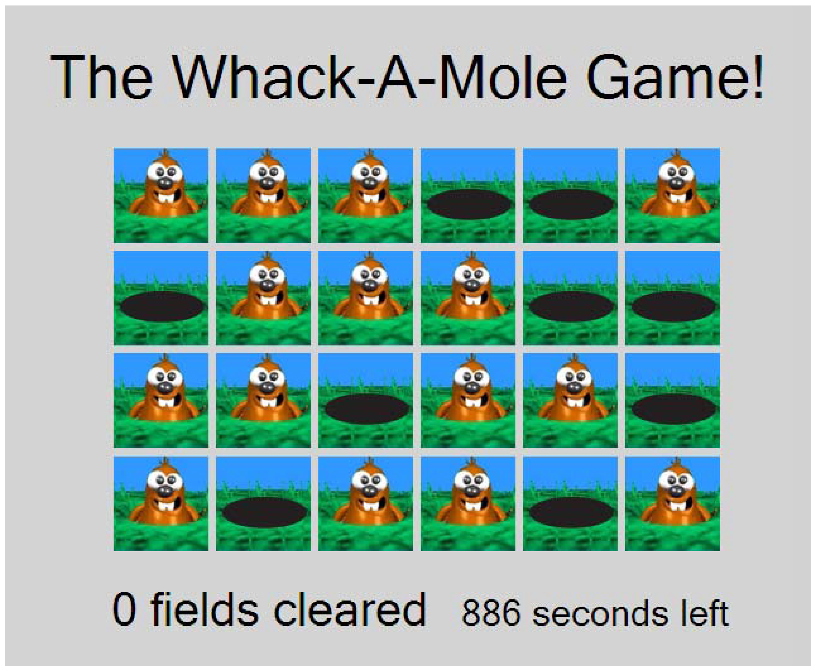
Computer screenshot of the real effort task.
Figure 1.
Computer screenshot of the real effort task.
The real effort task was called the “whack-a-mole game.”
Figure 1 shows a typical screen subjects would see during the game. There is a 6 by 4 grid of moles and holes on the field. Each time the subject mouse-clicked a mole picture the picture box would show a hole picture. If the subject clicked on a hole picture nothing would happen. The object of the game is to mouse-click all of the moles until the field is clear of moles (there is only a field of holes). Once a field is cleared the computer generates a new field of moles. Each picture box has an equal probability of being a mole picture or a hole picture, so fields are half full of moles on average.
4 The performance quota required the subject to clear a pre-specified number of fields within an announced time limit. Subjects had to meet the quota to earn the endowments that were used in the PPT or CPT game. After the time ran out for the whack-a-mole game anyone who did not meet the quota was paid $ 5 and asked to leave.
5Subjects were told that by meeting the performance quota they would earn an endowment to be used in the next part of the experiment. The decision task was revealed after the whack-a-mole stage was finished. In Treatment CH1, subjects had to clear 120 mole fields in 15 minutes to earn their $ 10 private endowments for the PPT game. In Treatment CH2, subjects had to clear 120 mole fields in 15 minutes to earn an endowment that was combined with that of another subject who met the quota and placed into a joint decision fund worth $ 40 to be used in the CPT game. Once the subjects who did not fulfill the quota left, the remaining subjects were handed instructions for the PPT game or the CPT game.
Treatment CH1 implements the PPT game with the strategy response mode for second movers whereas treatment CH2 uses strategy responses in the CPT game. Treatment CH3, CH4, and CH5 use sequential responses for first and second movers. Treatment CH3 is a PPT game whereas treatments CH4 and CH5 are CPT games.
For both PPT and CPT games subjects were randomly paired as Type X and Type Y players. After reading the instructions and listening to a scripted explanation, each subject chose a sealed envelope containing a numbered mailbox key from a box containing identical envelopes. Subjects were told that the number on the mailbox key was their private identification number. They were told the numbered key would open a numbered mailbox containing their earnings from the decision-making game plus their show-up fee of $ 5. Subjects collected their earnings one at a time, in private, and subsequently left the laboratory.
Table 1.
Summary of treatments, sample sizes, and subjects’ earnings.
Table 1.
Summary of treatments, sample sizes, and subjects’ earnings.
| Treatment | Number of Subjects | Average $ X Earned | Average $ Y Earned |
|---|
| COW1 (PPT) | 68 | 11.00 | 20.29 |
| COW2 (CPT) | 68 | 12.12 | 20.85 |
| CH1 (PPT) | 64 | 12.72 | 18.53 |
| CH2 (CPT) | 62 | 12.84 | 21.68 |
| CH3 (PPT) | 56 | 11.84 | 17.66 |
| CH4 (CPT) | 64 | 10.87 | 18.77 |
| CH5 (CPT) | 64 | 10.86 | 18.83 |
Table 1 summarizes all treatments, sample sizes, and average salient payoffs received by subjects. (The salient payoff amounts in
Table 1 do not include the $ 5 show-up fee.) The numbers of
pairs of subjects are one-half the numbers in the second column. The treatments were implemented with a between-subjects protocol (
i.e., no subject participated in more than one treatment).
6. Strategy Method Protocol Treatments
The COW study used a sequential move protocol to elicit first mover (Type X) and second mover (Type Y) decisions. The difficulty in testing Axiom S using the sequential move protocol is that only one Type Y decision is made, and the potential responses to other opportunity sets the Type X player could have offered are not observed. Type X decisions could be distributed such that all possible decisions are observed frequently or decisions could be clustered. The latter case would make a direct test of Axiom S require a very large sample under the sequential move protocol. The strategy method protocol offers the benefit of making all potential responses observable. It does this by asking a Type Y player to submit a planned response for each possible decision by a Type X player.
There are some potential problems with using the strategy method protocol. First is the reduction in incentives for Type Y players. Type Y players now have to make multiple potentially binding responses, yet only one decision determines their payoffs in the end. Their decision-making costs increase but their expected rewards do not. There is also a potential “hot” versus “cold” effect. A Type Y response in the sequential move protocol is considered “hot” because it is potentially more emotional for the Type Y player to learn the Type X player’s decision, and how the decision affects their opportunities, before responding. The strategy method protocol is considered “cold” because a Type Y subject submits a planned response without knowing the Type X decision beforehand. There is mixed evidence on the significance of hot versus cold responses. Three studies do not find a hot versus cold effect [
25,
26,
27] while two studies do find an effect [
28,
29].
Treatments CH1 and CH2 use the strategy method protocol to elicit Type Y responses, which requires 11 decisions. After the Type X and Type Y subjects in a pair make their decisions, the actual Type X decision makes the associated Type Y response to that decision binding and the game is played out to determine the money payoffs to the subjects.
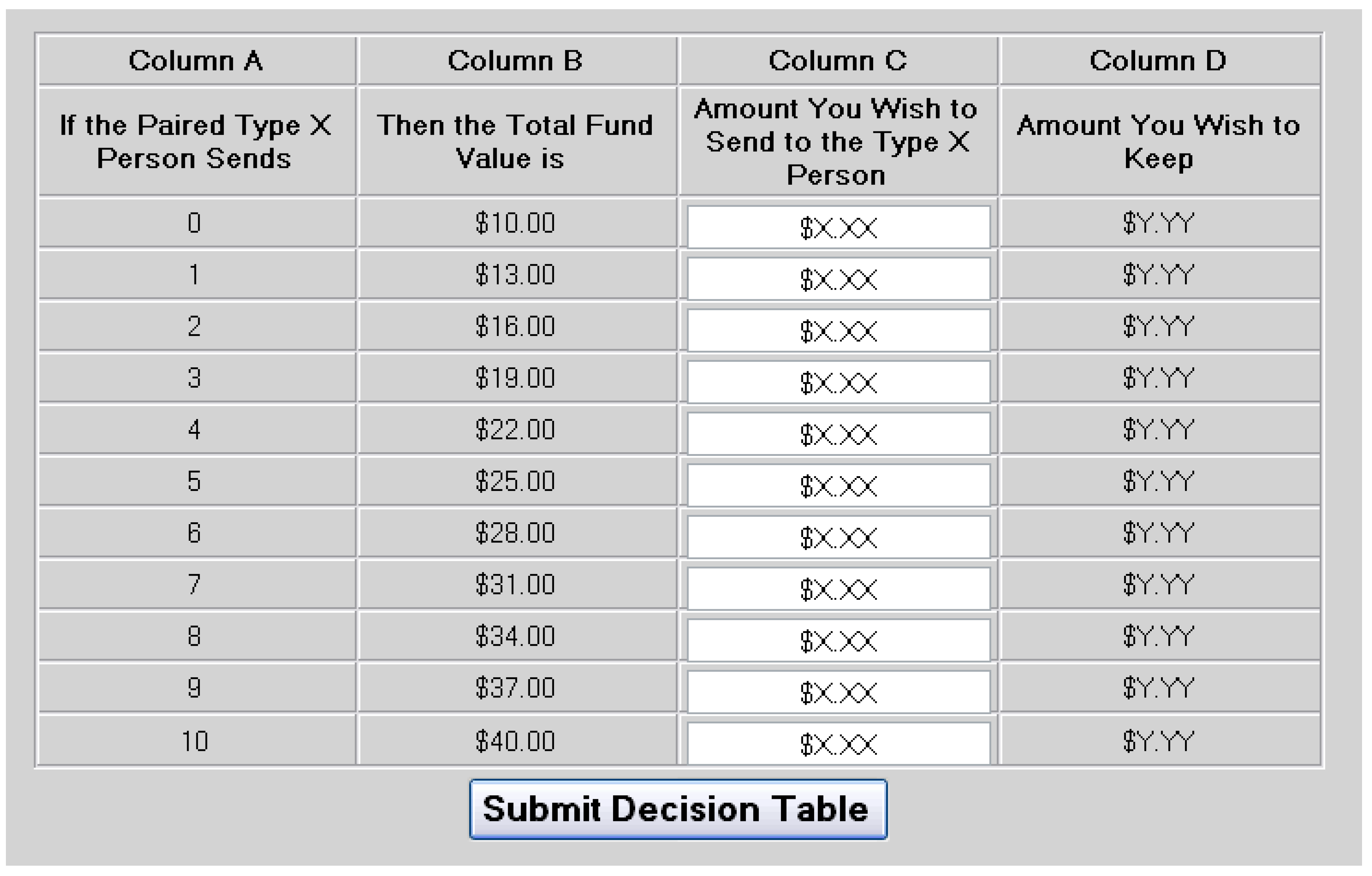
Figure 2 shows a screen shot of the Type Y player’s decision table for the PPT game with the strategy method protocol. The rows are organized by the Type X person’s potential actions in column A, with the first row representing the status quo. A subject enters an amount in each row of column C. The decisions can be entered in any order and changed at will up until the time the subject clicks on the Submit Decision Table button. The computer calculates an amount for a row in column D after a value is entered in that row of column C. The decision table for the CPT game is similar except the Type X player withdraws rather than sends so the values in column B
decrease from (the status quo amount) $ 40 to $ 10.
Figure 2.
Type Y decision screen for the strategy method protocol.
Figure 2.
Type Y decision screen for the strategy method protocol.
126 undergraduate students from Georgia State University participated in Treatments CH1 and CH2 in four sessions.
6 Treatment CH1 (the PPT game) was conducted in two sessions and, in total, 32 Type X subjects sent on average $ 5.63 and 32 Type Y subjects returned on average $ 6.96. Treatment CH2 (the CPT game) was also conducted in two sessions and, in total, 31 Type X subjects left, on average, $ 7.26 and 31 Type Y subjects returned, on average, $ 5.82. These figures are for all strategy responses by Type Y subjects.
Table A1 in the appendix shows the summary data for Treatments CH1 and CH2 using realized subject payoffs.
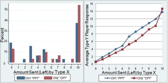
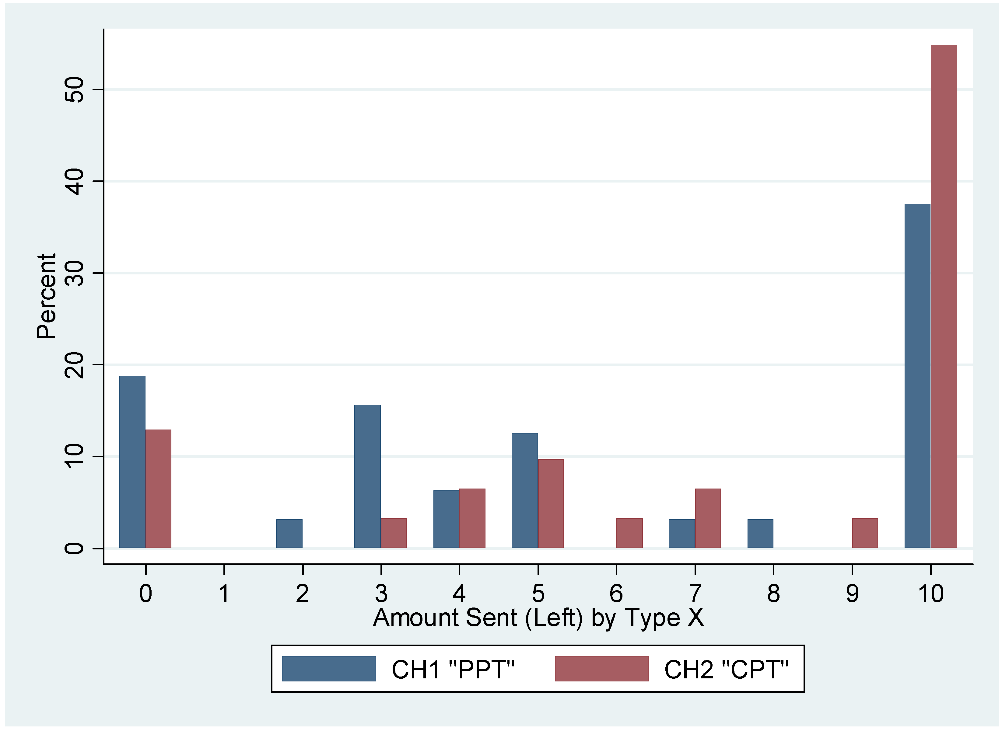
7Figure 3 compares the distributions of Type X decisions for the two games. For the PPT game there are modes at 0, 3, and 10 dollars sent, and the distribution is W-shaped with a fat right tail at 10 dollars sent. For the CPT game there are modes at 0, 5, and 10 dollars left, and the distribution is J-shaped with more than half of the subjects choosing not to withdraw anything.
Figure 3.
Comparison of Type X data for CH1 and CH2.
Figure 3.
Comparison of Type X data for CH1 and CH2.
Table 2 shows the results of parametric and nonparametric tests of Type X subject data. The mean number of dollars left in the CPT game is greater than the mean number of dollars sent in the PPT game and the difference is significant according to the t-test. The distributions of amounts sent by Type X subjects in the PPT and CPT games are
not significantly different according to the Mann-Whitney and Kolmogorov-Smirnov tests.
Table 2.
Parametric and nonparametric tests of Type X data for CH1 and CH2.
Table 2.
Parametric and nonparametric tests of Type X data for CH1 and CH2.
| | Parametric Test | Nonparametric Tests |
|---|
| Test | Means Test (t-test) | Mann-Whitney Test (Rank Sum) Test | Kolmogorov-Smirnov Test |
| Null Hypothesis | CH1 = CH2 | CH1 = CH2 | Distributions are Equal |
| Test Statistic | t = –1.7088
Pr(|T| > |t|) = 0.0924
Pr(T<t) = 0.0462* | z = –1.692
Pr > |z| = 0.0906
Pr(CH1>CH2) = 0.383 | D = 0.2399
Exact p-value = 0.256 |
The most straightforward test of hypothesis
is a two sample proportions test of the distributions of Type X responses across the 11 possible choices in the PPT and CPT treatments. This test poses the question of whether the differences in empirical frequencies shown in
Figure 3 are statistically significant. This test is reported in
Table A2 in the appendix. There is only one proportion (for amount sent or left equal to 3) that is significantly different between the PPT and CPT data at 5 percent. The absence of significance for the proportions at “no trust” and “full trust” means that the data fail to reject hypothesis
.
We now turn our attention to second mover (Type Y) data. There are 352 and 341 Type Y decisions made in Treatments CH1 and CH2, respectively. Each subject in each treatment makes 11 decisions. There is no reason to assume independence of an individual’s decisions. Our data analysis responds to this feature of the data in two ways. We report tests based on average responses across subjects to each amount that first movers could send. These average responses are independent across the 11 amounts that a first mover can send. The other way we analyze the data is with a random effects tobit estimation strategy in which an individual subject is a “panel.”
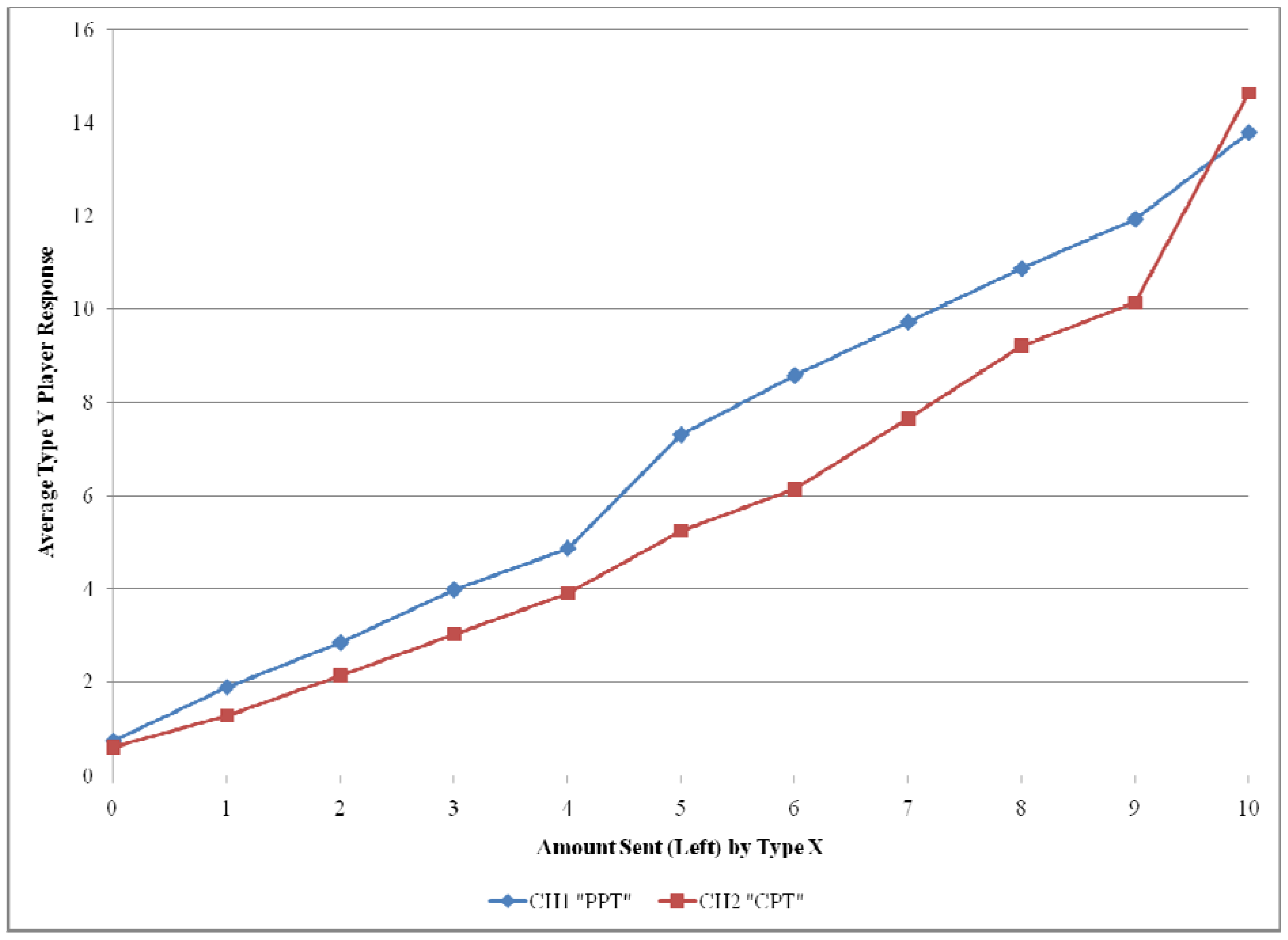
Averaging the responses across second movers for each amount that can be sent by a first mover produces the variables reported in
Figure 4 for the PPT and CPT treatments. The Type Y average across subjects is higher in the PPT treatment than the CPT treatment for all Type X choices except the extremes of 0 and 10.
Figure 4.
Comparison of average Type Y response data for CH1 and CH2.
Figure 4.
Comparison of average Type Y response data for CH1 and CH2.
Table 3 reports results from a t-test and a Wilcoxon test for matched pairs. Both tests yield a highly significant difference between second mover responses in the PPT and CPT treatments. The null hypothesis
that second movers (Type Y) will return the same amounts in the PPT and CPT games is rejected in favor of the alternative hypothesis
(implied by Axioms R and S) that second movers will return more in the PPT game.
Table 3.
Parametric and nonparametric tests of average Type Y response data for CH1 and CH2.
Table 3.
Parametric and nonparametric tests of average Type Y response data for CH1 and CH2.
| | Parametric Test | Nonparametric Test |
|---|
| Test | Means Test (t-test, paired data) | Wilcoxon Matched-Pairs Signed-Rank Test |
| Null Hypothesis | CH1 = CH2 | CH1 - CH2 = 0 |
| Test Statistic | t = 3.85
Pr(|T| > |t|) = 0.0032**
Pr(T>t) = 0.0016** | z = 2.578
Pr > |z| = 0.0099** |
This conclusion is also supported by the random effects tobit estimation with individual subject data that is reported in
Table A3 in the appendix. The coefficient on the amount sent or left by Type X players is significantly positive, which provides support for Axiom R. The common property intercept and slope dummy variables are both significant, which provides support for Axiom S. The estimated parameter for the intercept dummy variable is negative whereas the parameter for the slope variable is positive. This is consistent with: (a) second movers’ objection to any change, due to first movers’ withdrawals, from the (most generous) feasible set determined by the $ 40 common pool endowment; and (b) their willingness to reward first movers’ relative restraint in choosing smaller withdrawals.
7. Sequential Move Protocol Treatments
Why does the real effort task provide significant support for Axiom S (i.e., rejection of the null hypothesis )? The real effort task may create a stronger sense of entitlement to the endowments. When the Type X player withdraws any positive amount in the CPT game she destroys property that is not just jointly owned but now the Type Y player may have a stronger sense of entitlement to the joint fund. In other words the real effort task may create entitlements which make the property right assignments salient enough to bring Axiom S preferences out of latency.
It is natural for one to ask whether rejection of the null hypothesis can be attributed to use of the real effort task or use of the strategy method. Both design changes may affect behavior. The real effort task makes property ownership more salient. The strategy method lowers incentives because Type Y subjects have to submit 11 decisions instead of one for the same expected payoff. To get more insight we conducted sequential move treatments with the real effort task.
The experiment design and procedures for our sequential move protocol treatments are similar to the COW study except there are stronger property right entitlements. In Treatment CH3, subjects had to clear 120 mole fields in 15 minutes to play the PPT game. In Treatment CH4, subjects had to clear 120 mole fields in 15 minutes to play the CPT game. In Treatment CH5, subjects had to clear 240 mole fields in 30 minutes to earn the endowment necessary to play the same CPT game played in Treatment CH4. Treatment CH5 was conducted to set the mole-whacking effort per dollar of endowment earned equal to that in Treatments CH1 and CH3. The potential final earnings are identical in all three treatments.
184 undergraduate students from Georgia State University participated in Treatments CH3, CH4, and CH5 run in seven sessions.
8 56 subjects participated in Treatment CH3, the PPT game with a 120 mole field task. Treatment CH3 generated 28 Type X decisions (an average of $ 4.75 was sent) and 28 Type Y decisions (an average of $ 6.59 was returned). Treatment CH4, the CPT game with a 120 mole-field quota, was conducted in three sessions that generated 32 Type X decisions (an average of $ 5.28 was sent) and 32 Type Y decisions (an average of $ 6.14 was returned). Treatment CH5, the CPT game with a 240 mole-field quota, was conducted in two sessions, which generated 32 Type X decisions (an average of $ 4.84 was sent) and 32 Type Y decisions (an average of $ 5.70 was returned).
Table A4 in the appendix displays the summary statistics for these treatments.
Differences between Treatment CH4 and Treatment CH5 data are insignificant, so the Treatment CH4 and CH5 data are pooled in tests reported in the text. (The
appendix tables report separate tests for CH4 and CH5 data.) 128 subjects participated in Treatments CH4 and CH5 combined, which generated 64 Type X decisions (an average of $ 5.06 was left) and 64 Type Y decisions (an average of $ 5.92 was returned).
Table A5 in the appendix summarizes the pooled Type X and Type Y decisions from Treatments CH4 and CH5, the CPT game.
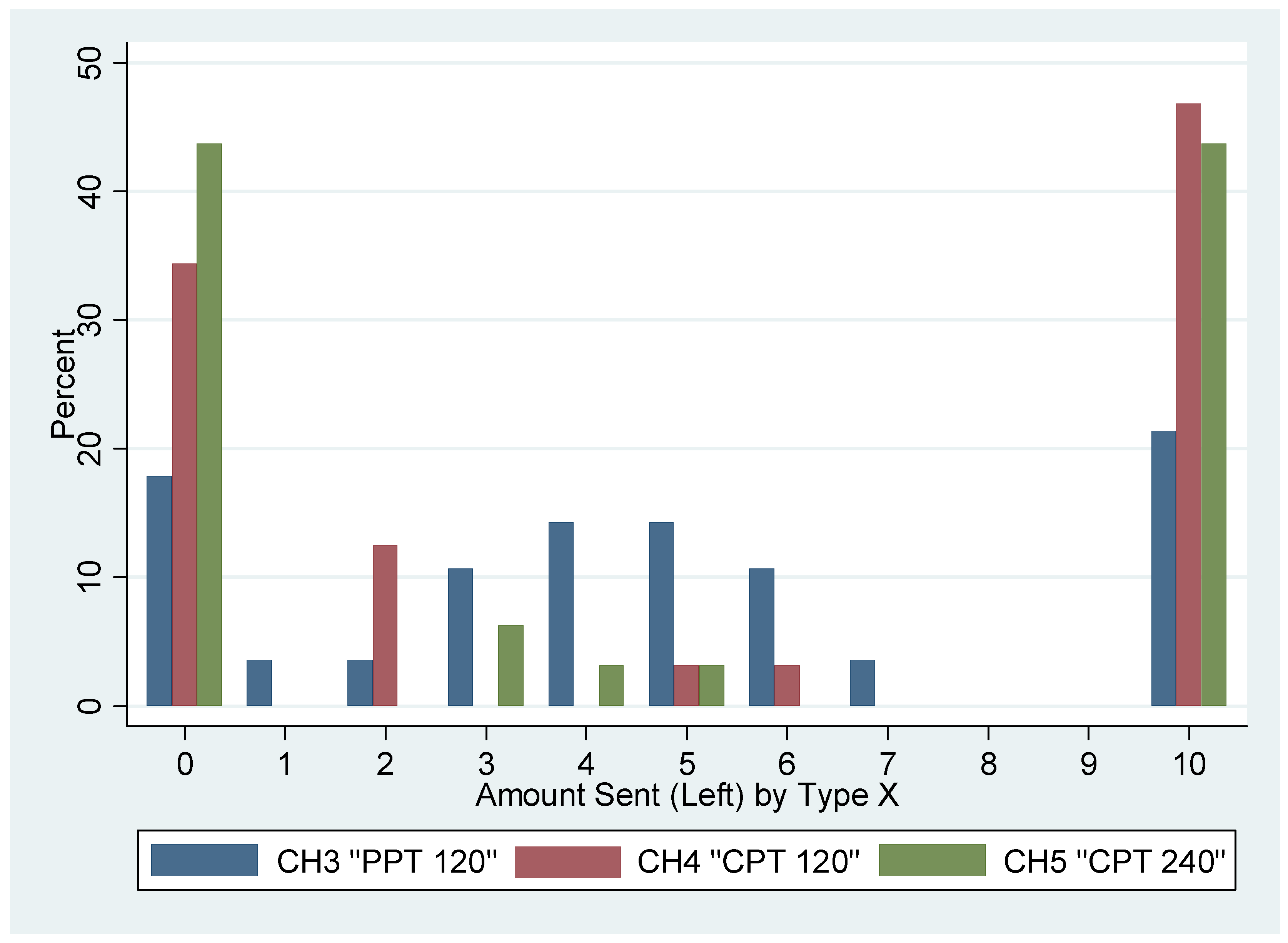
Figure 5 displays the distributions of Type X decisions in all three treatments. Treatment CH4, the PPT game, has a W-shaped distribution with modes at 0, 4, 5, and 10. Treatments CH4 and CH5, the CPT game treatments, both have U-shaped distributions with heavy modes at 0 and 10. Type X decisions move to the extremes of “full trust” and “no trust” in the CPT game much more strongly than in the PPT game. This result is more pronounced in the sequential move protocol treatments than in the strategy method treatment (compare
Figure 3 and
Figure 5).
The straightforward test of hypothesis
, the two sample proportions test of the distributions of Type X responses is reported in
Table 4. This test poses the question of whether the differences in empirical frequencies shown in
Figure 5 are statistically significant. CH3 has significantly lower proportions of observations at 0 and 10 than does pooled CH4 and CH5. In addition, CH3 has significantly higher proportions of observations at 4, 5, and 6 than does pooled CH4 and CH5. These test results support rejection of hypothesis
, that the empirical frequency distributions are the same for PPT and CPT games, in favor of the alternative hypothesis
that subjects are more likely to choose “full trust” and “no trust” in the CPT game than in the PPT game.
Table A6 in the appendix reports two sample proportions tests for CH4 and CH5 data separately; these tests support similar conclusions.
Figure 5.
Comparison of Type X data for CH3, CH4, and CH5.
Figure 5.
Comparison of Type X data for CH3, CH4, and CH5.
Table 4.
Proportions tests of Type X data for CH3 and pooled CH4 and CH5.
Table 4.
Proportions tests of Type X data for CH3 and pooled CH4 and CH5.
| Type X sent or left | Treatment CH3 (PPT) | N | Treatments CH4 & CH5 (CPT) | N | one-sided p-value |
|---|
| 0 | 0.1786 | 5 | 0.390625 | 25 | 0.0229* |
| 1 | 0.0357 | 1 | 0.0000 | 0 | 0.0642 |
| 2 | 0.0357 | 1 | 0.0625 | 4 | 0.301 |
| 3 | 0.1071 | 3 | 0.03125 | 2 | 0.0698 |
| 4 | 0.1429 | 4 | 0.015625 | 1 | 0.0066** |
| 5 | 0.1429 | 4 | 0.03125 | 2 | 0.023* |
| 6 | 0.1071 | 3 | 0.015625 | 1 | 0.0238* |
| 7 | 0.0357 | 1 | 0.0000 | 0 | 0.0642 |
| 8 | 0.0000 | 0 | 0.0000 | 0 | … |
| 9 | 0.0000 | 0 | 0.0000 | 0 | … |
| 10 | 0.2143 | 6 | 0.453125 | 29 | 0.015* |
Table A7 in the appendix reports additional parametric and non-parametric tests of Type X data. All t-tests fail to reject the null hypothesis that all treatments have similar mean amounts sent or left. The Mann-Whitney and Komolgorov-Smirnov tests imply that no distribution is significantly different from another in any treatment comparison.
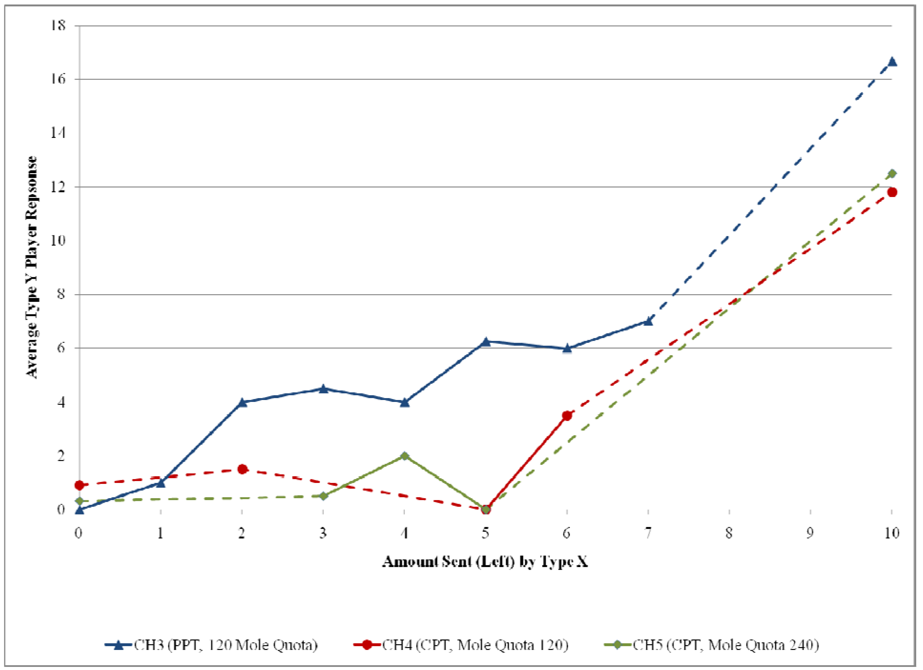
We now turn our attention to second mover (Type Y) data. Averaging the responses across Type Y subjects for each amount that can be sent by a Type X subject produces the variables reported in
Figure 6 for the PPT and CPT treatments. The dashed parts of the piecewise-linear graphs highlight parts of the response space for each treatment in which there are no observations
because there were no Type X choices that could elicit Type Y responses. For example, the dashed segment of the blue (CH3) part of the display indicates that no Type X subject sent either $ 8 or $ 9 to a Type Y subject in the CH3 treatment. Note that the PPT (Treatment CH3) graph generally lies above the two CPT (Treatments CH4 and CH5) graphs and thus reveals a similar pattern to that shown in
Figure 4 for the strategy method treatments. But the strategy method used in Treatments CH1 and CH2 elicited Type Y responses for all possible Type X choices whereas the sequential choice method used in Treatments CH3, CH4, and CH5 yields many “missing observations.”
Figure 6.
Comparison of average Type Y response data for CH3, CH4, and CH5.
Figure 6.
Comparison of average Type Y response data for CH3, CH4, and CH5.
Table 5 reports results from a paired t-test and a Wilcoxon test for matched pairs, with the sequential response data, using the same approach used for strategy response data in
Table 3. The p-value for the paired means t-test is 0.0051 and the p-value for the Wilcoxon matched pairs test is 0.0277. Similar to the strategy response data, tests of the sequential response data in
Table 5 reject
in favor of
.
Table A8 in the appendix reports the same tests comparing Treatment CH3 to Treatments CH4 and CH5 separately; these tests support similar conclusions.
Table 5.
Parametric and nonparametric tests of avg. Type Y data for CH3 and pooled CH4 and CH5.
Table 5.
Parametric and nonparametric tests of avg. Type Y data for CH3 and pooled CH4 and CH5.
| | Parametric Test | Nonparametric Test |
|---|
| Test | Means Test (t-test, paired data) | Wilcoxon Matched-Pairs Signed-Rank Test |
| Null Hypothesis | CH3 = (CH4 & CH5 pooled) | CH3 – (CH4 & CH5 pooled) = 0 |
| Test Statistic | t = 2.491
Pr(|T| > |t|) = 0.0674
Pr(T>t) = 0.0051** | z = 1.461
Pr > |z| = 0.0277* |
Table A9 in the appendix reports three tobit random effects estimations with Type Y return amounts as the dependent variable using data from Treatments CH3, CH4, and CH5. The independent variables include the Type X amount sent or left and CPT game intercept and slope dummy variables. The Type Y data are consistent with Axiom R as indicated by the “Type X Sent or Left” variable’s statistical significance. The data do not support a strict preference version of Axiom S, as indicated by the insignificance of both the CPT Intercept and Slope dummy variables. The lack of significance is likely coming from differences in the distribution of Type X decisions between the PPT and CPT games. Roughly 1/3 of all Type X decisions are to send $ 0 or $ 10 in the PPT game whereas to 2/3 of all Type X decisions are to withdraw $ 0 or $ 10 in the CPT game. The modal Type Y response to $ 0 sent ($ 10 withdrawn) is to return (leave) $ 0. When $ 10 are sent in the PPT game, the average return is $ 16.67 (standard deviation 8.16), and when $ 0 are withdrawn in the CPT game the average return is $ 12.14 (standard deviation 8.23).
Tests of COW data with the same approach used in
Table 5 and appendix
Table A9 produce insignificant differences between the PPT and CPT treatments reported in the COW paper, confirming the tests results reported therein.
Support for both and is found in the sequential move protocol treatments. The entitlements appear to be not only salient enough to bring Axiom R and S preferences out of latency, but also salient enough for Type X players to anticipate these preferences and respond accordingly by choosing the extremes of “full trust” and “no trust.”

