Cournot’s Oligopoly Equilibrium under Different Expectations and Differentiated Production

Abstract

The subject of this study is an oligopolistic market in which three firms operate in an environment of quantitative competition known as the Cournot oligopoly model. Firms and their production are differentiated, which brings the theoretical model closer to real market conditions. The main objective was to expand the Cournot duopoly and add another firm, resulting in an oligopolistic market structure assuming a partially differentiated production and coalition strategy between two firms. This article contains an oligopolistic model specifically designed for three different types of expectations, and has been applied to find and verify the stability of the net equilibrium of oligopolists. The market of telecommunication operators in Slovakia was selected as a real market case with accessible data on an oligopoly with three companies and partial differentiation. There are studies in which the authors limit their considerations to a certain number of repetitions of oligopolistic games. An infinite time interval is considered here. Three types of future expectations were considered: a simple dynamic model (or naïve expectations) in which the oligopolist assumes that its competitors will behave in the future based on their response functions, an adaptive expectations model in which the oligopolist considers a weighted average of the quantities offered by its competitors, and real expectations in which firms behave as rational players and do not have complete information about demand and offer output based on expected marginal profit. While the presented model proved to be stable under naïve and adaptive expectations, no stable equilibrium was found under real expectations and further results indicate a chaotic behavior.

1. Introduction

Microeconomic theory recognizes two extreme cases of market structures, namely the market structure of monopoly and the market structure of perfect competition. A duopolistic and then oligopolistic market can be considered as the initial stage of transition from a monopoly to a market with perfect competition. The analytical expression of oligopoly is more complex than the market extremes mentioned above. This complexity arises from the fact that a firm operating in an oligopolistic market must take into account not only the behavior of consumers, as reflected in the market demand curve, but also the behavior of its competitors, including their response to any significant actions that affect their market position.

The subject of this study is an oligopolistic market in which three firms operate in an environment of quantitative competition known as the Cournot oligopoly model. The firms and their production are differentiated, i.e., each of the firms uses its own production processes and technologies (resulting in different cost functions), and production is not homogeneous. This assumption brings the theoretical model closer to real market conditions, since there are rarely firms whose output is completely homogeneous, i.e., whose products are perfect substitutes. Simultaneously, it was assumed that the products are not perfectly complementary, but also not perfectly independent.

The assumptions of the classical Cournot model can be considered unrealistic under today’s market conditions. It assumes that players set their quantity independently. Since there are only a limited number of players, they would usually react very strongly to the strategies of their competitors. Under real market conditions, competition is not only based on quantity and price, but also on differentiation. The models presented in this article eliminate these shortcomings of the original Cournot model to a considerable extent.

The main objective is to extend the well-known model of duopoly—the Cournot duopoly—by another firm leading to an oligopolistic market structure under the assumption of a partially differentiated production and coalition strategy between two firms, which could bring the theoretical model even closer to real market conditions and show new perspectives for oligopolistic market strategies.

As firms adjust their decisions over time based on different expectations of future performance, the goal is to find and verify the stability of the oligopolists’ net equilibrium. The Slovak mobile network operators (MNO) market was chosen to demonstrate the application of the developed models. The presented models consider three types of expectations, i.e., naïve, adaptive, and real expectations.

This article has the following structure. The introduction contains the identification and description of the research subject, the underlying theory and general assumptions, the description of the Cournot oligopoly model and the possibilities of oligopolists to adapt over time. The subsection on the underlying theory also contains the derivation of the inverse demand functions and general assumptions regarding the model variables that were further applied. The second subsection of the introduction presents the Cournot oligopoly model as a basis for further modifications. The last subsection of the introduction describes the firm’s adaptation to new market situations, including naïve, adaptive, and real expectations of firms. The second section is entitled Proposed model modifications and presents proposed extensions and modifications of the basic oligopoly model, aimed at incorporating differentiation of output and firms, cartelization of the oligopoly by two players and entry of a new firm. It involves the derivation of static quantities and prices of the oligopolists and the adjustment of firm decisions by defining and applying naïve, adaptive, and real expectations about the future market situation. We show the dynamic map for each type of expectation and also eight fixed points of the dynamic map for real expectations. In the Results section, we present the numerical solution of the proposed model for the case of the Slovak mobile operators’ market. This section starts with the naïve expectations, where the results are the same as for the static model, then continues with the results for the adaptive expectations, where a stable solution was found, and finally with the results for the real expectations, where only one of the fixed points gives a non-negative quantity for all three firms. The discussion section discusses the stability of the equilibria found under all three types of expectations when the exogenous parameters change. The conclusion summarizes the results presented and points the way for future research.

1.1. Underlying Theory and General Assumptions

Since equilibrium in an oligopolistic market depends on multiple decisions of several firms, the optimal strategy is obtained by solving a system of equations. If one considers the time factor and assumes an equilibrium that changes in the course of time, this system of equations is described and solved as a dynamic system. Verhulst [1] explains that a dynamic system is based on the evolution of “something” over time. In creating a dynamic system, it is necessary to decide what is “something” that evolves over time and what is the rule that describes how it behaves over time. Thus, the dynamic system could be defined as a model that describes the evolution of the system over time. The first step in creating a dynamic system is to decide which developments to track over time. For this purpose, the variables that affect the model and describe the state of the system at each point in time should be defined. The variables that describe the state of the system are called the state variables, and the set of all possible values of these variables is called the state space. The next step in creating a dynamic system is to define the rules for how the system will evolve over time. These rules must be defined in such a way that the state variables completely describe the state of the system, i.e., the value of state variable at a certain point in time must completely describe the development of all future states.

Thus, the state space determines what values the state vector of a dynamic system can take. A state vector consists of a set of variables which can take values from a certain interval. A state space can be finite with a limited number of states in which a dynamic system can be found, countable with an infinite but countable number of states, i.e., natural numbers can be assigned to each state, or infinite with real numbers as state variables, i.e., it is not only infinite but also not computable [2].

Scheinerman [3] presents the mathematical formulation of a discrete dynamic system as follows: a dynamic system is specified by a state vector $xϵ{ℝ}^n$ and a function $f:{ℝ}^n\to {ℝ}^n$, which describes how the system evolves over time. A discrete dynamic system can be described by equations $x\left(0\right)=x_0$ a $x\left(t+1\right)=f\left(x\left(t\right)\right)$. It follows that $x\left(t\right)=f^t\left(x_0\right)$ represent t-th application f to $x_0$. For a given dynamic system $x\left(t+1\right)=f\left(x\left(t\right)\right)$ and the initial condition $x_0$, p and we want to find the value $x\left(t\right)$ at all times t.

In the case of dynamic equilibrium for a number of entities larger than two, instability of the obtained solution may occur [4]. In several studies [5,6], the authors state that it is possible to divide consumers into groups based on their behavior, where it is possible to create a so-called representative agent (consumer) who buys the products of the analyzed oligopolists. The utility function of such a consumer could be expressed as

$$U\left(q_i, \mathit{I}\right)={\displaystyle \sum }_{i=1}^n{\alpha }_i{q}_i-\frac{1}{2}\left({\displaystyle \sum }_{i=1}^n{q}_i^2+2\gamma {\displaystyle \sum }_{i=1}^n{\displaystyle \sum }_{j>i}^n{q}_i{q}_j\right)-I$$

(1)

where

$q_i$—quantity of purchased goods,

$I={\displaystyle \sum }_{i=1}^n{p}_i{q}_i$,

$p_i$—price of the i-th product,

${\alpha }_i$—coefficient measuring the quality of the i-th consumed product, and

$\gamma$—coefficient measuring the degree of product differentiation.

This study considers an oligopoly model with three firms whose inverse demand functions (price–sales) are linear and can be expressed in the following form:

$$p_k={\alpha }_k-q_k-\gamma {{\displaystyle \sum }}_{l\ne k}^3{q}_l, k=1, 2, 3$$

(2)

where

$p_k$—the production price of the k-th company,

$q_k$—the production volume of the k-th company, and

${\alpha }_k$—coefficient measuring the quality of production of the k-th company.

• Assumption 1.

$\left|\gamma \right|<1$the products of oligopolists are neither perfect substitutes nor complements,

$\gamma \ne 0$the production of oligopolists is interdependent, and

Note: If $\gamma =1$ or $\gamma =-1$, products of oligopolists are perfect substitutes, complements.

If Equation (2) is modified for three firms, the production of each oligopolist can be derived and thus the demand functions for oligopoly products can be obtained.

$$\begin{gathered} q_1=\frac{\left({\alpha }_1-p_1\right)\left(1+\gamma \right)-\gamma \left[({\alpha }_2-p_2)+\left({\alpha }_3-p_3\right)\right]}{\left(1-\gamma \right)\left(1+2\gamma \right)} \\ {q}_2=\frac{\left({\alpha }_2-p_2\right)\left(1+\gamma \right)-\gamma \left[({\alpha }_1-p_1)+\left({\alpha }_3-p_3\right)\right]}{\left(1-\gamma \right)\left(1+2\gamma \right)} \\ {q}_3=\frac{\left({\alpha }_3-p_3\right)\left(1+\gamma \right)-\gamma \left[({\alpha }_1-p_1)+\left({\alpha }_2-p_2\right)\right]}{\left(1-\gamma \right)\left(1+2\gamma \right)} \end{gathered}$$

(3)

The demand Function (3) should be set as non-negative, i.e., consumers do not buy negative quantities of oligopolist output. Therefore, both the numerator and denominator must be positive or negative. Under Assumption 1, the denominator is always positive. To ensure that the demand functions are not negative, the following are placed on the parameter values:

$$\begin{gathered} {\alpha }_1\left(1+\gamma \right)-\gamma \left({\alpha }_2+{\alpha }_3\right)>0 \\ {\alpha }_2\left(1+\gamma \right)-\gamma \left({\alpha }_1+{\alpha }_3\right)>0 \\ {\alpha }_3\left(1+\gamma \right)-\gamma \left({\alpha }_1+{\alpha }_2\right)>0, \end{gathered}$$

We can rewrite these rules in a more common notation as $\underset{i=1,2,3}{\min }\left\{\frac{{\alpha }_i}{{{\displaystyle \sum }}_{j\ne i}{\alpha }_j}\right\}>\frac{\gamma }{1+\gamma }$. From this notation, we can see that for:

$\gamma <0$ the right side of this inequality is negative, so that the condition holds for all values of $\alpha$ for three firms,

$\gamma >0$ the right sight is positive and increasing in $\gamma$, and

$\gamma =1$ the right-hand side is equal $\frac{\gamma }{1+\gamma }=\frac{1}{2}$, what means for $\gamma <1$ we have $\frac{\gamma }{1+\gamma }<\frac{1}{2}$.

From the above, it is clear that if the products are identical in terms of product quality (case ${\alpha }_1={\alpha }_2={\alpha }_3$), the left-hand side of the inequality $\underset{i=1,2,3}{\min }\left\{\frac{{\alpha }_i}{{{\displaystyle \sum }}_{j\ne i}{\alpha }_j}\right\}>\frac{\gamma }{1+\gamma }$ is equal to $\frac{1}{2}$, so the condition holds for all values of $\gamma <1$. However, if there are differences in products quality (there are differences in the values of $\alpha$’s), the left-hand side is less than $\frac{1}{2}$. In this case, the condition will not be satisfied for sufficiently large values of $\gamma$.

For satisfying Assumption 1:

-

The three products are not too different from each other in terms of quality and/or

-

The products are not extremely substitutable for each other.

• Assumption 2.Firms have linear cost functions with a zero constant, i.e., their marginal costs ($M{C}_k$, $k=1, 2, 3$) are constant for any quantity of output. To exclude negative output, rule$M{C}_k>0$and${\alpha }_k-M{C}_k>0, k=1,2,3$was applied. The second inequality represents the net quality of the firm’s output [7].

1.2. Cournot Oligopoly Model

The equilibrium, as described by Cournot [8], represents the initial basis for the Nash equilibrium [9]. Friedman [10] states that Cournot was the predecessor of Nash. He claims that “Cournot vaguely perceived the Nash equilibrium but did not quite see it” [10] p. 39. The Nash equilibrium is most applicable to a game with complete information without repetition. When firms compete in the market repeatedly, over a long period of time, or have incomplete information, the basic Nash equilibrium must be reformulated [11].

To find the Nash equilibrium, Gibbons [12] assumed the existence of n firms in the market, each of which chooses its strategy $a_i$ from a set of feasible strategies $A_i$. The strategy may be a single variable (price, quantity, or investment in research and development), or a vector of variables. Let us assume that the payoff function represents the profit of the firm ${\pi }_i$ as a function of the strategies of other firms ${\pi }_i={\pi }_i\left(a_1, a_2\cdots a_n\right)$. The payoff function encompasses the market environment in which the firm finds itself and contains all the important information about demand, costs, and other variables. The Nash equilibrium in such a market occurs when each firm chooses its optimal strategy, while knowing the strategies of other firms. The Nash equilibrium could be described using an n-dimensional vector of strategies $\left(a_1^{*}, a_2^{*}, \cdots , a_n^{*}\right)$, where each firm i earns the maximum profit given by the strategies of the other n-1 firms $a_{-i}^{*}$, while $a_{-i}^{*}$ is a vector of other strategies of n-1 firms. This means that ${\pi }_i\left(a_i^{*}, a_{-i}^{*}\right)\ge {\pi }_i\left(a_i, a_{-i}^{*}\right)$ applies for each firm for all feasible strategies $a_i\in A_i$. The Nash equilibrium is often described by response functions.

The Nash equilibrium is such a solution where if one of the players does not adhere to his optimal strategy while his opponent does, his profit is reduced (in the best case it remains the same), i.e., whoever deviates from the optimal strategy cannot achieve a higher profit.

In formulating the Nash equilibrium for a recurrent decision situation, we discuss the so-called subgame perfect equilibrium. The subgame perfect equilibrium represents the formulation of the Nash equilibrium in dynamic games. In such games, firms choose $a_{it}$ strategies at each point in time $t=1, 2, \cdots ,T$. The players’ strategy is the subgame perfect equilibrium, which represents the Nash equilibrium in the subgame of the original game. The subgame formulation used in oligopolistic models was used in [13], and several other authors have used it in their work.

In the case of subgame perfect equilibrium, the firm makes decision $a_{it}$ at each time t based on the market trends in the past $h_t$, which includes information about all past decisions made by other firms in the market. The firm’s strategy in the case of a repeated game is then the rule ${\sigma }_i$, applied to the choice of decisions $a_{it}$ at each point in time based on the previous market behavior, which can be written as $a_{it}={\sigma }_i\left(h_t\right)$. Applying the standard Nash equilibrium approach, an equilibrium in the repeated game is simply n strategies $\left({\sigma }_1^{*}, {\sigma }_2^{*}, \cdots {\sigma }_n^{*}\right)$ such that each firm´s strategy ${\sigma }_i^{*}$ is optimal given the strategies ${\sigma }_{-i}^{*}$ of the other firms, i.e., no firm can improve its profit by choosing a different strategy, given the strategies of the other firms [11].

The main criticism of using the standard Nash equilibrium in repeated games is that it allows firms to make “threats” that are not credible, in the sense that it would not be in their interest to carry out the threat. Subgame perfection was formulated to restrict firms to credible strategies. The basic idea of subgame perfection according to Dixon [11] is quite simple. In a Nash equilibrium, the firm chooses its strategy ${\sigma }_i$ “once and for all” at the beginning of the game and remains committed to it throughout the game. To eliminate non-credible threats in a subgame-perfect equilibrium, firms choose their strategy at each point for the rest of the game. The “subgame” at any time t is simply the remainder of the game from t until the last period T. Subgame perfection requires that the strategies chosen in each subgame are Nash equilibria. This rules out non-credible threats, since a firm must choose its strategy optimally at each stage of the game.

When we consider incomplete information in the search for an optimal oligopoly strategy, we look for what is so-called a sequential equilibrium. This equilibrium represents the Nash equilibrium for an extensive form of the game. The sequential equilibrium specifies not only specify the strategy of the players, but also their estimates of the moves of other players [14]. The firms do not know the exact form of the other players’ payment functions in this type of game; they can only estimate them based on the available information (e.g., they do not have information about the other firms’ costs or objectives). In the first phase of the game—at the beginning—the firms have some initial ideas about the behavior of the other firms, which they can adjust as the game progresses. It means that firms can “learn” something about their competitors based on their past decisions. In this case, for example, a firm can strengthen its position by making decisions that are different from those made by other firms. Milgrom and Roberts [15] note that lower-cost incumbents can differentiate themselves from higher-cost incumbents through a low-cost strategy, which is inefficient, sometimes even liquidating, for high-cost firms. In this equilibrium, low-cost firms sacrifice their immediate profits for higher future profits—they expect high-cost firms to exit the market. In another way, de Frutos, Gatón, and Novo [16] study a discrete-time semidiscretization of a non-cooperative differential game with infinite time horizon for N-players.

The Nash equilibrium is used in oligopoly theory for several reasons. One is that if firms make their own decisions, they have no reason to deviate from the equilibrium. The second reason is that firms that anticipate the Nash equilibrium choose a strategy based on that equilibrium because that decision is their best response to the anticipated strategies of the other firms [11]. As we have already noted with the Cournot equilibrium, the Nash equilibrium does not always exist, or we can find multiple equilibrium points.

To clarify the relationship between the Cournot equilibrium (formulated in 1838) [11] and the Nash equilibrium (formulated in 1951) [11], both of which are used in oligopoly models, we use the idea of R.B. Myerson: “We can speak of Cournot as the founder of oligopolistic theory, but attributing the discovery of the fundamental concept of solving the theory of non-cooperative games to him would be a replacement of the method application with its general formulation.” [11]. This means that Cournot and later Nash had the same ideas. However, Cournot did not try to formulate a general solution beyond the model he considered, which Nash did in his work. Moreover, the formulation of oligopoly through game theory is more appropriate. Based on the same idea, some authors refer to the equilibrium of non-cooperative oligopolies as Nash–Cournot or Cournot–Nash equilibrium (e.g., [11] and later other authors).

1.3. Adaptation Possibilities of Oligopolists over Time

Currently, there is increasing research on how oligopolists adapt to new circumstances. In this article, we will address adaptation models in the case of the Cournot oligopoly model, but nevertheless provide at least a brief overview of the authors who have studied the oligopoly adaptation model.

For example, Ahmed and Agiza study adaptive expectations in their model [11], where oligopolists express their expectations of future developments based on past developments (previous states of the system), considering a dynamic system for n firms and studying the stability of the equilibrium found. Agiza, Bischi and Kopel [11] later reported the stability of an oligopoly model with three homogeneous firms. Huang [11] notes that there has been much recent pressure to use chaos theory in economic models. Although chaos models are used in science and engineering, their application to economic models is complex. For this reason, he recommends adaptation models as an effective tool for stabilizing chaotic processes.

Authors relying on the Kopel model [17] assumed homogeneous expectations of firms and showed a space for model parameters and initial assumptions in which the model converges to the Nash equilibrium.

Agiza and Elsadany [18] consider the mixed expectations of duopolists, who assume that one firm has so-called naive expectations and the second is the so-called rational firm. For this case, they show that the model generates more chaotic trajectories than in the case of the model with homogeneous rational expectations of both firms.

The concept of adaptive rational equilibrium was introduced by Brock and Hommes [19]. In this equilibrium, firms base their decisions on predictions about the future values of endogenous variables, whose present values are determined by equilibrium equations. The predictions are based on the selection from a finite set, P, of so-called predictors or expectations containing information about past developments. In their decision making, firms use a discrete decision model according to [20,21] for the selection of the expectation function from the set P, where the deterministic part of the predictor utility is a measure of performance. Such a result represents the dynamics of the predictor selection (expectation function) associated with the dynamic equilibrium of the endogenous model variables.

Another type of oligopolist response is a chaos-based response [22], where firms do not use an autoregressive rule in their selection but select coefficients that satisfy the basic rules of chaos dynamics. One part of the dynamics of oligopolistic models has not yet been mentioned is the transition from an oligopolistic market structure to a monopoly and vice versa. This idea was introduced by Bain [23], who states that in any sector there can be a critical level of concentration where a qualitative change means the formation of cartels or natural monopolies. For business managers, it is a matter of finding and identifying the possibilities of competitors’ behavior and the point at which a qualitative shift no longer occurs.

2. Proposed Model Modifications

When oligopolistic firms search the market for a volume of output that maximizes their profits, we speak of the so-called Cournot equilibrium. Firms solve the following maximization problem under otherwise unchanged conditions [24]:

$$\begin{gathered} {\pi }_k=\left(p_k-M{C}_k\right)q_k\to max \\ {p}_k={\alpha }_k-q_k-\gamma {{\displaystyle \sum }}_{l\ne k}^3{q}_l k=1, 2, 3. \end{gathered}$$

(4)

The necessary first-order condition for the existence of an extreme of the profit function for the three oligopolists has the following form

$$\begin{gathered} \frac{d{\pi }_1}{d{q}_1}=0\to {\alpha }_1-2q_1-\gamma \left(q_2+q_3\right)-M{C}_1=0\to q_1=\frac{{\alpha }_1-M{C}_1-\gamma \left(q_2+q_3\right)}{2} \\ \frac{d{\pi }_2}{d{q}_2}=0\to {\alpha }_2-2q_2-\gamma \left(q_1+q_3\right)-M{C}_2=0\to q_2=\frac{{\alpha }_2-M{C}_2-\gamma \left(q_1+q_3\right)}{2} \\ \frac{d{\pi }_3}{d{q}_3}=0\to {\alpha }_3-2q_3-\gamma \left(q_1+q_2\right)-M{C}_3=0\to q_3=\frac{{\alpha }_3-M{C}_3-\gamma \left(q_1+q_2\right)}{2}. \end{gathered}$$

(5)

The necessary condition of the second order for the existence of the extreme of the function is satisfied for all the companies $\frac{d^2{\pi }_k}{d{q}_k^2}<0, k=1, 2, 3$. Function (5) form the oligopolists’ response functions, which can also be written as $q_1=r_1\left(q_2, q_3\right)$, $q_2=r_2\left(q_1, q_3\right)$, $q_3=r_3\left(q_1, q_2\right).$

We obtain the optimal volume of production that firms will offer in the market in the case of a Cournot equilibrium by simultaneously solving Equation (5). We obtain the optimal production volume in the case of a Cournot equilibrium by solving these equations for q_i.

$$\begin{gathered} q_1^C=\frac{\left({\alpha }_1-M{C}_1\right)\left(2+\gamma \right)}{\left(2-\gamma \right)\left(2+2\gamma \right)}-\frac{\mathsf{\gamma }\left[\left({\alpha }_2-M{C}_2\right)+\left({\alpha }_3-M{C}_3\right)\right]}{\left(2-\gamma \right)\left(2+2\gamma \right)} \\ {q}_2^C=\frac{\left({\alpha }_2-M{C}_2\right)\left(2+\gamma \right)}{\left(2-\gamma \right)\left(2+2\gamma \right)}-\frac{\mathsf{\gamma }\left[\left({\alpha }_1-M{C}_1\right)+\left({\alpha }_3-M{C}_3\right)\right]}{\left(2-\gamma \right)\left(2+2\gamma \right)} \\ {q}_3^C=\frac{\left({\alpha }_3-M{C}_3\right)\left(2+\gamma \right)}{\left(2-\gamma \right)\left(2+2\gamma \right)}-\frac{\mathsf{\gamma }\left[\left({\alpha }_1-M{C}_1\right)+\left({\alpha }_2-M{C}_2\right)\right]}{\left(2-\gamma \right)\left(2+2\gamma \right)}, \end{gathered}$$

(6)

where index $C$ represents the basic Cournot model. The price at which the oligopolists offer their output on the market is then

$$\begin{gathered} p_1^C=\frac{\left({\alpha }_1+M{C}_1\right)\left(2+\gamma \right)-2M{C}_1{\gamma }^2}{\left(2-\gamma \right)\left(2+2\gamma \right)}-\frac{\mathsf{\gamma }\left[\left({\alpha }_2-M{C}_2\right)+\left({\alpha }_3-M{C}_3\right)\right]}{\left(2-\gamma \right)\left(2+2\gamma \right)} \\ {p}_2^C=\frac{\left({\alpha }_2+M{C}_2\right)\left(2+\gamma \right)-2M{C}_2{\gamma }^2}{\left(2-\gamma \right)\left(2+2\gamma \right)}-\frac{\mathsf{\gamma }\left[\left({\alpha }_1-M{C}_1\right)+\left({\alpha }_3-M{C}_3\right)\right]}{\left(2-\gamma \right)\left(2+2\gamma \right)} \\ {p}_3^C=\frac{\left({\alpha }_3+M{C}_3\right)\left(2+\gamma \right)-2M{C}_3{\gamma }^2}{\left(2-\gamma \right)\left(2+2\gamma \right)}-\frac{\mathsf{\gamma }\left[\left({\alpha }_1-M{C}_1\right)+\left({\alpha }_2-M{C}_2\right)\right]}{\left(2-\gamma \right)\left(2+2\gamma \right)}. \end{gathered}$$

(7)

Subtracting Equation (7) from Equation (6), we obtain $p_k^C-q_k^C=M{C}_k, k=1, 2, 3$, after adjustment $p_k^C-M{C}_k=q_k^C, k=1, 2, 3$, and substituting the profit function of the oligopolists, we obtain their maximum profit at the optimal output level ${\pi }_1^C={\left(q_1^C\right)}^2, {\pi }_2^C={\left(q_2^C\right)}^2, {\pi }_3^C={\left(q_3^C\right)}^2.$

The above model is well known and generally accepted. In the following subsections, the version of the model presented above is modified and extended by assuming a situation in which two firms form a coalition against a new firm entering the market (Section 2.1) and by considering the types of future expectations that determine firms’ decision making, i.e., naïve, adaptive and real expectations (Section 2.2).

2.1. Cartel Oligopoly Model

There are several authors who focus their research on coalitional or cartel-oligopoly equilibria. For example, [25] has analyzed cartelization in Cournot competition with asymmetric costs. Bimonte, Romano and Russolillo [26] used Cournot competition as an incentive in a circular economy. Cartelization as a two-stage simultaneous game can be found in [27]. Kupies and Olaizola [28] addressed cartelization from a dynamic perspective. They also made a literature review on cartel stability and showed that the dynamic process converges to a strongly stable cartel when one exists. Later, in [29], the authors revisited the problem of cartel stability in a linear symmetric Cournot oligopoly by assuming that any coalition of firms defecting from a cartel can choose its quantity before the remaining firms. The cartel and its stability in an open and closed loop equilibrium is presented in [30].

In this article, we consider an oligopoly model with three firms, as described in the previous section. We assume a situation, where two firms form a coalition (${\pi }_c={\pi }_1+{\pi }_2$) against the last firm. For this model, we later assume naïve, adaptive, and real expectations of the oligopolists.

This model could be formulated as follows:

$$\begin{gathered} {\pi }_c={{\displaystyle \sum }}_1^k\left(p_k-M{C}_k\right)q_k\to max \\ {p}_k={\alpha }_k-q_k-\gamma {\displaystyle \sum }_{l\ne k}^2{q}_l k=1, 2 \\ {\pi }_3=\left(p_3-M{C}_3\right)q_3\to max \\ {p}_3={\alpha }_3-q_3-\gamma \left(q_1+q_2\right) \end{gathered}$$

(8)

From the necessary first-order condition for the existence of an extreme of the profit function, the response function for all firms could be derived in the form

$$\begin{gathered} q_1=r_1\left(q_2, q_3\right)=\frac{{\alpha }_1-M{C}_1-\gamma \left(2q_2+q_3\right)}{2} \\ {q}_2=r_2\left(q_1, q_3\right)=\frac{{\alpha }_2-M{C}_2-\gamma \left(2q_1+q_3\right)}{2} \\ {q}_3=r_3\left(q_1, q_2\right)=\frac{{\alpha }_3-M{C}_3-\gamma \left(q_1+q_2\right)}{2}. \end{gathered}$$

(9)

2.2. Naïve, Adaptive, and Real Expectations

It is possible to assess whether the equilibrium reached in an oligopolistic model is stable over time. From the dynamics point of view, it is necessary to introduce the future expectations of the oligopolists into the static equilibrium already considered—the assumption of future competitive behavior. There are studies in which the authors restrict their considerations to a certain number of repetitions of oligopolistic games [31,32], but in our analysis, an infinite time interval is considered, i.e., the number of games is not limited. We consider three types of future expectations for the Cournot model. The first is a simple dynamic model (or naïve expectations) in which the oligopolist assumes that its competitors will behave in the future based on their response functions [33,34]. The second dynamic Cournot model is an adaptive expectations model, where we assume that the oligopolist will consider in the future a weighted average of the quantities offered by its competitors in the previous period based on their response functions [4]. In the last model, we assume the so-called real expectations, where firms behave as rational players and do not have complete information about the market demand function and offer output quantity based on the expected marginal profit ($\frac{\partial {\pi }_i}{\partial q_i}$) [29].

2.2.1. Naïve Expectations

In studying the dynamics of firms’ response to a change in a competitor’s quantity or price, a simplifying assumption must be made, namely, that firms do not respond to a change in output or price, i.e., that their quantities offered remain the same as in the case of static equilibrium. This is called a naïve expectation. In the case of simultaneous decision making, this assumption is accepted by all firms and their dynamic response functions represent a system of dynamic linear equations—a dynamic map.

$$T_{NE}\{\begin{array}{c}{q}_1\left(t+1\right)=\frac{{\alpha }_1-M{C}_1}{2}-\frac{\gamma }{2}\left(2q_2\left(t\right)+q_3\left(t\right)\right)\\ q_2\left(t+1\right)=\frac{{\alpha }_2-M{C}_2}{2}-\frac{\gamma }{2}\left(2q_1\left(t\right)+q_3\left(t\right)\right)\\ q_3\left(t+1\right)=\frac{{\alpha }_3-M{C}_3}{2}-\frac{\gamma }{2}\left(q_1\left(t\right)+q_2\left(t\right)\right)\end{array}.$$

(10)

Equation (10) represents a dynamic mapping of the system (8). By analyzing their dynamic properties, we obtain information about the long-term behavior of the heterogeneous firms. Each of the firms has a different production technology represented by a linear cost function and constant marginal cost, and is therefore called a heterogeneous firm. The solution of the system (10) is contained in the iterations of the three-dimensional map T: $\left(q_1\left(t\right), q_2\left(t\right), q_3\left(t\right)\right)\to q_1\left(t+1\right), q_2\left(t+1\right), q_3\left(t+1\right)$, starting from the initial condition in the form $\left(q_1\left(0\right), q_2\left(0\right), q_3\left(0\right)\right)=\left(q_{1_0}, q_{2_0}, q_{3_0}\right)$ and the individual iterations of the solution of Equation (11) produce a trajectory of the states of the firms’ production quantities $\left(q_1\left(t\right), q_2\left(t\right), q_3\left(t\right)\right)=T^t\left(q_{1_0}, q_{2_0}, q_{3_0}\right);t=0, 1, 2, \dots$ The fixed point of the dynamic map (11) results from the non-negative solution of the equation system

$$\begin{gathered} 0={\alpha }_1-M{C}_1-2\gamma q_1-2\gamma q_2-\gamma q_3 \\ 0={\alpha }_2-M{C}_2-2\gamma q_1-2\gamma q_2-\gamma q_3 \\ 0={\alpha }_3-M{C}_3-\gamma q_1-\gamma q_2-2\gamma q_3 \end{gathered}$$

(11)

This is obtained by substituting $q_i\left(t+1\right)=q_i\left(t\right)=q_i$ into Equation (10). The equilibrium variables of this system are the same as in the static model and are shown in Equation (12).

$$\begin{gathered} q_1=\frac{-\left({\alpha }_1-M{C}_1\right)\left({\gamma }^2-4\right)+\left({\alpha }_2-M{C}_2\right)\gamma \left(\gamma -4\right)+\left({\alpha }_3-M{C}_3\right)2\gamma \left(\gamma -1\right)}{4{\gamma }^3-12{\gamma }^2+8} \\ {q}_2=\frac{\left({\alpha }_1-M{C}_1\right)\gamma \left(\gamma -4\right)-\left({\alpha }_2-M{C}_2\right)\left({\gamma }^2-4\right)+\left({\alpha }_3-M{C}_3\right)2\gamma \left(\gamma -1\right)}{4{\gamma }^3-12{\gamma }^2+8} \\ {q}_3=\frac{\left({\alpha }_1-M{C}_1+{\alpha }_2-M{C}_2\right)\gamma -\left({\alpha }_3-M{C}_3\right)2\left(\gamma -1\right)}{2{\gamma }^2-4\gamma -4} \end{gathered}$$

(12)

2.2.2. Adaptive Expectations

In the preceding consideration, it was assumed that the change in quantity offered by oligopolists is based on the response functions of the preceding period. However, in most economic phenomena this assumption is not fulfilled. The increase in production is usually accompanied by the acquisition of new technologies, hiring of new employees, etc. These changes take time. Therefore, it is useful to consider the case where these changes are gradual and firms do not adjust the offer of their output only on the basis of the response functions from the previous period, but gradually change the volume of output and gradually approach the required level of output in the future. If the new output is a weighted average of the current output and the output that changes due to the response functions from the previous period, then the resulting process of adjusting the optimal output is called adaptive dynamics or adaptive expectations model. The model of a non-linear duopoly with adaptive expectations was studied together with its dynamics in [35]. Theocharis [34] studied the stability of the local equilibrium of the linear oligopoly model. This equilibrium was further developed and generalized in [36,37].

The production volume offered by oligopolists is described by the following equations in the case of adaptive system dynamics—dynamic map

$$T_{AE}\{\begin{array}{c}{q}_1\left(t+1\right)=\left(1-{\mu }_1\right)q_1\left(t\right)+{\mu }_1\left[\frac{{\alpha }_1-M{C}_1}{2}-\frac{\gamma }{2}\left(2q_2\left(t\right)+q_3\left(t\right)\right)\right]\\ q_2\left(t+1\right)=\left(1-{\mu }_2\right)q_2\left(t\right)+{\mu }_2\left[\frac{{\alpha }_2-M{C}_2}{2}-\frac{\gamma }{2}\left(2q_1\left(t\right)+q_3\left(t\right)\right)\right]\\ q_3\left(t+1\right)=\left(1-{\mu }_3\right)q_3\left(t\right)+{\mu }_3\left[\frac{{\alpha }_3-M{C}_3}{2}-\frac{\gamma }{2}\left(q_1\left(t\right)+q_2\left(t\right)\right)\right]\end{array},$$

(13)

where ${\mu }_k$ is a matching coefficient that applies an optimal production, $0<{\mu }_k<1$.

2.2.3. Real Expectation

When firms are rational, they do not have complete information about the demand-market function and create the strategy for the future based on the expected marginal profit ($\frac{\partial {\pi }_i}{\partial q_i}$) [38,39]. If the firm expects a positive (negative) marginal profit, the firm will increase (decrease) the offered production volume in the future period. According to the above stated expectations, the future production volume of firms could be expressed as follows.

$$q_i\left(t+1\right)=q_i\left(t\right)+{\mu }_i{q}_i\left(t\right)\frac{\partial {\pi }_i}{\partial q_i}, t=1, 2, 3, \dots$$

(14)

where ${\mu }_1$ is a positive parameter describing the adaption rate of a rational player.

Then, the dynamic map describing the dynamic game of three players (firms) is formed by the following system of three equations.

$$T_{RE}\{\begin{array}{c}{q}_1\left(t+1\right)=q_1\left(t\right)+{\mu }_1{q}_1\left(t\right)\left[\left({\alpha }_1-M{C}_1\right)-2q_1\left(t\right)-\gamma \left(2q_2\left(t\right)+q_3\left(t\right)\right)\right]\\ q_2\left(t+1\right)=q_2\left(t\right)+{\mu }_2{q}_2\left(t\right)\left[\left({\alpha }_2-M{C}_2\right)-2q_2\left(t\right)-\gamma \left(2q_1\left(t\right)+q_3\left(t\right)\right)\right]\\ q_3\left(t+1\right)=q_3\left(t\right)+{\mu }_3{q}_3\left(t\right)\left[\left({\alpha }_3-M{C}_3\right)-2q_3\left(t\right)-\gamma \left(q_1\left(t\right)+q_2\left(t\right)\right)\right]\end{array}$$

(15)

The dynamical system (15) is a three-dimensional system that depends on seven parameters (${\mu }_1, {\mu }_2,{\mu }_3,{\alpha }_1,{\alpha }_2,{\alpha }_3, \gamma$) and three state variables $\left(q_1, q_2,q_3\right)$. The dynamic map (15) has the following eight fixed points:

$$\begin{array}{c}{E}_1=\left[0;0;0\right]\hfill \\ E_2=\left[\frac{{\alpha }_1-M{C}_1}{2};0;0\right]\hfill \\ E_3=\left[0;\frac{{\alpha }_2-M{C}_2}{2};0\right]\hfill \\ E_4=\left[0;0;\frac{{\alpha }_3-M{C}_3}{2}\right]\hfill \\ E_5=\left[\frac{-\left({\alpha }_1-M{C}_1\right)+\left({\alpha }_2-M{C}_2\right)\gamma }{2\left({\gamma }^2-1\right)};\frac{\left({\alpha }_1-M{C}_1\right)\gamma -\left({\alpha }_2-M{C}_2\right)}{2\left({\gamma }^2-1\right)};0\right]\hfill \\ E_6=\left[\frac{-2\left({\alpha }_1-M{C}_1\right)+\left({\alpha }_3-M{C}_3\right)\gamma }{\left({\gamma }^2-4\right)};0;\frac{\left({\alpha }_1-M{C}_1\right)\gamma -2\left({\alpha }_3-M{C}_3\right)}{\left({\gamma }^2-4\right)}\right]\hfill \\ E_7=\left[0;\frac{-2\left({\alpha }_2-M{C}_2\right)+\left({\alpha }_3-M{C}_3\right)\gamma }{\left({\gamma }^2-4\right)};\frac{\left({\alpha }_2-M{C}_2\right)\gamma -2\left({\alpha }_3-M{C}_3\right)}{\left({\gamma }^2-4\right)}\right]\hfill \\ E_8=\left[\begin{array}{c}\frac{-\left({\alpha }_1-M{C}_1\right)\left({\gamma }^2-4\right)+\left({\alpha }_2-M{C}_2\right)\gamma \left(\gamma -4\right)+\left({\alpha }_3-M{C}_3\right)2\gamma \left(\gamma -1\right)}{4\left({\gamma }^3-3{\gamma }^2+2\right)}; \\ \frac{\left({\alpha }_1-M{C}_1\right)\gamma \left(\gamma -4\right)-\left({\alpha }_2-M{C}_2\right)\left({\gamma }^2-4\right)+\left({\alpha }_3-M{C}_3\right)2\gamma \left(\gamma -1\right)}{4\left({\gamma }^3-3{\gamma }^2+2\right)};\\ \frac{-\left({\alpha }_1-M{C}_1+{\alpha }_2-M{C}_2\right)\gamma -\left({\alpha }_3-M{C}_3\right)2\left(\gamma +1\right)}{2\left({\gamma }^2-2\gamma -2\right)}\end{array}\right]\hfill \end{array}$$

(16)

If a non-zero firm production is assumed, only the last fixed point at which all firms offer a non-zero quantity needs to be examined.

3. Results

In the following analysis, the focus is on the qualitative changes and the long-run dynamics of the system. The models were examined using fixed points and the effects of parameter changes on the fixed points of the systems. Let us show the application of the presented Cournot model with examination of the stability condition. The Slovak market of mobile operators in 2013 was chosen for the application. At that time, there were three mobile operators on the Slovak market (Orange Slovakia, Slovak Telecom and O₂), so the model could be applied. In this case, the exogenous variables are based on data published in the annual reports of the mobile operators Slovak Telecom [40], O₂ [41], and in the case of Orange are based on data published in Finstat [42].

The services offered by mobile operators were assumed to be substitute products. The mobile call or mobile data transmission is the same for all three operators but is not considered a perfect substitute, as there may be differences in signal coverage, data transmission speed, additional services for customers, or customer loyalty.

The quality of the firm’s output ${\alpha }_i$ was measured by the ARPU (Average Revenue Per User). Other exogenous parameters of the model are the firm’s marginal costs ($M{C}_i$). We can determine the constant marginal cost as the ratio between the firm’s operating cost and the number of active SIM (Subscriber Identity Module) cards. The operating costs of each firm were obtained from their annual reports and financial data published in the Register of Financial Statements. The coefficient $\gamma =0.6$ was set due to the fact that the services offered by each mobile operator can be considered substitutes rather than independent. The core attributes of the services are similar, but the marketing approach applied by the competitors is different, resulting in different market positions and consumer perceptions. However, it should be noted that the applied value of $\gamma$ is close to the largest value of $\gamma$ for which $\underset{i=1,2,3}{\min }\left\{\frac{{\alpha }_i}{{{\displaystyle \sum }}_{j\ne i}{\alpha }_j}\right\}>\frac{\gamma }{1+\gamma }$ for the chosen values of ${\alpha }_1={\alpha }_2={\alpha }_3$ (for these $\alpha$ values, this condition is violated for $\gamma >0.613$). Thus, the above condition is satisfied.

In the model presented, the 1st and 2nd firm form a coalition against a new mobile operator—the 3rd firm. The following table shows the exogenous variables of the model.

Moreover, the stability of the presented model under naïve, adaptive, and real expectations is analyzed.

3.1. Naïve Expectations

Let us study the stability of the simple Cournot dynamics. Using the dynamic map for naïve expectations (10) and Equation (11), the Jacobian matrix for naïve expectations has the following form:

$${\mathit{J}}_{NE}=\left[\begin{array}{ccc}0& -\gamma & -\frac{\gamma }{2}\\ -\gamma & 0& -\frac{\gamma }{2}\\ -\frac{\gamma }{2}& -\frac{\gamma }{2}& 0\end{array}\right].$$

(17)

The characteristic equation for this Jacobian has a form:

$$det\left({\mathit{J}}_{NE}-\lambda \mathit{I}\right)=-{\lambda }^3+\frac{3\gamma }{2}\lambda -\frac{{\gamma }^3}{2}=0$$

(18)

.

The Jacobian matrix ${\mathit{J}}_{NE}$ has three eigenvalues $\lambda =\left[-\frac{\left(\sqrt{3}+3\right)}{10};\frac{\left(\sqrt{3}+3\right)}{10};\gamma \right]$, in the presented case $\lambda =\left[-0.82;0.22;0.6\right]$. According to Arrowsmith and Place [43], if the eigenvalues of the matrix are less than one, the dynamic system is stable; if the roots are greater than one, the dynamic system is unstable. Accordingly, the presented system of the three firms is stable under naïve expectations. Figure 1 shows that the variables converge to the stable point $q_1=5.672, q_2=2.033, q_3=3.086$ after circa 30 time periods.

3.2. Adaptive Expectations

With adaptive dynamics, the dynamic Jacobian of the dynamic map $T_{AE}$ (13) has the form:

$${\mathit{J}}_{AE}=\left[\begin{array}{ccc}1-{\mu }_1& -\gamma {\mu }_1& -\frac{\gamma {\mu }_1}{2}\\ -\gamma {\mu }_2& 1-{\mu }_2& -\frac{\gamma {\mu }_2}{2}\\ -\frac{\gamma {\mu }_3}{2}& -\frac{\gamma {\mu }_3}{2}& 1-{\mu }_3\end{array}\right].$$

(19)

The characteristic equation of the dynamic Jacobian has the form:

$$\begin{gathered} det\left({\mathit{J}}_{AE}-\lambda \mathit{I}\right)=-{\lambda }^3-A{\lambda }^2+B\lambda +C=0 \\ ,where \\ \begin{array}{c}A={\mu }_1+{\mu }_2+{\mu }_3-3\hfill \\ B=\left({\mu }_1+{\mu }_2\right)\left[{\mu }_3\left(\frac{{\gamma }^2}{4}-1\right)+2\right]+{\mu }_1{\mu }_2\left({\gamma }^2-1\right)-3\hfill \\ C=\left({\mu }_1{\mu }_2{\mu }_3\right)\left(-\frac{{\gamma }^2}{2}+\frac{3{\gamma }^2}{2}-1\right)-{\mu }_3\left(\frac{{\gamma }^2}{4}-1\right)\left({\mu }_1+{\mu }_2\right)-{\mu }_1{\mu }_2\left({\gamma }^2-1\right)\hfill \end{array} \end{gathered}$$

(20)

In the presented case, the characteristic equation has the form $det\left({\mathit{J}}_{AE}-\lambda \mathit{I}\right)=-{\lambda }^3+2.45{\lambda }^2-1.9829\lambda +0.529492=0$, which has three eigenvalues within the unit circle $\lambda =\left[0.6698;0.8482;0.93202\right]$. Thus, it was confirmed that the presented model is stable even in the case of adaptive expectations. This situation is also shown in Figure 2, where the quantities converge very quickly to the stable point $q_1=6.008, q_2=2.452, q_3=1.069$.

3.3. Real Expectations

In the last phase, the properties of the dynamic map for real expectations of oligopolies $T_{RE}$ (15) were studied. The Jacobian for this dynamic map (15) has the form:

$$\begin{gathered} {\mathit{J}}_{RE}=\left[\begin{array}{ccc}1+{\mu }_{1}D& -2\gamma {\mu }_1{q}_1& -\gamma {\mu }_1{q}_1\\ -2\gamma {\mu }_2{q}_2& 1+{\mu }_{2}E& -\gamma {\mu }_2{q}_2\\ -\gamma {\mu }_3{q}_3& -\gamma {\mu }_3{q}_3& 1+{\mu }_{3}F\end{array}\right] \\ ,\mathrm{where} \\ \begin{array}{c}D={\alpha }_1-M{C}_1-4q_1-\gamma \left(2q_2+q_3\right)\hfill \\ E={\alpha }_2-M{C}_2-4q_2-\gamma \left(2q_1+q_3\right)\hfill \\ F={\alpha }_3-M{C}_3-4q_3-\gamma \left(q_1+q_2\right)\hfill \end{array} \end{gathered}$$

(21)

In the presented case, the Jacobian for real expectations has the following form:

$$\begin{gathered} {\mathit{J}}_{RE}=\left[\begin{array}{ccc}G& -0.24q_1& -0.12q_1\\ -0.18q_2& H& -0.09q_2\\ -0.12q_3& -0.12q_3& I\end{array}\right] \\ ,\mathrm{where} \\ \begin{array}{c}G=4.13-0.8q_1-0.24q_2-0.12q_3\hfill \\ H=2.91-0.18q_1-0.64q_2-0.09q_3\hfill \\ I=3.16-0.12q_1-0.12q_2-0.8q_3\hfill \end{array} \end{gathered}$$

(22)

Eight fixed points of the dynamic map of real expectations (16) were found. However, only one of them was non-negative for all firms. The characteristic equation for this fixed point has the following form:

$$det\left({\mathit{J}}_{RE}-\lambda \mathit{I}\right)=-{\lambda }^3-7.16{\lambda }^2-9.6\lambda +0.98=0$$

(23)

.

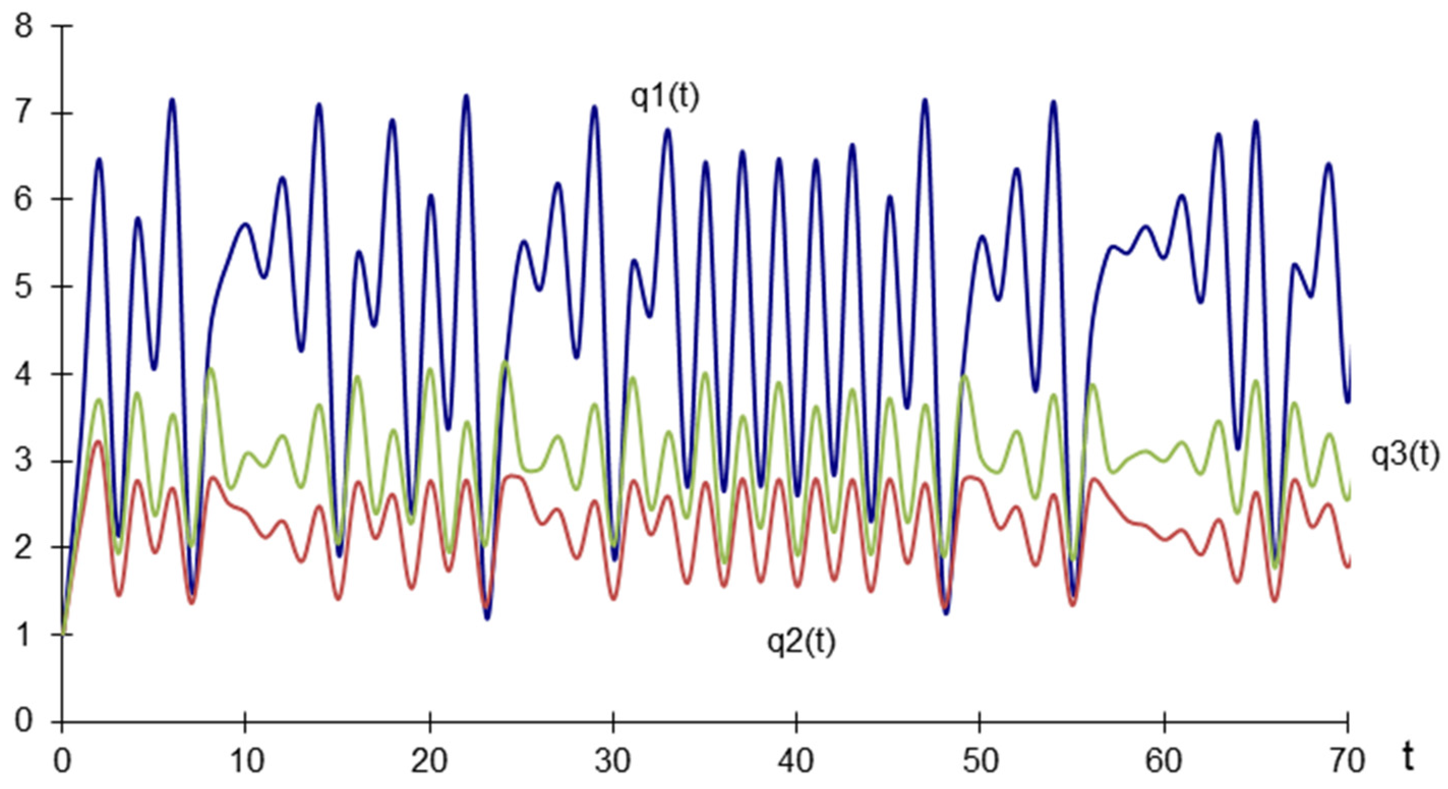
The eigenvalues of this characteristic equation are $\lambda =\left[-1.93;-5.32;0.095\right]$; therefore, the equilibrium quantities are not stable. This situation is illustrated in Figure 3, where the equilibrium quantities do not converge to a stable point.

4. Discussion

In the analyzed model, stable equilibrium quantities could be found under naïve and adaptive expectations. A legitimate question is whether these equilibria remain stable when some exogenous parameters change. This can be analyzed by the maximum Lyapunov exponent [44,45] and the bifurcation diagram [46,47]. To answer this question, the set of data from

Table 1. Exogenous variables.

Company	ARPU $\left({\mathit{\alpha }}_{\mathit{i}}\right)$	Marginal Cost $\left(\mathit{M}{\mathit{C}}_{\mathit{i}}\right)$	Coefficient of Adjustment (μi)
1st company (Orange Slovakia)	15.80	0.166	0.20
2nd company (Slovak Telecom)	12.90	0.177	0.15
3rd company (02)	10.90	0.106	0.20

was further analyzed after changing all exogenous parameters.

After comparing and contrasting the results for the cases of adaptive expectations (corresponding to Figure 2) and naïve expectations (corresponding to Figure 1), we can conclude that in the case of adaptive expectation $q_1>q_2>q_3$, while in the case of naïve expectation $q_1>q_3>q_2$. We can say that under adaptive expectation the two firms in the coalition produce the two highest levels of output, while, under naïve expectation the firm in the coalition with the lower quality produces the lowest output of all three firms, even though its quality is higher than that of the firm that is not in the coalition.

Under naïve expectations, the presented model proved to be stable for any value of $\gamma$ and for the exogenous parameters ${\alpha }_i, M{C}_i$. Matsumoto and Szidarovszky [33] concluded that heterogeneity affects the stability of the positive Cournot equilibrium by shifting the zero-production line as long as it does not affect the stability of the equilibrium quantity. They also concluded that heterogeneity of firms affects the equilibrium point only when the products of the oligopoly are substitutes. Despite the results of these authors and the fact that the products selected for this study are partially substitutable ($\gamma =0.6$), the model is always stable under naïve expectations if the parameters of the model meet the conditions defined in our study.

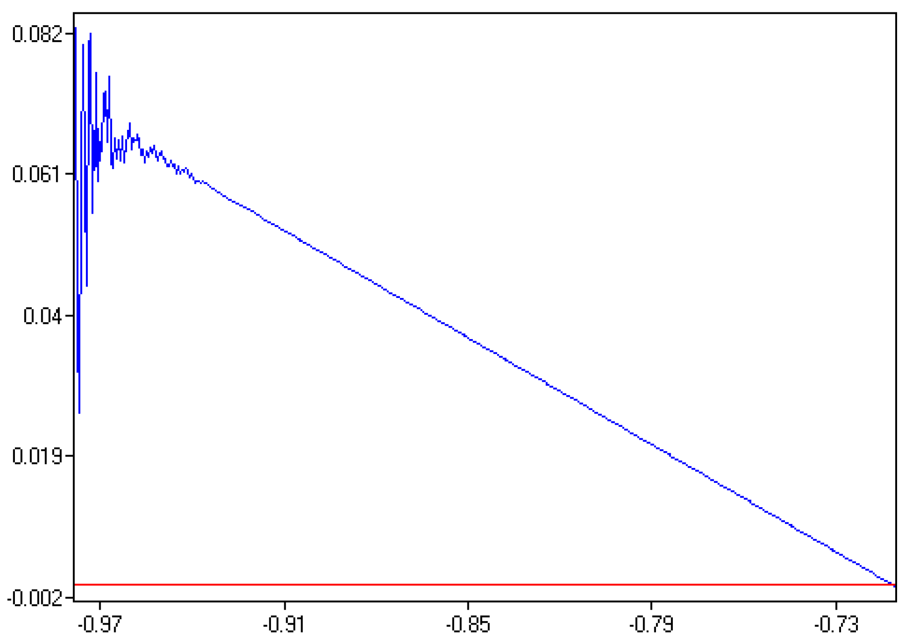
The model with adaptive expectations is stable under all exogenous variables except $\gamma$. In the case presented, oligopoly production substitution was assumed. However, if this assumption is omitted and the products are also defined as complementary, the model with adaptive expectations would be unstable even for $\gamma =\left(-0.978;-0.711\right),$ as shown in Figure 4 with maximum Lyapunov exponent.

.

In the model with real expectations, no stable equilibrium was found, but the quantities oscillated around the points $q_i=\left(5.76; 2.07; 3.13\right)$. Thus, the question arises whether this system could have a chaotic behavior. To illustrate this behavior, the maximum Lyapunov exponent and the bifurcation diagram are shown in Figure 5, where the matching coefficient of the 3rd firm changes along with the change in the quantity of the 1st firm (when ${\mu }_3$ changes).

Figure 5a shows that the maximum Lyapunov exponent for ${\mu }_3$ is sometimes positive in the selected interval. This may indicate the chaotic behavior of the system. Figure 5b shows that the quantity of the 1st firm starts to behave chaotically when ${\mu }_3$ is approximately 0.34.

If we focus only on quantity, without regard to the profit function or stability, the 3rd firm, new to the market, would achieve a higher market share than the 2nd firm $\left(q_3>q_2\right)$, which is part of the coalition, under adaptive and real expectations, resulting in a potential advantage for the 3rd firm under real market conditions.

As mentioned in the previous text, the assumptions of the classical Cournot model can be considered unrealistic under today’s market conditions. Later, several studies have been carried out separately on the differentiation of production [4,24] and on the differentiation of firms [5,6,33,39]. However, studying these phenomena in isolation does not lead to a sufficiently complex representation of reality. Other studies dealt with different types of the firm’s expectations. We can find naïve and adaptive dynamics in [17,35,48,49], and heterogeneous (mixed) expectations of firms, involving real expectations in [50]. The stability of equilibria is very often discussed together with the types of expectations [34,37,51]. Some authors present the cartel extension of the basic Cournot model, the cartelization, or the stability of the cartel equilibrium [28,29,30]. These studies did not consider the coalition against other firms in the market. The research presented in this article does not examine isolated phenomena but combines and integrates them to bring the model closer to reality. The proposed modifications of the basic Cournot model include production differentiation, firm differentiation, coalition strategies, different expectations, and equilibrium stability analysis. Therefore, the results and conclusions of this study contribute to the complex modelling and understanding of oligopolistic firms’ decision making under real market conditions.

5. Conclusions

The subject of this study was an oligopolistic market in which three firms operate in an environment of quantitative competition, the so-called Cournot oligopoly model. The firms and their production were partially differentiated, which brought the theoretical model closer to real market conditions. The main objective was to extend the Cournot duopoly and add another firm, resulting in an oligopolistic market structure assuming partially differentiated production and a coalition strategy between two firms.

This paper presents an oligopolistic model specifically designed for three different types of expectations. It was applied to find and verify the stability of the net equilibrium of oligopolists in the market of telecommunication operators in Slovakia. An indefinite time interval and three types of future expectations were considered: a simple dynamic model with naïve expectations, a model with adaptive expectations and a model with real expectations.

The dynamic system of three companies under naïve expectations proved to be stable, as the eigenvalues of the matrix were less than one and the variables converged to a stable point after approximately 30 time periods. The presented model also proved stable in the case of adaptive expectations, as the quantities converged to a stable point very quickly. In contrast, equilibrium quantities under real expectations were not stable and did not converge to a stable point.

Further analysis proved that the presented model under naïve expectations was stable for any value of $\gamma$ and for the exogenous parameters ${\alpha }_i, M{C}_i$, while the model under adaptive expectations was stable under all exogenous variables except $\gamma$. The model under real expectations was not only unstable, but there was further evidence of the chaotic behavior of the system.

References

- Verhulst, F. Nonlinear Differential Equations and Dynamical Systems; Springer: New York, NY, USA, 1991. [Google Scholar]
- Tišnovský, P. Dynamické systémy v komplexní rovině. Elektrorevue 2001. [Google Scholar]
- Scheinerman, E.R. Invitation to Dynamical Systems; Prentice-Hall: Dover, UK, 1996. [Google Scholar]
- Matsumoto, A.; Szidarovszky, F. Price and Quantity Competition in Dynamic Oligopolies with Product Differentiation. Rev. Investig. Oper. 2011, 32, 204–219. [Google Scholar]
- Singh, N.; Vives, X. Price and Quantity Competition in a Differentiated Duopoly. Rand J. Econ. 1984, 15, 546–554. [Google Scholar] [CrossRef]
- Häckner, J.A. Note on Price and Quantity competition in Differentiated Oligopolies. J. Econ. Theory 2000, 93, 233–239. [Google Scholar] [CrossRef] [Green Version]
- Matsumoto, A.; Szidarovszky, F. Price and Quantity Competition in Differentiated Oligopolies Revisited. DP #138 of Economic Research Institute, 2010. Available online: http://www2.chuo-u.ac.jp/keizaiken/discuss.htm (accessed on 25 January 2014).
- Cournot, A.A. Recherces su les Principes Mathématiques de la Théorie des Richesses; Macmillan: New York, NY, USA, 1838. [Google Scholar]
- Nash, J. Non-Cooperative Games. Ann. Math. 1951, 54, 286–295. [Google Scholar] [CrossRef]
- Friedman, J.W. The legacy of Augustin Cournot. Cah. d´Économie Politique 2000, 37, 31–46. [Google Scholar] [CrossRef]
- Dixon, H.D. Surfing Economics; Palgrave Macmillan: New York, NY, USA, 2001. [Google Scholar]
- Gibbons, R. Game Theory for Applied Economics; Pincenton University Press: Princenton, NJ, USA, 1992. [Google Scholar]
- Selten, R. Eltheoretic Behandlung eines Oligopolmodells mit Nachtragetrgheit. Z. Die Gesamte Staatswiss. 1965, 121, 301–324. [Google Scholar]
- Kreps, D.; Wilson, R. Sequential equilibria. Econometrica 1982, 50, 863. [Google Scholar]
- Milgrom, P.; Roberts, J. Predation, reputation and entry deterrence. J. Econ. Theory 1982, 27, 280–312. [Google Scholar] [CrossRef] [Green Version]
- De Frutos, J.; Gatón, V.; Novo, J. On discrete-time approximations to infinite horizon differential games. arXiv 2021, arXiv:2112.03153. [Google Scholar]
- Kopel, M. Simple and Complex Adjustment dynamics in Cournot Duopoly Models. Chaos Solitons Fractals 1996, 7, 2031–2048. [Google Scholar] [CrossRef]
- Agiza, H.N.; Elsadany, A.A. Nonlinear dynamics in the Cournot duopoly game with heterogenous players. Physical A 2003, 320, 512–524. [Google Scholar] [CrossRef] [Green Version]
- Brock, W.A.; Hommes, C.H. A Rational Route to Randomness. Econometrica 1997, 65, 1059–1095. [Google Scholar] [CrossRef]
- Manski, C.; McFadden, D. Structural Analysis of Discrete Data with Econometric Applications; MIT Press: Cambridge, UK, 1981. [Google Scholar]
- Anderson, S.; de Palma, A.; Thisse, J. Discrete Choice Theory of Product Differentiation; MIT Press: Cambridge, UK, 1993. [Google Scholar]
- Sorger, G. Imperfect Foresight and Chaos: An Example of a Self-Fulfilling Mistake. J. Econ. Behav. Organ. 1998, 33, 363–383. [Google Scholar] [CrossRef]
- Bain, J.S. Relation of Profit Rate to Industry Concentration: American Manufacturing. Q. J. Econ. 1951, 65, 293–324. [Google Scholar] [CrossRef]
- Grisáková, N.; Štetka, P. Equilibrium and Stability in Markets with Differentiated Production; Vysoká Škola Evropských a Regionálních Studií: České Budějovice, Czechia, 2022; p. 157. [Google Scholar]
- Abe, T. Cartel formation in Cournot Competition with Asymmetric Costs: A Partition Function Approach. Game 2021, 12, 14. [Google Scholar] [CrossRef]
- Bimonte, G.; Romano, M.G.; Russolillo, M. Green Innovation and Competition: R&D Incentives in a Circular Economy. Games 2021, 12, 68. [Google Scholar]
- Hagen, A.; von Mouche, P.; Weikard, H.-P. The Two-Stage Game Approach to Coalition Formation: Where We Stand and Ways to Go. Games 2020, 11, 3. [Google Scholar] [CrossRef] [Green Version]
- Kuipers, J.; Olaizola, N.A. A dynamic approach to cartel formation. Game Theory 2008, 37, 397–408. [Google Scholar] [CrossRef] [Green Version]
- CCurranini, S.; Marini, M.A. Sequential play and cartel stability in a Cournot oligopoly. Appl. Math. Sci. 2013, 1, 197–200. [Google Scholar]
- Benchekroun, H.; Xue, L. Cartel Stability in a Dynamic Oligopoly; Centre Interuniversitaire de Recherche en Economie Quantitative: Montreal, QC, Canada, 2005. [Google Scholar]
- Genc, T.S. A dynamic Cournot-Nash game: A representation of a finitely repeated feedback game. Comput. Manag. Sci. 2007, 2, 141–157. [Google Scholar] [CrossRef]
- Forges, F. An approach to communication equilibria. Econometrica 1986, 54, 1375–1385. [Google Scholar] [CrossRef] [Green Version]
- Matsumoto, A.; Szidarovszky, F. Theocharis Problem Reconsidered in Differentiated Oligopoly. Econ. Res. Int. 2014, 2014, 630351. [Google Scholar] [CrossRef] [Green Version]
- Theocharis, R.D. On the stability of the Cournot solution on the oligopoly problem. Rev. Econ. Stud. 1960, 27, 133–134. [Google Scholar] [CrossRef]
- Bischi, G.I.; Kopel, M. Equilibrium selection in a nonlinear duopoly game with adaptive expectations. J. Econ. Behav. Organ. 2001, 46, 73–100. [Google Scholar] [CrossRef] [Green Version]
- Fisher, F.M. The stability of the Cournot oligopoly solution: The effects of speeds of adjustment and increasig marginal costs. Rev. Econ. Stud. 1961, 28, 125–135. [Google Scholar] [CrossRef]
- Szidarovszky, F.; Yen, J. Stability of a special oligopoly market. Pure Math. Appl. 1991, 2, 93–100. [Google Scholar]
- Bischi, G.I.; Galletgatti, M.; Naimazada, A.A. Symmetry-breaking bifurcations and representative firm in dynamic duopoly games. Ann. Oper. Res. 1999, 89, 253–272. [Google Scholar] [CrossRef]
- Elabbasy, E.M.; Agiza, H.N.; Elsadany, A.A.; El-Metwaly, H. The dynamics of Triopoly Game with Heterogeneous Players. Int. J. Nonlinear Sci. 2007, 3, 83–90. [Google Scholar]
- Slovak Telecom, “www.telecom.sk”, 2013. Available online: https://www.telekom.sk/documents/10179/44166/Slovak+Telekom+Ro%C4%8Dn%C3%A1+spr%C3%A1va+2013.pdf/3129b031-d165-4924-9ad9-5ed7bcabc204 (accessed on 13 October 2022).
- Telefónica Slovakia, “www.spolocnost.o2.sk”, 2013. Available online: https://spolocnost.o2.sk/media/3/vyrocna-sprava-2013.pdf (accessed on 13 October 2022).
- Orange, “www.finstat.sk”, 2013. [Online]. Available online: https://finstat.sk/35697270/zavierka (accessed on 13 October 2022).
- Arrowsmith, D.K.; Place, C.M. Dynamical Systems: Differential Equations, Maps and Chaotic Behaviour; Chapman & Hall/CRC: London, UK, 1998. [Google Scholar]
- Strogatz, S.H. Nonlinear Dynamics and Chaos: With Applications to Physics, Biology, Chemistry and Engineering; Addison-Wesley: New York, NY, USA, 1994. [Google Scholar]
- Dingwell, J.B. Wiley Encyclopedia of Biomedical Engineering; Wiley: New York, NY, USA, 2006. [Google Scholar]
- Blanchard, P.; Devaney, R.L.; Hall, G.R. Differential Equations; Thompson: London, UK, 2006. [Google Scholar]
- Kellert, S.H. The Wake of Chaos: Unpredictable Order in Dynamical Systems; University of Chicago Press: Chicago, IL, USA, 1993. [Google Scholar]
- Huang, W. Theory of Adaptive Adjustment. Discret. Dyn. Nat. Soc. 2001, 5, 247–263. [Google Scholar] [CrossRef] [Green Version]
- Szidarovszky, F.; Okuguchi, K. Alinear oligopoly model with adaptive expectations: Stability reconsidered. J. Econ. 1988, 48, 79–82. [Google Scholar] [CrossRef]
- Kirman, A.; Zimmermann, J.-B. Economics with Heterogeneous Interacting Agents, Lecture Notes in Economics and Mathematical Systems; Springer: Berlin/Heidelberg, Germany, 2001. [Google Scholar]
- Agiza, H.N.; Bischi, G.I.; Kopel, M. Multistability in a Dynamic Cournot Game with Three Oligopolists. Math. Comput. Simul. 1999, 51, 63–90. [Google Scholar] [CrossRef]
Figure 1.
Equilibrium quantities for naive expectations—dynamic map.
Figure 2.
Equilibrium quantities for adaptive expectations—dynamic map.
Figure 3.
Equilibrium quantities for real expectations—dynamic map.
Figure 4.
Maximum Lyapunov exponent for adaptive expectations and .
Figure 5.
Adjustment coefficient changing: (a) maximum Lyapunov exponent for ; (b) bifurcation diagram for quantity of the 1st firm when .