
Price Competition with Differentiated Products on a Two-Dimensional Plane: The Impact of Partial Cartel on Firms’ Profits and Behavior

1
FactSet Research Systems Inc., 43 Glover Ave. Fl. 7, Norwalk, CT 06850, USA
2
Management Board of the Center for Analyzes and Risk Management, New Bulgarian University, ul. “Montevideo” 21, g.k. Ovcha Kupel 2, 1618 Sofia, Bulgaria
*
Author to whom correspondence should be addressed.
Games 2023, 14(2), 24; https://doi.org/10.3390/g14020024
Submission received: 31 December 2022
/
Revised: 6 March 2023
/
Accepted: 12 March 2023
/
Published: 15 March 2023
Abstract
:A numerical procedure capable of obtaining the equilibrium states of oligopoly markets under several assumptions is presented. Horizontal and vertical product differentiation were included by taking into account Euclidean distance in a two-dimensional space and quality characteristics of the product. Different quality preferences of consumers were included in the model. Firms implement two strategies in the market: profit maximization and market share maximization. Numerical discretization of a two-dimensional area was performed for computing the equilibrium prices which allows one to consider any market area and any location of the firms. Four scenarios of oligopoly markets were developed by combining both strategies from one side and competitive behavior and a partial cartel agreement from another side. The main differences between the scenarios are outlined. Profits, market shares and equilibrium prices are presented and compared. The influence of collusion, the existence of participants with a market share maximization strategy and consumer preferences on the firm’s profits and equilibrium prices were examined. Cases whereby firms prefer to leave the cartel were investigated. Best locations for the setting of a new store for profit maximization are shown and discussed.
1. Introduction
Strategic interactions in oligopoly markets have been investigated since the nineteenth century. At that time, Cournot [1] and Bertrand [2] developed their famous competitive oligopoly models. Cournot developed an oligopoly model with two firms that compete by simultaneously setting their output quantity. Cournot’s model was highly abstract at that time, and Bertrand criticized Cournot’s assumption as “unrealistic” because of the quantity competition hypothesis. Bertrand developed an oligopoly model wherein firms compete by simultaneously setting their price. The equilibrium prices of both models represent a Nash equilibrium in oligopoly games. The Nash equilibrium is achieved under the assumption that each firm tries to achieve its optimal targets, i.e., profit maximization. Once the equilibrium is reached, the market participants cannot further improve their profits, and any modification of their quantity or price will result in a reduced profit [3]. Quantity (Cournot) versus price (Bertrand) competition has drawn great attention in the literature, and many researchers have compared the models, considering different assumptions [4,5,6,7].
Product differentiation represents an important component of economic models. Perfectly homogeneous products and perfectly informed consumers would lead to Nash equilibriums with equal prices for each firm. Differentiated products, however, introduce consumer preferences and generally lead to equilibriums with different prices. There are two basic types of product differentiation—horizontal and vertical [8]. In horizontal product differentiation, if the prices are equal, some consumers will buy one product and others will buy another. The choice depends on the consumers’ preferences. Color and distance are examples of horizontal product differentiation. In vertical product differentiation, if the prices are equal, all consumers will prefer one of the products. Quality is an example of vertical product differentiation. Multi-characteristic product differentiation represents products that differ in more than one characteristic.
The simplest way to consider horizontally differentiated products that differ by distance is to use Hotelling’s linear city model, introduced by Hotelling [9]. In this model, the competition arises along a single linear street. Another way to achieve this that is popular in the literature is the application of a circular city model where the competitors are located around a circle and each firm competes with its closest neighbors, as presented by Salop [10].
Both models are useful for investigating the general properties of horizontally differentiated products and their influence on equilibrium prices and market share; however, one-dimensional models distort the nature of spatial competition. Some of the limitations include the fact that each firm (or store) in a one-dimensional model cannot have more than two spatial competitors, or the effect of boundedness can be represented only by two firms located at the ends. Two-dimensional models overcome these restrictions and give the opportunity to model the real locations of firms. An extension of Hotelling’s duopoly model was developed by Economides [11], where a two-dimensional plane was considered instead of linear or circular city models. The author considered only two competitive firms and used a utility function that is linear in Euclidean distance. The boundary between market areas of the firms was found analytically as hyperbola. Okabe and Aoyagi [12] analyzed the equilibrium of competitive firms in an infinite two-dimensional space. Linear utility function and inelastic demand were used and the market areas of the firms were obtained analytically by Voronoi polygons.
An important class of problems that involve distance as horizontal product differentiation fall into the so-called spatial competition defined by Losch [13], i.e., competition where firms set their locations. Brown-Kruse at al. [14] studied spatial competition between two firms on a linear market. The authors presented theoretical and experimental results depending on the location choice. Cahan at al. [15] considered a two-dimensional space competition where firms compete by location, and introduced a probability vector that assigns to the consumers a probability that they will buy from firms other than the nearest one. The authors showed that Nash equilibrium exists in the central region of the marked bounded by hyperbolas computed analytically. More information on spatial competition can be found, for example, in [16,17,18,19,20].
The influence of product differentiation on equilibrium prices and firms’ profits has been investigated by many scientists in the past few decades. It was concluded in several works that an increase in product variety leads to gains for the competitive firms [21,22]. Li and Ji [23] developed a duopoly model with differentiated products where one of the firms invests in cost-reducing innovation and licenses its technology. Under the influence of innovation and licensing, the Cournot competition resulted in lower industry profits, greater consumer surplus and greater social welfare. An equilibrium solution was found analytically by first-order conditions. Lahmandi-Ayed [24] developed a price competition model with horizontally differentiated products by using Hotelling’s linear city model. The author refuted the conventional understanding that the equilibrium prices increase with the consumer’s income, and proved the opposite. He assumed that, due to low incomes (or high transportation cost), the market may remain uncovered as only consumers located near the stores would buy the product, therefore leading to de facto local monopolies. An increase in income (or decrease in transportation cost) will cover the market and create competition between the firms which in turn will lead to a price reduction. Askar and Al-khedhairi [25] studied the Bertrand duopoly model, where firms have incomplete information and compete via the maximization of relative profits. The authors investigated the equilibrium stability due to the variable degree of horizontal differentiation and the variable parameter of the cost function. Kishihara and Matsubayashi [26] studied the conditions and benefits of repositioning firms’ locations and updating their prices in a duopoly with horizontally differentiated products by adopting Hotelling’s linear city model. Liu et al. [27] developed a two-stage game where firms make a decision regarding whether to invest to differentiate their products horizontally by considering the duopoly game and strategies based on Cournot and Bertrand competitions. Brady [28] used asymmetric horizontal differentiation in a Cournot duopoly including advertising in the demand function, which also increases the level of differentiation.
Antitrust policy protects competition, thus benefiting consumers with lower prices and better products. It requires that competitive firms in a market do not discuss their prices with each other. Otherwise, they might engage in cartel agreements that are illegal in most jurisdictions. The firms entering into such agreements aim at increasing their profits by collaborating at the detriment of a free competitive market. Most often, cartels arise in markets with few participants and homogeneous products.
Garrod and Olczak [29] outlined the differences between tacit and explicit collusion. They found that tacit collusion, rather than explicit, is more likely to appear in markets with few symmetric firms. Furthermore, explicit collusion becomes more likely to appear as the number of symmetric firms increases. Fonseca and Normann [30] investigated the difference between explicit and tacit collusion. They confirmed that communication helps to obtain higher profits and that collusion is easier with fewer firms on the market.
Kuipers and Olaizola [31] analyzed cartel formation from a dynamic perspective. They presented a dynamic model for cartel formation where the authors allow the cartel to change over time, i.e., firms can leave or enter the cartel if they obtain benefits from this action. The effect of price agreements among firms on their product variability was investigated by Gabszewicz et al. [32]. The authors ascertained that, under a cartel agreement, it is more profitable for the companies to withdraw some products from the market and to reduce competition. Profits were expressed as quadratic function of price and equilibrium was found by first-order conditions. Correani and Dio [33] examined the formation of links in oligopolies with horizontally and vertically differentiated products. They defined the links between two firms in terms of a reduction in their marginal costs based on knowledge sharing. They concluded that firms might form collaborations if they offer products with low vertical differentiation and high horizontal differentiation. Bos and Marini [34] studied cartel stability in a market with vertically differentiated products. They showed that the supplier with the lowest noncooperative price–cost margin is most inclined to leave the cartel. Song and Wang [35] analyzed the collusion stability in a Cournot competition with differentiated products with network externalities. They found that collusion becomes more sustainable for closer substitutes of products. Biancini and Ettinger [36] investigated the effect of vertical mergers on competition and showed that vertical integration favors the development of collusion. Grisáková at al. [37] considered the Cournot oligopoly model with three firms, where two of them form a cartel. The authors showed that under real expectations, i.e., firms do not have complete information about the market demand function, there is no stable equilibrium and there are cases in which chaotic behavior might be observed.
While a profit maximization strategy seems a natural choice for any participant in the market, it has been shown in a multitude of works that a market share maximization strategy also leads to an increase in profitability [38,39]. There exist a variety of strategies that lead to an increase in market share, and a few of them are outlined here. Porter [40] proposed a cost leadership strategy that aims at reducing costs throughout the value chain and offering a product with acceptable quality in order to maximize the market share. Ward at al. [41] proposed the development of new products to increase the market share. The strategy is known as the broad differentiator and its aim is to offer a wide range of products in various markets. Venkatraman [42] defined “aggressiveness” as a strategy for increasing market shares. It is based on allocating resources, such as pursuing faster product innovation or market development than competitors. Mintzberg [43] proposed a typology of generic strategies, including price differentiation. He linked this strategy with Porter’s cost leadership.
The equilibriums solutions of these models were obtained analytically by using first-order optimality conditions. In some works, such as in [35], authors used second-order condition to guarantee that the obtained solution is maximization of the profit. While majority of the works derive analytical solutions, there are cases in which the equilibrium solution requires numerical computations. Jiang at al. [44] analyzed two-stage non-cooperative multi-agent Cournot game under uncertainties. The equilibrium conditions were converted into two-stage stochastic variational inequality which were solved by smoothing technique and application of Newton’s method. A non-smooth Newton method was used in [45] to solve variational inequality problem which represents the equilibrium of an oligopolistic market with non-cooperative firms who share a certain amount of rare resource. In [46] authors study the dynamics of Bertrand oligopoly under randomly fluctuating demands. They represented the equilibrium as nonzero-sum stochastic differential game which is characterized by a system of nonlinear partial differential equations. The system is solved numerically by finite difference methods. Numerical methods were also used for simulating the dynamical behavior of Cournot/Bertrand games and for further bifurcation analysis [47,48,49].
The goal of the current work was to combine the aforementioned common cases in oligopolistic markets into a modeling framework and to develop a numerical procedure that is able to compute equilibrium prices. The model includes vertical product differentiation in two-dimensional space, competition among firms with (or without) partial cartel, and maximization of profits and/or maximization of quantity strategies. Furthermore, the model is able to handle any area of interest and any locations of the participants, as well as, complex expressions of consumers’ utility functions, including nonlinearities. These requirements, in combination with two-dimensional space competition, impose the usage of numerical techniques for computing the equilibrium solution. The proposed numerical approach consists of two components: numerical discretization of the market area and numerical solution of the optimization problem.
The optimization problem is solved by modification of the gradient ascent method [50] with an adaptive step size [51]. The method needs an expression for the demand function that depends on the market share of each participant. The market share is obtained by discretization of the whole area into smaller elements and assigning to each element a particular market share depending on a utility function. The convergence of the numerical procedure with the discretization element size and with the iterative steps of the gradient ascent method is presented.
Distance in two-dimensional space is used to represent horizontal differentiation and Voronoi diagrams [52] are used to represent the market share of each firm. The quality of the product is used for vertical differentiation. Consumers select the best store via a utility function that is expressed as function of distance, price, product quality and quality preferences of consumers. First, the competitive scenarios are examined, where either all firms are assumed to set their prices to maximize their profits or some firms are assumed to be market share maximizers. Then, a group of firms are allowed to form a cartel and jointly maximize their profits. These different scenarios are compared and analyzed.
It is shown that a participant with a market-share-maximizing strategy significantly disrupts the cartel’s profit. Its disruption of the cartel’s profit is much greater than its disruption of firms’ profits in a competitive market. As a consequence, some of the firms forming the cartel will prefer to leave it and achieve higher profits by reducing their prices and increasing their market share. These firms will capture their market share not only from the participants following a market share maximization strategy but also from the cartel members, which in turn would also prefer to leave the cartel.
The best locations for the setting of a new store in a market with a partial cartel are investigated. The firms would prefer to select new store locations in such a way as not to disrupt the cartel and use its higher prices as an “umbrella”. This strategy leads to higher profits than when disrupting the cartel and achieving a larger market share.
The possibility of the model to combine two types of strategic behavior, to consider consumers with different quality preferences and its applicability to markets on two-dimensional space by any shape, allows one to analyze variety of real markets and to develop microeconomic strategies for oligopolistic markets. Furthermore, the generality of the model to consider partial cartels between any combination of companies provides basis for further developments of cartel detection algorithms.
The paper is organized in the following way. The optimization problems are derived in Section 2. The utility function, which takes into account the different product characteristics and consumer preferences, is described in Section 3. Section 4 provides details about the demand function. Section 5 presents the numerical procedure used to obtain Nash equilibriums and capable of handling the two-dimensional location of consumers and stores. Finally, in Section 6, we present and analyze the equilibrium states of oligopoly markets under competitive behavior and under the existence of a cartel. The main differences are outlined, and the profits of each participant, market share and equilibrium prices are presented and compared. Cases are shown wherein some cartel members are willing to leave and gain higher profits. At the end of the section, we show the best locations for the setting of a new store with a profit maximization strategy.
2. Mathematical Model
The model assumes that there are firms on the market denoted by , . Each firm may have several stores. Prices at different stores of one firm may differ. Prices of firm are denoted by , where the superscript denotes the store.
The profit of each firm is obtained as the difference between the total revenue and total cost from all stores of the firm. The profit function of firm is expressed in the following way:
where
- represents the sold quantity of the product by firm at store ; it is the demand generated by the consumers;
- represents the price of the product offered by firm at store ;
- represents the marginal cost of the product for firm related to store ;
- represents a fixed cost for firm at store , i.e., expenses that do not depend on the sold quantity.
It is shown in Section 4 that the demand function depends not only on the prices determined by the firms, but also on the locations of all stores, the density of consumers, the quality of products and the quality preferences of consumers. These components, with the exception of the prices, do not change during the establishment of Nash equilibrium. Thus, the demand function of each store is written as dependable only on the prices determined by the firms:
The demand function of each firm is obtained as the sum of the demand functions of all stores:
The profit of each firm also depends on the prices of all firms:
The firms determine the prices of their stores in order to realize their strategy, profit maximization or market share maximization. The prices are not allowed to be negative and the profits in a market share maximization strategy are also not allowed to become negative. The consumers have equal demands for the product and the market is assumed to be covered.
This section continues by presenting the four scenarios mentioned in the Introduction as optimization problems. The Nash equilibrium represents the solution of the optimization problem. Each scenario requires an evaluation of the demand Function (2). The process of estimating the demand function is presented in Section 4. It requires a utility function, which is derived in Section 3.
2.1. Scenario 1
Scenario 1 represents a competitive market with a profit maximization strategy. In this scenario, each firm attempts to maximize its own profit by selecting the best prices for its stores, i.e., firm selects prices , which maximize the profit function .
The Nash equilibrium is obtained by solving the following optimization problem:
2.2. Scenario 2
This scenario assumes that some of the firms are in a cartel agreement, while the rest of the firms determine their prices independently. The cartel is modeled by considering that its members have agreed a common price for the product. The price of the cartel is set to maximize the collective profits of the participants in the cartel. The expected result of such an agreement is that the firms in the cartel will achieve higher profits than when determining their optimal prices independently.
Let us assume that firms are in the cartel, while firms determine their prices independently. The common price of the cartel is denoted by and the prices of the other participants on the market are denoted, as before, by , for . The Nash equilibrium is obtained as the solution of the following optimization problem:
where represents the common profit of the participants from the cartel, i.e., is expressed as
2.3. Scenario 3
Scenario 3 represents a combination of both strategies and considers that all firms determine their prices independently. Some of the firms determine their prices in order to maximize their profits. The rest of the firms determine their prices to maximize their market share.
Let us assume that firms attempt to maximize their profits and firms attempt to maximize their market share. A constraint is added to the optimization problem, implying that the profit of the firms that maximize their market share must be non-negative. The optimization problem that leads to the Nash equilibrium of this scenario is written in the following way:
2.4. Scenario 4
This scenario considers both strategies and assumes that some of the firms are in a cartel agreement while the other firms determine their prices independently. The firms in the cartel attempt to set a common price that maximizes their common profit. Some of the independent firms maximize their profits, while the other independent firms maximize their market share.
Let us assume that the firms are in a cartel agreement with a common price denoted by . The firms determine their prices independently and they attempt to achieve maximal profits. The rest of the firms, , also determine their prices independently, but they attempt to maximize their market share. The Nash equilibrium is obtained by solving the following optimization problem with constraints:
3. Utility Function for Horizontal and Vertical Product Differentiation
The product offered by the firms in the model is assumed to differ in terms of two characteristics—location and quality. The location introduces a horizontal differentiation and the quality introduces a vertical differentiation of the product. Each consumer chooses the store depending on the price of the product, the distance between the store and the consumer and the quality of the product. If two stores offer products with the same quality and the same price, the consumer will prefer the closest one. If two stores offer products with the same price and they are located at an equal distance from the consumer, the consumer will prefer the store offering the higher-quality product. The consumer chooses the store that maximizes the utility function defined in this section.
In reality, consumers do not have identical behavior and differ in terms of a variety of characteristics, including their different preferences for quality. For example, some consumers are indifferent to the product quality and prefer to buy the product from the cheapest store, while other consumers have strong quality preferences and would prefer to pay a higher price, even if they have to travel a greater distance.
In order to include the variety of consumers’ preferences for quality, different values for the strength of preferences, denoted by , , are introduced in the utility function. Each quality preference relates to a particular part of the consumer population, denoted by the subscript . It is assumed that varies between zero and one. If is zero, then the consumer is indifferent to the quality of the product and would choose the product based on its price and distance only. Higher values of imply stronger quality preferences of the consumers.
The utility function describes the benefit of a consumer buying a product from particular firm and store. The utility function depends on the distance between consumer’s location and location of the store, the price of the product at that store, its quality and quality preferences of the consumer. The utility function for a consumer that belongs to type and is located at position applied to store of the firm is denoted by . The following expression is used for the utility function
represents the price, the distance between the consumer and the store is computed as Euclidean distance and it is denoted by , denotes consumer’s preferences on quality, as defined above, and represents the quality of the product offered by firm .
The coefficients , and are assumed to be constants. Their values should be determined based on the application of the analysis.
The first term can represent the average number of products that consumers buy for the period under analysis. This number is represented by . The coefficient can also be used as weight in the utility function that controls the importance of price in comparison to the other arguments.
The second term in the utility function, , relates the distance to the store and the price of the product. As an example, one might consider the price of the fuel at gas stations. Traveling the distance generates expenses for the consumer by the cost of the fuel. In this case, the coefficient can be determined so that the term represents the cost that a consumer pays to travel the distance .
The coefficient is used to increase or decrease the importance of consumers’ quality preferences in relation to the price and distance. The coefficient is included in the utility function in order to ensure that can be limited between zero and one and, at the same time, to allow us to model the importance of quality preferences in relation to the other two factors: price and distance.
4. Estimation of Demand Function
Both strategies considered in this work require knowledge of the demand function. The demand function of each participant is determined by the prices of all firms, as stated in Equation (2), and the utility function.
The demand function needs to be estimated separately for each consumer type. Furthermore, each store will have different consumer areas, depending on consumers’ quality preferences. The consumer area of a store for a specific consumer type represents the area in which all consumers of this type would prefer to buy the product from that store.
Let denote the whole region under analysis, i.e., represents the region where all stores and all consumers are located. denotes the region representing the consumer area of store of firm for consumers of type . It is determined in the following way:
where represents the utility function for a consumer located at position with a quality preference of type applied to store of firm , as defined in Equation (10).
It is assumed that consumers are continuously distributed along area . Let represent the density of type consumers. The demand function of firm and store for consumers of type , is given by
The demand function of each store is obtained by the sum of the demand functions of all consumer types:
where represents the total number of consumer types.
It is important to note that the demand function does not depend only on consumer type. The demand function defined in Equation (12) shows that it is determined by consumer’s area and consumer’s density. The consumer’s area is determined by the utility function, which depends not only on consumer’s type, but also on price, distance and quality. Hence, the demand function also depends on price, distance and quality.
The demand function derived in Equation (13) is used to compute the profits defined in Equation (1). The demand function that represents the overall market share of the firm is defined in Equation (3). This expression of the demand function is attempted to be maximized in Scenarios 3 and 4.
5. Numerical Solution and Convergence Study
5.1. Discretization of Two-Dimensional Plane
The solution of the derived optimization problems requires knowledge of the demand function for each firm by a given vector of prices. The demand function involves the determination of the consumer area of each firm, which depends on the utility function. For a given location of a consumer—for example, —one needs to compare all the utility functions defined for the consumer’s location and each store and assign the store to the location and, respectively, the firm that derives the highest utility. In this way, the area under analysis is divided among all firms, and each firm has its own consumers located in the area assigned to the firm. Once the consumer areas of each firm are known, the demand functions are obtained by taking into account the consumer area and consumers’ density, as shown in Section 4.
The computation of the firm’s consumer areas represents a Voronoi partition with the distance function defined by the utility function presented in Section 3. There are a variety of algorithms for the construction of Voronoi diagrams [52] with distance functions, such as Euclidean distance, Manhattan distance or other simple distance functions. The utility function defined in Section 3 involves not only the Euclidean distance between the consumers and the firm’s stores, but also the price, quality and consumer’s preferences for quality. The utility function complexity requires a numerical procedure to decompose the plane into Voronoi cells that represent the consumer area of each firm.
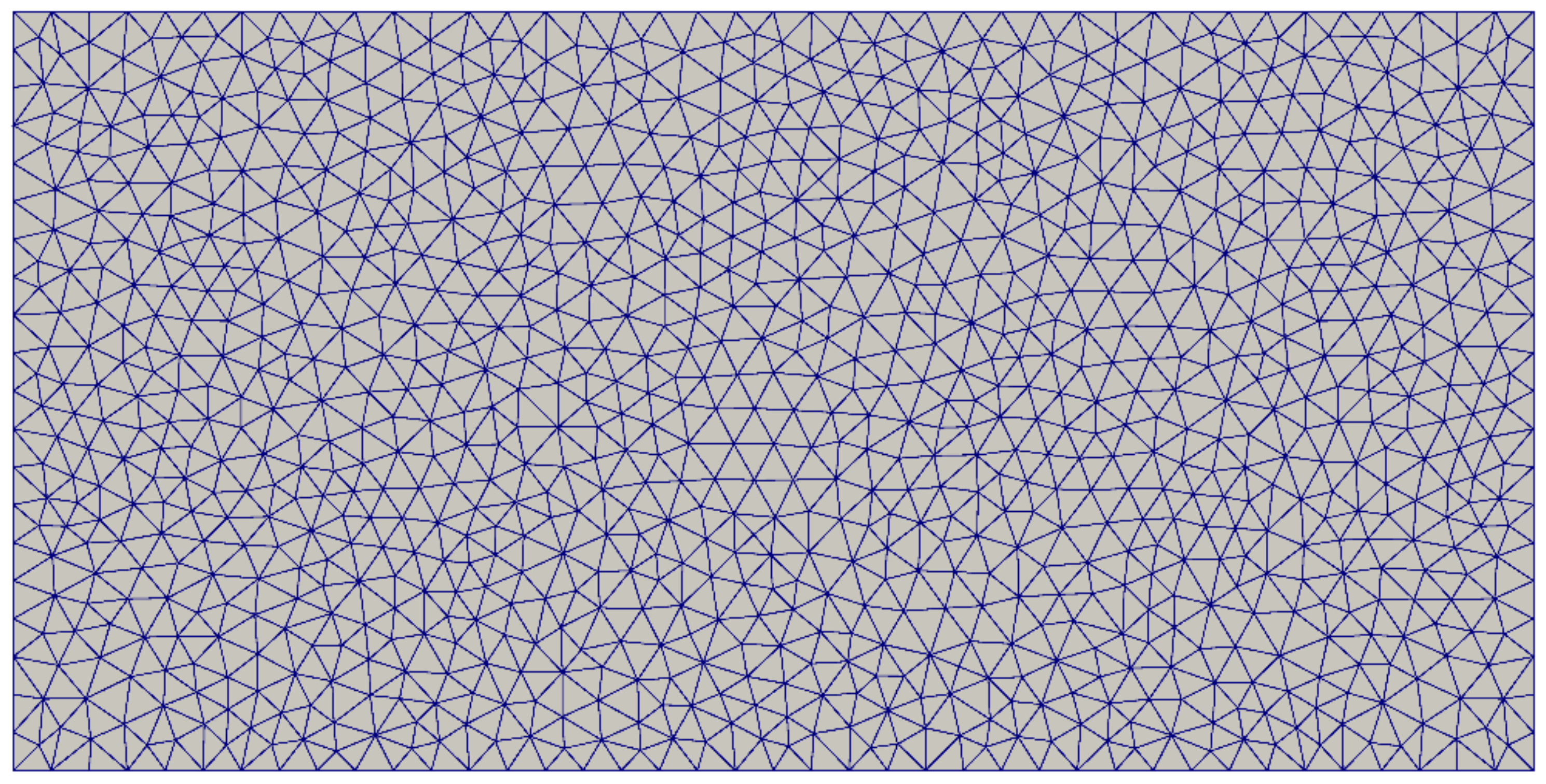
The numerical determination of Voronoi cells with regard to the utility function is performed by dividing the total area into small triangles. It is assumed that each triangle belongs to the consumer area of a single store. The consumer area of each triangle is determined by the utility function applied to the center point of the triangle. The accuracy of the results is improved by reducing the size of the triangles and increasing their number. Gmsh software [53] is used to generate a mesh of triangles. An example of such a division of the total area into small triangles is presented in Figure 1.
5.2. Iterative Procedure for Nash Equilibrium Solutions
The derived optimization problems represent multi-objective optimization problems [54], which are solved by modifying the gradient ascent method [50]. The numerical procedure is illustrated for Scenario 1; it is assumed that the firms have a single store and the superscript index denoting the store number is omitted for simplicity. Scenario 1 represents an optimization problem of objective functions, each of them depending on variables, , while the maximization of each objective function is sought by modifying only one of the variables. This condition comes from the assumptions accepted in oligopoly markets with a Nash equilibrium: each participant on the market selects only its own price in order to achieve its goal. For example, firm 1 attempts to maximize its own profit by selecting the best price of its own product to this end. Thus, the numerical procedure aims for the iterative computation of the vector of prices, where each price follows the increasing direction of the profit function with respect to that price only. Hence, a gradient ascent method is applied to each objective function by adding a scaled value of its derivative with respect to the price, by which the maximization of the objective function is sought. In addition, a Barzilai–Borwein [51] adaptive step size is used for better performance and a higher rate of convergence.
Other popular optimization approaches of multi-objective optimization problems, such as the conversion to a single-objective optimization problem, would try to maximize one objective function that involves all profits. This obviously contradicts the presented scenarios of oligopoly markets and thus it is not applicable in these cases.
The price vector , which represents the Nash equilibrium state, is obtained iteratively by modifying each element of the vector in the following way:
where the superscript denotes the iteration number. is the adaptive step size obtained by the application of the Barzilai–Borwein method. is set to 0.1, while the other adaptive values are defined in Equation (15).
Although the Barzilai–Borwein adaptive step size was developed and used for gradient descent/ascent methods, it is shown numerically that the adaptive step size performs well for the current optimization problem and significantly increases the convergence rate. The adaptive step size is defined by
where denotes the dot product of two vectors; represents the vector of prices and is defined to be
where
The iterative procedure requires the computation of the derivative of the demand function of firm , denoted by , with respect to the price of the same firm, i.e., . A central difference formula is used for this purpose:
where is a sufficiently small constant. Because of the discretization of the two-dimensional plane, the demand functions become non-smooth functions of prices ; thus, the selection of an appropriate value of , together with the selection of an appropriate mesh, is critical for the convergence of the iterative method.
The optimization problems are nonlinear optimization problems. The numerical procedure depends on the initial point of the iterative method and the optimization problems might have more than one solution. In order to have consistent results for all scenarios that are comparable, the same initial points are used for the iterative procedure for each scenario. In the current work, the vector of marginal costs is used as an initial point.
5.3. Convergence Study
The rate of convergence of the solution with respect to the mesh size and the number of iterations in the modified gradient ascent method are analyzed in this sub-section. The convergence study was performed on Scenario 1 with eight participants located in a rectangular area. The product quality and consumer preferences were not considered in the convergence analysis. More details about the dimensions of the rectangle and the locations of the participants are given in the next section, where the results are discussed.
Five different meshes were used; the first one is presented in Figure 1. Each subsequent mesh was generated from the previous one by reducing each triangle into four smaller ones—hence, decreasing the size of the element by two. The generated number of elements for each mesh with the average size of the elements is shown in Table 1. The absolute error of the norm of the vector of prices and the convergence of the prices of two firms are shown in Figure 2. A quadratic rate of convergence was observed in the numerical experiments.
The comparison of the convergence rate between a Barzilai–Borwein adaptive step and a constant step, as well as the convergence rate of the iterative method by using different meshes, is shown in Figure 3. The rate of convergence of the Barzilai–Borwein method significantly exceeds the usage of a constant step. One can see that the usage of a larger constant step with a coarse mesh forces the iterative algorithm to oscillate around the solution (Figure 3a), or . These oscillations result from the non-smooth demand function, which leads to jumps in the computation of its derivative with respect to price. The smoothness of the demand function was improved by refining the mesh (Figure 3b).
The convergence rate becomes slower when vertically differentiated products were introduced. A comparison of the convergence rate with the iterative steps, considering different values for quality of the product for some of the firms, is shown in Figure 4. Bigger differences of quality led to a lower rate of convergence.
Finally, the consumer areas’ convergence with mesh refinement is shown in Figure 5. One can see that, for coarse meshes, small changes in price can lead to jumps in the consumer area and consequently to jumps in the demand function. As the mesh becomes finer, the demand function becomes smoother.
6. Results
A rectangular area was considered for the numerical results. The dimensions of the rectangle were set to be 80 × 40 km. Eight firms, denoted by numbers from 1 to 8, were assumed to compete under four scenarios.
The four different scenarios given in Section 2 are represented here again by assigning a particular strategy to each of the eight firms:
Scenario 1—All firms are independent and determine their prices in order to maximize their profits.
Scenario 2—Firms 1 to 6 are in a cartel agreement, while firms 7 and 8 are independent. The cartel and the independent firms determine their prices by maximizing their profits.
Scenario 3—All firms are independent. Firms 1 to 7 determine their prices in order to achieve the maximum profit, while firm 8 determines its price to maximize its output (i.e., market share).
Scenario 4—Firms 1 to 6 are in a cartel agreement, while firms 7 and 8 are independent. The cartel and firm 7 determine their prices by maximizing their profits; firm 8 determines its price in order to achieve the maximum output.
For Scenarios 1 and 2, the marginal cost of all firms was set to be equal, . For Scenarios 3 and 4, where firm 8 attempts to maximize its market share, the marginal cost of firm 8 was set to be , in order to allow profits of 0.02 per unit product. The rest of the firms from Scenarios 3 and 4 had a marginal cost of 1.82.
It is shown in [55] that cartel members prefer to sell higher quality product. Thus, the firms that participate in the cartel in Scenarios 2 and 4 are assumed to offer a product of higher quality than the other firms. Furthermore, the firms that form the cartel are considered to offer product with the same quality, since lower quality firm in the cartel has the strongest incentive to leave it [34]. These statements are confirmed by the current numerical approach. Figure 6 shows the profit of the cartel from Scenario 2 as function of the quality of the product, considering that firms 7 and 8 offer product with quality . A fixed cost proportional to the quality of the product is used with value . One can see that the cartel achieves the highest profit when it offers the product with quality . It was also confirmed by numerical experiments, that if a firm from the cartel offers the product with different quality, then either the firm or the cartel would benefit more if the firm is not part of the cartel. Thus, in the numerical simulations it is assumed that , for and for .
Sensitivity analysis measures the impact of one or more variables to the solution of the numerical model. A sensitivity analysis of parameters , and , considering Scenario 1, is shown in Figure 7. The results show that the model is robust to changes of these parameters. The following values were used: , , in the numerical simulations.
The quality preferences used for the present analysis and the percentage of the population that belong to each quality preference type are presented in Table 2. According to the table, 10% of the consumers are indifferent to the quality of the product (Type 1), 10% of the consumers have strong quality preferences (Type 5) and the rest of the consumers are between these two cases. The density of consumers is uniformly distributed along the whole area.
6.1. Comparison of Scenarios
Eight firms, each with one store, were assumed in all scenarios. The rectangle was divided into eight equal squares and the stores were located in the middle of the squares. The position of each store is presented in Figure 8. Even though the numerical procedure allows any location of the firms, this type of symmetrical location was preferred in the numerical experiments because it permits a better interpretation of the results and a clear distinction between the different scenarios. Non-equidistantly located firms are analyzed in Section 6.3. Mesh 4, shown in Table 1, was used for the numerical results in all scenarios.
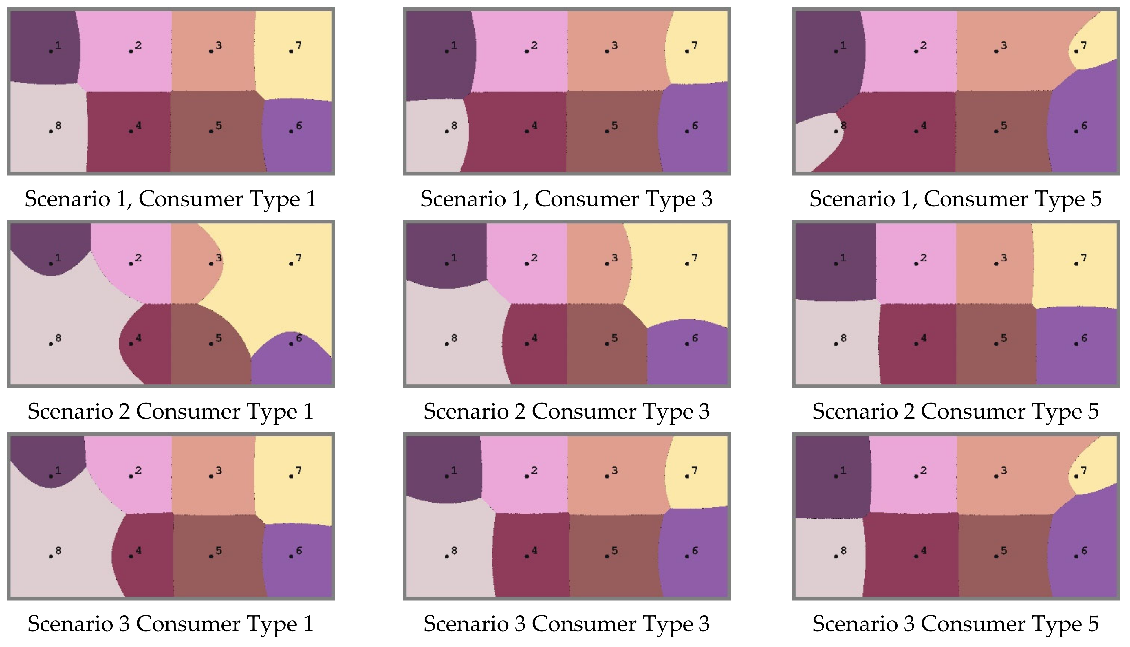
The consumer areas, obtained by solving the optimization problem, are presented in Figure 9. The four scenarios are outlined and three different consumer types based on consumers’ quality preferences are also shown. One can see how the consumer area of the firms that offer a lower-quality product decreases when the quality preferences of the consumers increase. Figure 9 also shows the estimation of demand function defined in Equation (12). In the current example, the demand function that represents the overall market share of particular firm was obtained as a weighted sum of consumer areas of this firm for each consumer type. The consumer percentages defined in Table 2 were used as weights in the sum. The equilibrium prices are shown in Table 3 and profits are shown in Table 4 and Figure 10. Profits were computed by normalizing the total output of all firms.
Firms 7 and 8 offer products of lower quality, but their equilibrium prices are higher than those of firms 2, 3, 4 and 5, in the case of a competitive market with a profit maximization strategy, i.e., Scenario 1 (Table 3). The marginal location of these firms ensures stronger market power, particularly in the presence of consumers who do not find quality important. Their location allows them to ask for higher prices than the firms in the internal area. Firms 1 and 6 have higher prices and higher profits than firms 2, 3, 4 and 5, although they offer products of the same quality and have equidistant locations also due to their marginal location. Similar behavior, but for a one-dimensional model and without vertical differentiation, was observed in [56].
Scenario 2 shows a significant decrease in the consumer area for the firms in the cartel and a significant increase in their prices. Although firms 7 and 8 are not in the cartel agreement, the Nash equilibrium provides prices that are higher than the ones obtained in Scenario 1. The firms from the cartel benefit with higher profits, but the independent firms also obtain higher profits than in Scenario 1 due to the effect known as the cartel ”umbrella”.
Scenario 3 is comparable with Scenario 1. Scenario 3 shows an increase in the consumer area of firm 8 in comparison to Scenario 1. This is expected since its strategy is market share maximization. This strategy leads to its prices being equal to its marginal cost. The prices of the firms that are located next to firm 8, i.e., firms 1 and 4, are lower, which is a consequence of the strategy of firm 8. Their profits are significantly reduced.
In Scenario 4, the cartel achieves the maximization of its profit even though firms 1 and 4 do not have any consumers from type 1. The equilibrium prices are so high that consumers from type 1 prefer to travel longer distances and to buy the product from firm 8 instead from firms 1 or 4. The comparison with Scenario 2 shows a significant decrease in the prices of the firms from the cartel and also of firm 7. As a consequence, the profits are also significantly reduced (Figure 10). This scenario outlines the strong influence that a company with a market share maximization strategy has on the profits of the cartel.
On the other hand, the comparison of Scenario 4 with Scenario 3 shows an increase in the prices of the cartel and the price of firm 7, which benefits from the cartel. Although firms 1 and 4 do not have any revenue from type 1 consumers, the cartel achieves the maximum profit from the other firms from the cartel and from firms 1 and 4, but from the rest of the consumers. These firms are located next to firm 8, which has lower prices. They lose their market share in favor of firm 8. The profits of firms 1 and 4 are reduced in comparison with Scenario 3, and these firms may prefer to leave the cartel. This type of scenario is investigated in the next sub-section.
6.2. Leaving the Cartel
It was shown in the previous sub-section that, in Scenario 4, i.e., a scenario with a cartel and a firm maximizing its market share, firms 1 and 4 from the cartel might prefer to leave it since they have a very low revenue due to their location next to the firm with the market share maximization strategy.
The Nash equilibrium is obtained by solving the optimization problem, considering that firms 1 and 4 are not in the cartel, i.e., the cartel is formed by firms 2, 3, 5 and 6, while the rest of the firms determine their prices independently: firms 1, 4 and 7 optimize their own profits and firm 8 optimizes its consumer area. The obtained equilibrium prices and profits are shown in Table 5 and Table 6, where Scenario 4 from the previous sub-section is also included for comparison. The current scenario is denoted by (p, c, c, p, c, c, p, q), where each letter corresponds to the strategy of the firm: ‘p’ denotes profit maximization, ‘c’ denotes that the firm participates in a cartel and ‘q’ denotes a market share maximization strategy. One can see that firms 1 and 4 definitely benefit from leaving the cartel and obtain higher profits. By leaving the cartel, firms 1 and 4 choose lower prices, which ensures revenue from type 1 consumers, and this increases their profits. As a result, the consumer area of the remaining firms in the cartel is reduced and consequently their profits are reduced too. The consumer areas are presented in Figure 11.
The profit of firm 2 undergoes a significant decrease. Figure 11 shows that this is due its particular location on the two-dimensional plane, where firms 1 and 4 take a significant part of its potential market share. Reducing the price by leaving the cartel might ensure a larger market share for firm 2, which in turn might lead to an increase in its profit. The Nash equilibrium was computed, considering that only firms 3–6 are in a cartel agreement while the rest of the firms determine their prices independently. The results are included in Table 5 and Table 6 and the obtained market shares are shown in Figure 11. Indeed, firm 2 increases its market share, which helps it to achieve a higher profit than when it is in the cartel. Firm 2′s decision to leave the cartel is not a direct result of the market share maximization strategy of firm 8, but rather a consequence of the decisions of firms 1 and 4, which become the main competitors of firm 2, due to its specific location on the two-dimensional plane. In one-dimensional models, one firm can interact with a maximum of two other firms and these kinds of consequences cannot be investigated.
Furthermore, the cartels of all possible combinations among firms 1 to 6 were generated and the corresponding Nash equilibriums were obtained. The results show that the cartel formed by firms 3, 5 and 6 should be the preferred one among the participants. If another firm enters or leaves the cartel, this will result in lower profits.
It is important to note that this decision to leave the cartel depends not only on the proximity of the firms’ stores to the profit maximization strategy participant, but also on the consumers’ preferences. In the case of no consumer preferences, while considering the vertical differentiation of the product, i.e., (consumers of type 5), all firms would prefer to stay in the cartel. They do not need to attract customers indifferent to the product quality by reducing their prices and they can enjoy higher profits by staying in the cartel. Thus, variability of consumer preferences and consequently their rational behavior should be appropriately handled.
A similar analysis including all possible combinations of cartels among firms 1 to 6 is generated when firm 8 follows a profit maximization strategy. In this case, all six firms would prefer to stay in the cartel, since it ensures higher profits than any other combination. Firms 1, 2, 4 and 6 might achieve higher profits if only one of them leaves the cartel, but if two or more firms leave the cartel, the profits become lower for them and thus all would prefer to remain part of the cartel.
These results clearly show that the existence of a firm with a market share maximization strategy, wherein some of the consumers are indifferent to the quality, undermines cartel stability.
6.3. Locating a New Store
This sub-section investigates the best locations for a new store. The scenario from the previous sub-section is considered, i.e., a partial cartel from firms 3–6, a profit maximization strategy for firms 1, 2, 4 and 7 and a market share maximization strategy for firm 8. It is assumed that the new store offers a lower-quality product, and two cases are analyzed. The first case considers that the new store is part of firm 7, i.e., firm 7 obtains a second store. In this case firm 7 attempts to maximize its joint profits from both stores, allowing to set different prices for each store. The second case considers that the new store is part of an independent new participant/firm on the market. The possible locations for the new store are shown in Figure 12.
The Nash equilibrium for each of these locations was computed and the locations that generate the highest profits are shown in Figure 13. Table 7 and Table 8 present equilibrium prices and profits for some of the locations shown in Figure 12 and the corresponding market shares are shown in Figure 14. The prices and profits from the stable cartel from previous section are also included in the tables for easier comparison.
One can see that firm 7 would prefer to set its new store either close to its initial location or close to firm 8. In both cases, it increases its profit by around 10%. One might assume that the locations close to the firms from the cartel would generate a higher profit. However, they generate a larger market share, but the equilibrium results show that the profit is even lower than in the case of a single store. The locations close to the first store do not challenge the cartel’s high prices and allow firm 7 to also set high prices. Contrarily, if firm 7 sets a new store closer to any of the firms from the cartel, then the Nash equilibrium results in lower prices set by the cartel, which forces firm 7 to decrease the prices of both its stores. In these cases, firm 7 achieves a larger market share, but the profits become lower than in the case of a single store. It is important to note that in all positions close to the first store of firm 7, the cartel remains stable.
The other best locations for a second store of firm 7 are located close to firm 8. They attempt to take away the market share of firm 8. Some of them are closer to firm 1. These locations benefit from the marginal location of firm 1, which offers the product at the highest price among its neighbors. Locating the new store closer to firm 1 ensures higher prices for firm 7′s product than when locating the store closer to firms 2 or 4.
Figure 13 also shows the best locations for a store for a new participant. The new participant is assumed to maximize its profit and its strategy is to compete with firm 7, which also offers a low-quality product, and to benefit from its market share. The new participant would not prefer to set its new store near firm 8 (unlike the second store of firm 7) because of the market share maximization strategy of firm 8, which results in a lower price. In this case, the new participant will be forced to reduce its price, which will provide lower profits than that of those near firm 7. Thus, the locations on the contour lines, which are at an equal distance between firms 3 and 7 and between firms 6 and 7, are not surprising. The other best locations are around firm 3. They are preferred instead of the ones around firm 6 because they ensure a larger market share. The market share around firm 3 is limited from one external border, while the market share around firm 6 is limited from two external borders. The marginal location of a new store near firm 6 does not ensure increased market power due to the close presence of another store (firm 6). Hence, the new firm cannot increase its prices without significantly decreasing its market share.
Figure 13 shows that the cartel might break up or it might remain stable for some of the best locations for firm 9. It was observed in [57] that the cartels are unstable due to the entry of a new participant to the market that leads to additional competition. The current analysis shows that new participant might enter in the market without breaking up the cartel and still obtaining one of the highest possible profits by keeping high prices due to “cartel umbrella”. The complex interactions between participants that exist in the two-dimensional space offers variability of choices for new participants. The cartel fails if the new store is located at (60, 30), while the cartel remains stable if the new store is located at (70, 20), even though these locations are equally distant from firm 7 and from the stores from the cartel. In the case of setting a new store at the first location, firm 3 prefers to leave the cartel and increase its market share to the detriment of firm 2. Meanwhile, in the second case, firm 6 cannot significantly increase its market share due to its location, and it does not obtain any benefits from leaving the cartel.
7. Conclusions
A mathematical model of an oligopoly market was developed and equilibrium prices for different scenarios were presented and analyzed. The main objective was to compare a competitive market versus a market with a cartel from one side and a maximization profit strategy versus a maximization market share strategy from another side. Horizontal and vertical product differentiation were considered by taking into account the distance between consumers and stores in a two-dimensional plane and the quality of the product. Voronoi diagrams were used to represent the market shares of each participant. It was assumed that the consumers had different quality preferences. Four different scenarios were generated, the equilibrium prices, market share and profits were obtained, and the main differences were outlined.
It was shown that stores located near the external borders of the market offer higher prices and obtain higher profits than stores located in the central part of the market area. It was also shown that the marginal location of stores near external borders with a lower-quality product is beneficial and the equilibrium prices are higher than in stores located in the central area that offer a product with higher quality.
The existence of a participant with a market share maximization strategy has a significant effect on the cartel’s profit. In a competitive market and in a market with a cartel, the existence of such a participant reduces the profits of all firms, but it has a stronger influence in reducing the profit of the cartel. The firms that are located near the participant with a market share maximization strategy yield lower profits within the cartel agreement than being independent in a competitive market, even though the collective profit of the cartel is higher. The existence of consumers with different quality preferences would force these firms to leave the cartel and increase their profits by increasing their market share of customers indifferent to quality. Otherwise, the cartel remains stable in the case of a market with consumers who insist on quality.
The best locations for the setting of a new store were shown, considering that the new store is part of an existing participant in the market or of a new participant. It was shown in both cases that the new store benefits from a partial cartel. Its location is determined in such a way that the cartel remains stable and assists in ensuring high prices at the new store. The positions of the other stores on a two-dimensional plane and the interaction between them are essential when selecting the locations that lead to the highest profits.
The analyzed examples illustrate the advantages of using a two-dimensional model. It better represents not only the real locations of stores than a one-dimensional model, but it also finds characteristics that are typical for a two-dimensional space representation that cannot be obtained by using a one-dimensional model.
Author Contributions
Conceptualization, I.K.; Methodology, I.K.; Software, S.S.; Validation, S.S.; Formal analysis, S.S; Investigation, S.S.; Writing—original draft preparation, S.S.; Writing—review and editing, I.K.; Visualization, S.S.; Supervision, I.K.; All authors have read and agreed to the published version of the manuscript.
Funding
This research received no external funding.
Data Availability Statement
No special data were used for the research apart from those described in the manuscript.
Conflicts of Interest
The authors declare no conflict of interest.
References
- Cournot, A. Researches into the Mathematical Principles of the Theory of Wealth; L. Hachette: Paris, France, 1838. [Google Scholar]
- Bertrand, J. Review of “Theorie mathematique de la richesse sociale” and “Recherche sur les principes mathematiques de la theorie des richesses”. J. Savants 1883, 67, 499–508. [Google Scholar]
- Varian, H.R. Microeconomic Analysis; W.W. Norton & Company, Inc.: New York, NY, USA, 1992. [Google Scholar]
- Hsu, J.; Wang, X.H. On Welfare under Cournot and Bertrand Competition in Differentiated Oligopolies. Rev. Ind. Organ. 2005, 27, 185–191. [Google Scholar] [CrossRef] [Green Version]
- Alipranti, M.; Milliou, C.; Petrakis, E. Price vs. quantity competition in a vertically related market. Econ. Lett. 2014, 12, 122–126. [Google Scholar] [CrossRef] [Green Version]
- Basak, D. Cournot vs. Bertrand under centralised bargaining. Econ. Lett. 2017, 54, 124–127. [Google Scholar] [CrossRef]
- Frąckiewicz, P.; Bilski, J. Quantum Games with Unawareness with Duopoly Problems in View. J. Entropy 2019, 21, 1097. [Google Scholar] [CrossRef] [Green Version]
- Tremblay, V.J.; Tremblay, C.H. New Perspectives on Industrial Organization; Springer Business and Economics: London, UK, 2012. [Google Scholar]
- Hotelling, H. Stability in competition. Econ. J. 1929, 39, 41–57. [Google Scholar] [CrossRef]
- Salop, S. Monopolistic competition with outside goods. Bell J. Econ. 1979, 10, 141–156. [Google Scholar] [CrossRef]
- Economides, N. Nash equilibrium in duopoly with products defined by two characteristics. RAND J. Econ. 1986, 17, 431–439. [Google Scholar] [CrossRef]
- Okabe, A.; Aoyagi, M. Existence of equilibrium configurations of competitive firms on an infinite two-dimensional space. J. Urban Econ. 1991, 29, 349–370. [Google Scholar] [CrossRef]
- Losch, A. The Economics of Location; Yale University Press: London, UK, 1954. [Google Scholar]
- Brown-Kruse, J.; Cronshaw, M.B.; Schenk, D. Theory and experiments on spatial competition. Econ. Inq. 1993, 31, 139–165. [Google Scholar] [CrossRef]
- Cahan, D.; Chen, H.; Christie, L.; Slinko, A. Spatial competition on 2-dimensional markets and networks when consumers don’t always go to the closest firm. Int. J. Game Theory 2021, 50, 945–970. [Google Scholar] [CrossRef]
- Eaton, B.C.; Lipsey, R.G. The non-uniqueness of equilibrium in the Loschian location model. Am. Econ. Rev. 1976, 66, 77–93. [Google Scholar]
- Capozza, D.R.; Van Order, R. A generalized model of spatial competition. Am. Econ. Rev. 1978, 68, 896–908. [Google Scholar]
- Novshek, W. Equilibrium in simple spatial (or differentiated product) models. J. Econ. Theory 1980, 22, 313–326. [Google Scholar] [CrossRef]
- Dziubiński, M. Location game on disjoint line segments. Int. J. Game Theory 2010, 40, 231–262. [Google Scholar] [CrossRef]
- Bao, L.; Yu, W. Efficiency-Enhancing Horizontal Mergers in Spatial Competition with Network Externalities. Mathematics 2022, 10, 3266. [Google Scholar] [CrossRef]
- Melitz, M.J.; Ottaviano, G. Market size, trade, and productivity. Rev. Econ. Stud. 2008, 75, 295–316. [Google Scholar] [CrossRef] [Green Version]
- Arkolakis, C.; Demidova, S.; Klenow, P.J.; Rodriguez-Clare, A. Endogenous variety and the gains from trade. Am. Econ. Rev. 2008, 98, 444–450. [Google Scholar] [CrossRef] [Green Version]
- Li, C.; Ji, X. Innovation, licensing, and price vs. quantity competition. Econ. Model. 2010, 27, 746–754. [Google Scholar] [CrossRef]
- Lahmandi-Ayed, R. Spatial differentiation, divisible consumption and the pro-competitive effect of income. J. Math. Econ. 2010, 46, 71–85. [Google Scholar] [CrossRef]
- Askar, S.S.; Al-khedhairi, A. Dynamic investigations in a duopoly game with price competition based on relative profit and profit maximization. J. Comput. Appl. Math. 2020, 367, 112464. [Google Scholar] [CrossRef]
- Kishihara, H.; Matsubayashi, N. Product Repositioning in a Horizontally Differentiated Market, Rev. Ind. Org. 2020, 57, 701–718. [Google Scholar] [CrossRef]
- Liu, L.; Wang, X.H.; Zeng, C. Endogenous horizontal product differentiation in a mixed duopoly. Rev. Ind. Organ. 2020, 56, 435–462. [Google Scholar] [CrossRef]
- Brady, M. Asymmetric Horizontal Differentiation under Advertising in a Cournot Duopoly. Games 2022, 13, 37. [Google Scholar] [CrossRef]
- Garrod, L.; Olczak, M. Explicit vs. tacit collusion: The effects of firm numbers and asymmetries. Int. J. Ind. Organ. 2018, 56, 1–25. [Google Scholar] [CrossRef] [Green Version]
- Fonseca, M.; Normann, H.T. Explicit vs. tacit collusion—The impact of communication in oligopoly experiments. Eur. Econ. Rev. 2012, 56, 1759–1772. [Google Scholar] [CrossRef] [Green Version]
- Kuipers, J.; Olaizola, N. A dynamic approach to cartel formation, Int. J. Game Theory 2008, 37, 397–408. [Google Scholar] [CrossRef] [Green Version]
- Gabszewicz, J.J.; Marini, M.A.; Tarola, O. Vertical differentiation and collusion: Pruning or proliferation? Res. Econ. 2017, 71, 129–139. [Google Scholar] [CrossRef] [Green Version]
- Correani, L.; Dio, F. A note on link formation and network stability in a Hotelling game. Oper. Res. Lett. 2017, 45, 289–292. [Google Scholar] [CrossRef]
- Bos, I.; Marini, M. Cartel stability under quality differentiation. Econ. Lett. 2019, 174, 70–73. [Google Scholar] [CrossRef] [Green Version]
- Song, R.; Wang, L. Collusion in a differentiated duopoly with network externalities. Econ. Lett. 2017, 152, 23–26. [Google Scholar] [CrossRef]
- Biancini, S.; Ettinger, D. Vertical integration and downstream collusion. Int. J. Ind. Organ. 2017, 53, 99–113. [Google Scholar] [CrossRef] [Green Version]
- Grisáková, N.; Štetka, P. Cournot’s Oligopoly Equilibrium under Different Expectations and Differentiated Production. Games 2022, 13, 82. [Google Scholar] [CrossRef]
- Buzzell, R.D.; Gale, B.T.; Sultan, R.G.M. Market share: A key to profitability. Harvard Bus. Rev. 1975, 53, 97–106. [Google Scholar]
- Askar, S.S. A Dynamic Duopoly Model: When a Firm Shares the Market with Certain Profit. Mathematics 2020, 8, 1826. [Google Scholar] [CrossRef]
- Porter, M.E. Competitive Strategy—Techniques for Analyzing Industries and Competitors; The Free Press: New York, NY, USA, 1980. [Google Scholar]
- Ward, P.T.; Bickford, D.J.; Leong, G.K. Configurations of manufacturing strategy, business strategy, environment and structure. J. Manag. 1996, 22, 597–626. [Google Scholar] [CrossRef]
- Venkatraman, N. Strategic orientation of business enterprises: The construct, dimensionality and measurement. Managem. Sci. 1989, 35, 942–962. [Google Scholar] [CrossRef] [Green Version]
- Mintzberg, H. Generic strategy: Toward a comprehensive framework. Adv. Strategic Manag. 1988, 5, 1–67. [Google Scholar]
- Jiang, J.; Shi, Y.; Wang, X.; Chen, X. Regularized two-stage stochastic variational inequalities for Cournot-Nash equilibrium under uncertainty. J. Comp. Math. 2019, 37, 813–842. [Google Scholar] [CrossRef]
- Outrata, J.V.; Ferris, M.C.; Červinka, M.; Outrata, M. On Cournot-Nash-Walras equilibria and their computation. Set-Valued Var. Anal. 2016, 24, 387–402. [Google Scholar] [CrossRef]
- Ledvina, A.; Sircar, R. Dynamic Bertrand Oligopoly. Appl. Math. Optim. 2011, 63, 11–44. [Google Scholar] [CrossRef] [Green Version]
- Zhu, Y.; Zhou, W.; Chu, T.; Elsadany, A. Complex dynamical behavior and numerical simulation of a Cournot-Bertrand duopoly game with heterogeneous players. Commun. Nonlinear Sci. Numer. Simulat. 2021, 101, 105898. [Google Scholar] [CrossRef]
- Ma, J.; Si, F. Complex dynamics of a continuous Bertrand duopoly game model with two-stage delay. Entropy 2016, 18, 266. [Google Scholar] [CrossRef] [Green Version]
- Ahmed, E.; Elsadanym, A.; Puu, T. On Bertrand duopoly game with differentiated goods. Appl. Math. Comp. 2015, 251, 169–179. [Google Scholar] [CrossRef]
- Corriou, J.-P. Numerical Methods and Optimization: Theory and Practice for Engineers; Springer: Berlin/Heidelberg, Germany, 2021. [Google Scholar]
- Barzilai, J.; Borwein, J. Two-Point Step Size Gradient Methods. IMA J. Numer. Anal. 1988, 8, 141–148. [Google Scholar] [CrossRef]
- Aurenhammer, F.; Klein, R.; Lee, D.-T. Voronoi Diagrams and Delaunay Triangulations; World Scientific Publishing Co.: Singapore, 2013. [Google Scholar]
- Geuzaine, C.; Remacle, J.F. Gmsh: A three-dimensional finite element mesh generator with built-in pre- and post-processing facilities. Int. J. Numer. Meth. Eng. 2009, 79, 1309–1331. [Google Scholar] [CrossRef]
- Boris, S.M. Multiobjective optimization problems with equilibrium constraints. Math. Program. Ser. B. 2009, 117, 331–354. [Google Scholar] [CrossRef] [Green Version]
- Bos, I.; Marini, M.; Saulle, R. Cartel formation with quality differentiation. Math. Social Sci. 2020, 106, 36–50. [Google Scholar] [CrossRef] [Green Version]
- Brenner, S. Hotelling games with three, four, and more players. J. Reg. Sci. 2005, 45, 851–864. [Google Scholar] [CrossRef] [Green Version]
- Grossman, P.Z. How Cartels Endure and How They Fail: Studies of Industrial Collusion; Edward Elgar Publishing: Cheltenham, UK, 2004. [Google Scholar]
Figure 1.
Sample mesh of a rectangular area.

Figure 2.
Convergence with mesh size. (a) Absolute error of price vector; (b) prices of two firms.

Figure 3.
Convergence of the iterative optimization method. (a) Mesh 1; (b) Mesh 4.

Figure 4.
Convergence of the iterative optimization method with adaptive step and vertical differentiation products, Mesh 4.
Figure 4.
Convergence of the iterative optimization method with adaptive step and vertical differentiation products, Mesh 4.

Figure 5.
Smoothness of consumer areas with mesh refinement. Dots denote locations of stores of 8 different firms.
Figure 5.
Smoothness of consumer areas with mesh refinement. Dots denote locations of stores of 8 different firms.

Figure 6.
Profit of the cartel as function of quality of the product.

Figure 7.
Sensitivity analysis of parameters (a) , (b) and (c) defined in the utility function.

Figure 8.
Map showing the locations of each store of the 8 firms.

Figure 9.
Comparison of consumer areas of all scenarios.


Figure 10.
Profits in each scenario. The profits are obtained based on the normalized total output of all firms. Profits of firms 1 to 6 are accumulated.
Figure 10.
Profits in each scenario. The profits are obtained based on the normalized total output of all firms. Profits of firms 1 to 6 are accumulated.

Figure 11.
Comparison of consumer areas of Scenario 4 with different cartel structures.


Figure 12.
Locations of stores of the incumbent eight firms and (★) possible locations for a new store.
Figure 12.
Locations of stores of the incumbent eight firms and (★) possible locations for a new store.

Figure 13.
(★) Best locations for a new store of firm 7; (★) best locations for a new store of the ninth participant; (☆) best locations for a new store of the ninth participant where the cartel would fail.
Figure 13.
(★) Best locations for a new store of firm 7; (★) best locations for a new store of the ninth participant; (☆) best locations for a new store of the ninth participant where the cartel would fail.

Figure 14.
Consumer areas of when new store is added, consumers type 3.


Table 1.
Properties of meshes used for convergence study; represents average element edge.
| Nodes | Triangles | ||
|---|---|---|---|
| Mesh 1 | 1092 | 2122 | 0.54 |
| Mesh 2 | 4364 | 8488 | 1.07 |
| Mesh 3 | 17,213 | 33,952 | 2.14 |
| Mesh 4 | 68,369 | 135,808 | 4.29 |
| Mesh 5 | 272,513 | 543,232 | 8.57 |
Table 2.
Different types of consumer quality preferences.
| Consumer Type | Percentage of the Consumers | |
|---|---|---|
| Type 1 | 0 | 10% |
| Type 2 | 0.25 | 20% |
| Type 3 | 0.5 | 40% |
| Type 4 | 0.75 | 20% |
| Type 5 | 1 | 10% |
Table 3.
Prices of the Nash equilibrium.
| Firm | Scenario 1 | Scenario 2 | Scenario 3 | Scenario 4 |
|---|---|---|---|---|
| Firm 1 | 2.147 | 2.509 | 2.092 | 2.240 |
| Firm 2 | 2.046 | 2.509 | 2.048 | 2.240 |
| Firm 3 | 2.050 | 2.509 | 2.052 | 2.240 |
| Firm 4 | 2.050 | 2.509 | 2.022 | 2.240 |
| Firm 5 | 2.046 | 2.509 | 2.041 | 2.240 |
| Firm 6 | 2.147 | 2.509 | 2.144 | 2.240 |
| Firm 7 | 2.080 | 2.211 | 2.081 | 2.150 |
| Firm 8 | 2.080 | 2.211 | 1.84 | 1.84 |
Table 4.
Profits of the Nash equilibrium.
| Firm | Scenario 1 | Scenario 2 | Scenario 3 | Scenario 4 |
|---|---|---|---|---|
| Firm 1 | 0.027 | 0.056 | 0.015 | 0.014 |
| Firm 2 | 0.023 | 0.072 | 0.019 | 0.031 |
| Firm 3 | 0.026 | 0.056 | 0.026 | 0.045 |
| Firm 4 | 0.026 | 0.056 | 0.015 | 0.014 |
| Firm 5 | 0.023 | 0.072 | 0.022 | 0.041 |
| Firm 6 | 0.027 | 0.056 | 0.027 | 0.045 |
| Firm 7 | 0.017 | 0.069 | 0.017 | 0.032 |
| Firm 8 | 0.017 | 0.069 | 0.003 | 0.006 |
Table 5.
Prices of the Nash equilibrium.
| Firm | (c, c, c, c, c, c, p, q) | (p, c, c, p, c, c, p, q) | (p, p, c, p, c, c, p, q) |
|---|---|---|---|
| Firm 1 | 2.240 | 2.097 | 2.092 |
| Firm 2 | 2.240 | 2.252 | 2.055 |
| Firm 3 | 2.240 | 2.252 | 2.235 |
| Firm 4 | 2.240 | 2.051 | 2.033 |
| Firm 5 | 2.240 | 2.252 | 2.235 |
| Firm 6 | 2.240 | 2.252 | 2.235 |
| Firm 7 | 2.150 | 2.155 | 2.148 |
| Firm 8 | 1.84 | 1.84 | 1.84 |
Table 6.
Profits of the Nash equilibrium.
| Firm | (c, c, c, c, c, c, p, q) | (p, c, c, p, c, c, p, q) | (p, p, c, p, c, c, p, q) |
|---|---|---|---|
| Firm 1 | 0.014 | 0.022 | 0.016 |
| Firm 2 | 0.031 | 0.018 | 0.027 |
| Firm 3 | 0.045 | 0.042 | 0.031 |
| Firm 4 | 0.014 | 0.033 | 0.024 |
| Firm 5 | 0.041 | 0.027 | 0.025 |
| Firm 6 | 0.045 | 0.046 | 0.045 |
| Firm 7 | 0.032 | 0.033 | 0.031 |
| Firm 8 | 0.006 | 0.004 | 0.003 |
Table 7.
Equilibrium prices after locating a new store.
| Firm | Stable Cartel | Firm 7 with New Store | Firm 9 | ||
|---|---|---|---|---|---|
| (65, 35) | (20, 20) | (60, 30) | (70, 20) | ||
| Firm 1 | 2.092 | 2.092 | 2.088 | 2.092 | 2.092 |
| Firm 2 | 2.055 | 2.056 | 2.029 | 2.055 | 2.054 |
| Firm 3 | 2.235 | 2.232 | 2.227 | 2.120 | 2.112 |
| Firm 4 | 2.033 | 2.033 | 2.024 | 2.033 | 2.032 |
| Firm 5 | 2.235 | 2.232 | 2.227 | 2.120 | 2.112 |
| Firm 6 | 2.235 | 2.232 | 2.227 | 2.120 | 2.112 |
| Firm 7 | 2.148 | 2.168 | 2.144 | 2.013 | 2.013 |
| Firm 8 | 1.84 | 1.84 | 1.84 | 1.84 | 1.84 |
| Firm 7/9 | - | 2.155 | 1.913 | 1.946 | 1.943 |
Table 8.
Profits after locating a new store.
| Firm | Stable Cartel | Firm 7 with New Store | Firm 9 | ||
|---|---|---|---|---|---|
| (65, 35) | (20, 20) | (60, 30) | (70, 20) | ||
| Firm 1 | 0.016 | 0.016 | 0.013 | 0.016 | 0.016 |
| Firm 2 | 0.027 | 0.027 | 0.022 | 0.022 | 0.021 |
| Firm 3 | 0.031 | 0.027 | 0.028 | 0.011 | 0.023 |
| Firm 4 | 0.024 | 0.024 | 0.020 | 0.018 | 0.018 |
| Firm 5 | 0.025 | 0.025 | 0.024 | 0.020 | 0.020 |
| Firm 6 | 0.045 | 0.046 | 0.044 | 0.027 | 0.014 |
| Firm 7 | 0.031 | 0.035 | 0.035 | 0.009 | 0.009 |
| Firm 8 | 0.003 | 0.003 | 0.003 | 0.003 | 0.003 |
| Firm 9 | - | - | - | 0.008 | 0.008 |
Disclaimer/Publisher’s Note: The statements, opinions and data contained in all publications are solely those of the individual author(s) and contributor(s) and not of MDPI and/or the editor(s). MDPI and/or the editor(s) disclaim responsibility for any injury to people or property resulting from any ideas, methods, instructions or products referred to in the content. |
© 2023 by the authors. Licensee MDPI, Basel, Switzerland. This article is an open access article distributed under the terms and conditions of the Creative Commons Attribution (CC BY) license (https://creativecommons.org/licenses/by/4.0/).
Share and Cite
MDPI and ACS Style
Stoykov, S.; Kostov, I. Price Competition with Differentiated Products on a Two-Dimensional Plane: The Impact of Partial Cartel on Firms’ Profits and Behavior. Games 2023, 14, 24. https://doi.org/10.3390/g14020024
AMA Style
Stoykov S, Kostov I. Price Competition with Differentiated Products on a Two-Dimensional Plane: The Impact of Partial Cartel on Firms’ Profits and Behavior. Games. 2023; 14(2):24. https://doi.org/10.3390/g14020024
Chicago/Turabian StyleStoykov, Stanislav, and Ivan Kostov. 2023. "Price Competition with Differentiated Products on a Two-Dimensional Plane: The Impact of Partial Cartel on Firms’ Profits and Behavior" Games 14, no. 2: 24. https://doi.org/10.3390/g14020024
Note that from the first issue of 2016, this journal uses article numbers instead of page numbers. See further details here.