Computer Solution to the Game of Pure Strategy

Abstract

We numerically solve the classical “Game of Pure Strategy” using linear programming. We notice an intricate even-odd behaviour in the results of our computations that seems to encourage odd or maximal bids.

1. Introduction

Simple, two-player games are important models for human decision making. They should have sufficiently elementary rules so that they can be studied both theoretically and empirically, yet be sufficiently rich to involve a non-trivial amount of human psychological experience.

We study, and solve numerically, the “Game of Pure Strategy”. The solution is not implementable by a human, but only by a computer. The game is a model of decision making based on bidding, which is an important paradigm in game theory, because it can easily be shown (see below) that no deterministic strategy may succeed.

We notice, in the numerical data, that the optimal probabilities of the bids do not follow a unimodal pattern; indeed the parity of the bid is often more important than its actual value. This echoes a known recommendation for online bidding (in which the bidding amounts are less restricted than in room bidding): the website http://www.bidnapper.com recommends to its customers to “Bid in odd amounts. Many novices bid in rounded numbers.”.

2. The Game of Pure Strategy

Goofspiel, also called Game of Pure Strategy (GOPS) is a two person game. Take a standard 52 card deck and discard all of the cards of one suit. The cards of one suit are given to one player, the cards of another suit are given to the other player, and the cards in the remaining suit are shuffled and placed face down in the middle. The cards are valued from low to high as ace = 1, 2, 3, ..., 10, jack = 11, queen = 12, and king = 13.

A round consists of turning up the next card from the middle pile and then the two players “bet” on the upturned card, each player choosing one card and then simultaneously displaying it to the other player. The player showing the highest card wins the value of the upturned card. If both players display the same card, the point value is split between the two players. These three cards are then discarded. The game ends after 13 rounds and the winner is the person who obtained the most points (one needs 46 points or more to win).

Though the mechanics of the game are simple, the strategy is not. Suppose for example that the king is the upturned card in the first round. Further suppose that you choose to bet one (i.e., the ace). When you turn your card up, you found out that your opponent bet his king winning 13 points. You are happy with this result because you now have 12 more betting points, which should more than make up for the lost 13 points. In fact, it is possible that you could win every remaining point by always betting one more than your opponent (though of course that would require cheating, by knowing in advance what your opponent is going to bet). However, you are taking a chance by betting only one: if your opponent had bet a two or three, then he would have won 13 points at almost no cost. When playing the game you are trying to outguess your opponent while your opponent is trying to outguess you: you find yourself reasoning along lines such as “my opponent is probably going to play X so I should play Y, but he may see through this and instead play Z to defeat Y so maybe I should play W instead.”

3. Solving GOPS

To be able to solve GOPS using game theory, we use an equivalent scoring system: the player with the higher card wins from the opponent the value of the upturned card, or wins nothing in the event of a tie. The game is now a two-person zero-sum game that can be represented by a matrix with one row for each possible play of player one and one column for each possible play of player two. The i, j’th entry of the matrix is the value of the game to player one when player one makes his i’th play while player two makes his j’th play (such a formulation is called a matrix game).

It is not hard to see that one should not choose a deterministic strategy. In fact, every deterministic strategy A can be defeated as follows. Use strategy A to find the card that my opponent is going to play. If my opponent is going to play a king, play the ace. Otherwise play the card that is one higher than my opponent’s choice. This counterstrategy will win every round except one resulting in a trouncing. Instead the strategy should have some random variations where one plays particular cards with some probability.

How difficult is it to analyze this game? Suppose the cards are valued from 1 through N. The number of distinct ways that the middle suit could be ordered and the number of distinct betting sequences for each player are N factorial. Hence, the number of possible ways of playing out a game is f (N) = (N!)³. Analysis of GOPS, along these lines, would require consideration, for N = 13, of 2.4 × 10²⁹ variations, a number clearly beyond computational possibilities.

To our knowledge, the game had never been previously analyzed beyond N = 5, see [1]. There is a way to significantly reduce the number of games needed to be analyzed. Sheldon Ross [2] describes a recursive rule expressing the value of a game as a function of the values of smaller games. We give a further simplification of his rule.

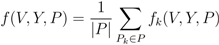
Let f (V, Y, P) be the value for player one of the game in which V is the set of cards player one has in his hand, Y is the set of cards player two has in his hand, and P is the set of cards in the deck. Further, for P_k ∈ P, let f_k(V, Y, P) be the value for player one of that game, once the upcard P_k has been revealed. Clearly f (V, Y, P) is the average of the f_k(V, Y, P):

Suppose |V|=|Y|=|P|= N. Then f_k(V, Y, P) is expressed as the value of the N × N game whose payoff matrix [X_ij] is

here

In English, this self-evident rule says the value of the game when player one plays V_i and player two plays Y_j is the value of the upturned card that is won or lost, plus the average value of the remaining game where the average is taken over all possible remaining upturned cards.

Blindly applying this rule results in a straightforward recursive program; however, evaluation of f (V, Y, P) on sets of cardinality N requires N³ evaluations of f on sets of cardinality N − 1, leading again to the (N!)³ complexity estimate.

To avoid this issue, we use a bottom-up approach storing the values f (V, Y, P) of the subgames as we go. We use these stored values when computing the larger subgames. Using this standard technique, called dynamic programming, we compute the value of each subgame only once. For an initial N × N game, this reduces the number of subgames that we need to solve and store to , a much more feasible number. Furthermore, we may use the symmetry between players one and two to gain an extra factor of two, since f (V, Y, P) = − f (V, Y, P) and f (V, Y, P) = 0; and at each step of the algorithm we only need to store in memory the values of f (V, Y, P) for a given value of j. On a large computer with 1 TB core memory, the game is then solvable up to N = 16.

3.1. Linear Programs

Linear programming is a standard technique. For the sake of completeness, we are going to explain how to use linear programming to solve a matrix game such as GOPS. Readers already familiar with this technique may wish to skip this section.

If all values f (V, Y, P) are known, it is then easy to compute the optimal playing strategy. Let us say that the remaining cards are V, Y, P respectively for player one, player two and the deck, and that P_k ∈ P has been turned up. Recall the payoff matrix [X_ij] from the previous subsection. The optimal strategy, for player one, will take the form of a list of probabilities x_i of playing card V_i. Assuming that player two plays optimally, we want to maximize ; namely, we want to maximize the outcome, allowing player two to make the best move (i.e., minimize the outcome) as long as he does not know our move. The solution is then a Nash equilibrium of the game.

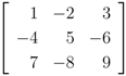
This maximization problem is a linear program (LP), and we will solve it using linear programming tools. The classical reference [3] remains an excellent introduction to linear programming. For example, suppose we have the following 3 × 3 matrix game:

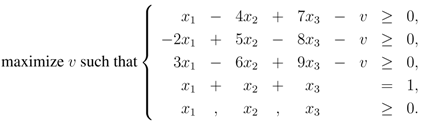
To formulate this as a LP, we introduce the variables x₁, x₂, and x₃ to represent the probabilities with which player one should play columns 1, 2 and 3 respectively. We also introduce the variable v to represent the value of the game. The LP formulation of this game is as follows:

The last two constraint rows are needed to ensure that x₁, x₂ and x₃ form a probability distribution. The variable v is unrestricted. Note that we are maximizing the expected profit, not the probability of winning. If we are playing for money, and there is some agreed-upon amount per point won, then this is the optimal strategy. If, however, we want to maximize the probability of winning, and not the amount won, then the results may be different.

Indeed, suppose the remaining cards are queen, king, player one has 2,4 in his hand, and player two has ace, 3 in her hand. Player one can guarantee victory by always playing 4 when the king shows up, but by doing so forfeits the chance of winning both last cards and guarantees a win by only one point. Playing either card with the same probability gives him an average gain of 12.5 (the optimal strategy is to play high with 52% probability on the king, resulting in an average gain of 12.52).

There is a single 0 × 0 game, whose value is 0, and it may be used to start the induction with f (Ø,Ø,Ø) = 0. We note that, up to games, 2 × 2 the results are easily computed by hand. Trivially, a 1 × 1 game is won by the player having the largest card. Consider the following 2 × 2 matrix game:

If a value is a minimum value in its column and a maximum value in its row, then it is a saddle point. If the game has a saddle point, then the value of the game is the value of a saddle point entry (there may be more than one saddle point). If the game has no saddle point, then the value of the game is (ad − bc)/(a - b - c + d). The formulation of a matrix game as a LP and the solution to 2 × 2 matrix games can be found in many sources (e.g., [4]).

4. Results

We have computed the winning strategies for N = 13 using the method described in the previous section: for each triple V, Y, P of subsets of {1,...,13} of same cardinality, we have computed the value f (V, Y, P) of the corresponding game, and have computed the probability arrays x_ki with which card V_i should be played if the upcard is P_k.

Because of its formulation as a maximization of a piecewise-linear function, these probabilities are rational numbers. We shall argue that their denominators are so large as to make exact computations pointless.

4.1. Implementation

We use the publicly available GLPK linear programming solver to solve repeatedly the matrix games. This package implements the simplex algorithm both in floating-point and multi-precision rational arithmetic.

In our computer program, we represent the card sets by bit-vectors. To conserve space, we use a perfect hash table, i.e., a table whose entries correspond bijectively to subgames. The subgames are stored in lexicographic order; each subgame is represented by the concatenation of the representations of player 1’s hand, player 2’s hand, and the deck. When we need the value of a previously computed subgame, we compute its position in our ordering and grab the corresponding entry from the table. In our dynamic programming method, we compute subgames in increasing size of hands. To conserve space, we only store the results of the subgames of the current size that we are working on and the subgames of the next smaller size. This is possible because the value of a subgame is needed only when computing the values of subgames of the next larger size.

The results do not get interesting until N = 5. There, in the initial position, the optimal betting strategies, rounded to four digits, are

Table 1. Optimal strategy at the first move, N = 5.

	upcard
	1	2	3	4	5
1	0.0470	0.1855	0.1182	0.1226	0.1123
2	0.8327	0	0.1188	0.07347	0.0241
3	0.1203	0.7375	0	0.1915	0
4	0	0.0770	0.7630	0.2043	0
5	0	0	0	0.4081	0.8636

Table 1. Optimal strategy at the first move, N = 5.

	upcard
	1	2	3	4	5
1	0.0470	0.1855	0.1182	0.1226	0.1123
2	0.8327	0	0.1188	0.07347	0.0241
3	0.1203	0.7375	0	0.1915	0
4	0	0.0770	0.7630	0.2043	0
5	0	0	0	0.4081	0.8636

The exact values, as pointed before, are prohibitively long to write down. For example, the top entry 0.0470 is really

We have computed the exact values up to N = 7; the numerators and denominators of the optimal probabilities have approximately one million digits.

Table 2. Optimal strategy at the first move, N = 13.

	upcard
	1	2	3	4	5	6	7	8	9	10	11	12	13
1	0	0	.052	.031	0	0	.020	0	0	0	.014	0	.010
2	.414	.227	0	.020	.056	.073	0	.034	.047	.036	0	.030	0
3	.090	.022	.178	.095	.036	.002	.069	.021	.002	0	.041	0	.037
4	.496	.299	.034	.061	.088	.098	0	.054	.065	.067	0	.056	0
5	0	.098	.230	.134	.067	0	.124	.039	0	0	.080	0	.065
6	0	.355	.092	.107	.124	.185	0	.077	.120	.098	0	.082	0
7	0	0	.274	.175	.101	.002	.168	.060	.001	0	.102	.008	.087
8	0	0	.139	.154	.165	.218	.021	.103	.142	.138	.016	.099	0
9	0	0	0	.221	.148	.045	.202	.092	.029	.015	.123	.028	.126
10	0	0	0	0	.215	.266	0	.144	.177	.170	0	.124	.013
11	0	0	0	0	0	.110	.397	.151	0	.063	.253	.065	0
12	0	0	0	0	0	0	0	.226	.417	.241	.023	0	0
13	0	0	0	0	0	0	0	0	0	.170	.348	.508	.661

Table 2. Optimal strategy at the first move, N = 13.

	upcard
	1	2	3	4	5	6	7	8	9	10	11	12	13
1	0	0	.052	.031	0	0	.020	0	0	0	.014	0	.010
2	.414	.227	0	.020	.056	.073	0	.034	.047	.036	0	.030	0
3	.090	.022	.178	.095	.036	.002	.069	.021	.002	0	.041	0	.037
4	.496	.299	.034	.061	.088	.098	0	.054	.065	.067	0	.056	0
5	0	.098	.230	.134	.067	0	.124	.039	0	0	.080	0	.065
6	0	.355	.092	.107	.124	.185	0	.077	.120	.098	0	.082	0
7	0	0	.274	.175	.101	.002	.168	.060	.001	0	.102	.008	.087
8	0	0	.139	.154	.165	.218	.021	.103	.142	.138	.016	.099	0
9	0	0	0	.221	.148	.045	.202	.092	.029	.015	.123	.028	.126
10	0	0	0	0	.215	.266	0	.144	.177	.170	0	.124	.013
11	0	0	0	0	0	.110	.397	.151	0	.063	.253	.065	0
12	0	0	0	0	0	0	0	.226	.417	.241	.023	0	0
13	0	0	0	0	0	0	0	0	0	.170	.348	.508	.661

Although only the first move of the optimal strategy is given, it already points to some interesting and surprising properties. The probabilities are not at all unimodal; on the contrary, they exhibit an even-odd phenomenon. If the upcard N is large (> 9), then one should not bet a card < N/2 and of opposite parity. It is striking that, in the last column, odd bets are consistently (up to i = 10) preferred over even bets; and that, in general, one should bet a card of the same parity as the upcard.

For small upcards, one should sometimes bet a counterintuitively high amount. If the upcard is a 1, one should never bet a 1 but should bet a 4 nearly 50% of the time! When the upcard is a 2, one should never bet a 1 but should bet a 6 about 35% of the time! When the upcard is a 3, one should sometimes bet as much as an 8! Mysteriously, one’s initial bet should be a 1 only when the upcard is a 3, 4, 7, 11 or 13.

The tables we do not show (available at http://gcrhoads.byethost4.com/gops.html) are similarly mysterious and surprising, and have only a couple of common properties. For the N-card game (N = 5,...,13), when the initial card is an N, one should never bet N − 1 nor N − 2. Also when the initial card is N and N is even, one should never bet a 1. Other than that each table bears little resemblance to the others.

5. Outlook

The first author made a version of the program that stored the actual probability vectors associated with the optimal strategies. These strategies were then used in a simple program that actually played the 9-card game. Despite the counterintuitive nature of these results, the computer player did win the majority of the games.

If one attempts to maximize the probability of winning instead of amount won, then there is at least one weakness in the computed strategies. In the 9-card game, suppose the initial upcard is a 9. The computer player will play a 9 with a probability, rounded to four digits, of 0.7475. Now if the human always plays 1, then nearly 3/4 of the time he will gain an advantage: playing 1 against the computer’s 9 is to his advantage due to his increased betting strength for the remainder of the game. The computed strategies optimize the amount won, and not the probability of winning. When one plays 1 against the computed strategies, then in a minority of cases the computer will play a small value, keeping its 9 and gaining more of an advantage than one stands to get when the computer chooses to play 9. The optimal strategies for maximizing the probability of winning are still unknown.

Our computer code was run on a 64-bit computer with 160 nodes and 640 GB core memory. It relies on the GLPK linear programming library. It is available at http://www.uni-math.gwdg.de/laurent/gops.zip as a C++ program.