Game Theoretic Interaction and Decision: A Quantum Analysis

1
Mathematisches Institut, Universität zu Köln, Weyertal 80, 50931 Köln, Germany
2
Paris School of Economics, University of Paris I, 106-112, Bd. de l’Hôpital, 75013 Paris, France
*
Author to whom correspondence should be addressed.
Games 2017, 8(4), 48; https://doi.org/10.3390/g8040048
Submission received: 12 July 2017
/
Revised: 19 October 2017
/
Accepted: 21 October 2017
/
Published: 6 November 2017
Abstract
:An interaction system has a finite set of agents that interact pairwise, depending on the current state of the system. Symmetric decomposition of the matrix of interaction coefficients yields the representation of states by self-adjoint matrices and hence a spectral representation. As a result, cooperation systems, decision systems and quantum systems all become visible as manifestations of special interaction systems. The treatment of the theory is purely mathematical and does not require any special knowledge of physics. It is shown how standard notions in cooperative game theory arise naturally in this context. In particular, states of general interaction systems are seen to arise as linear superpositions of pure quantum states and Fourier transformation to become meaningful. Moreover, quantum games fall into this framework. Finally, a theory of Markov evolution of interaction states is presented that generalizes classical homogeneous Markov chains to the present context.
1. Introduction
In an interaction system, economic (or general physical) agents interact pairwise, but do not necessarily cooperate towards a common goal. However, this model arises as a natural generalization of the model of cooperative TU games, for which already Owen [1] introduced the co-value as an assessment of the pairwise interaction of two cooperating players1. In fact, it turns out that the context of interaction systems provides an appropriate framework for the analysis of cooperative games (cf. Faigle and Grabisch [3]). It is therefore of interest to investigate interaction systems in their own right.
A second motivation comes from strong arguments (put forth most prominently by Penrose [4]) that the human mind with its decisions and actions constitutes a physical quantum system and should therefore be modelled according to the laws of quantum mechanics. This idea has furthered a seemingly new and rapidly growing branch of game theory where in so-called quantum games the players are assumed to execute actions on quantum systems according to the pertinent laws of physics2. The actions of the quantum players typically transform quantum bit vectors according to the same mechanisms attributed to so-called quantum computers. Many classical games of economic or behavioral interest have been studied in this setting. The Prisoners’ Dilemma, for example, has been found to offer a Pareto optimal Nash equilibrium in the quantum model where no such equilibrium exists in the classical variant (Eisert et al. [7]).
The quantum games discussed in the literature are generally non-cooperative. Although cooperative game theory has been applied to quantum theory3, a cooperative quantum game theory has not really developped4. In general, it is felt that quantum game theory has a highly physical side to it5 and that there is a gap between physics and rational game theoretic behavior6.
Therefore, it may be surprising that the mathematical analysis of interaction systems exhibits no conceptual gap to exist between the “classical” and the “quantum” world in game theory. In particular, no special knowledge of quantum mechanics (or physics in general) is needed to understand game theoretic behavior mathematically. Both aspects are faces of the same coin. The quantum aspects arise from the choice of terminology in the mathematical structural analysis rather than from innately physical environments. However, much structural insight is gained from the study of classical interaction and decision systems in terms of quantum theoretical language.
The key in the analysis is the symmetry decomposition of the matrix of interaction coefficients associated with a state of an interaction system. The decomposition allows us to represent states by self-adjoint matrices. Spectral decomposition then shows that interaction states have real eigenvalues. Moreover, each state is represented by a linear combination of pure density matrices. The connection to physical quantum models is now immediate: the axioms of quantum theory stipulate that quantum states can be described as convex combinations of pure density matrices. It follows that interaction systems subsume (finite-dimensional) quantum systems as special cases. We develop the mathematical details in Section 2 and Section 3. Section 4 treats measurements on interaction systems as linear functionals on the space of interaction matrices and provides a probabilistic interpretation that is commensurate with the probabilistic interpretation of measurements in standard physical quantum theory.
Section 5 approaches a binary decision system with a single decision maker as a system with two ”interacting” alternatives. Decision systems with n decision makers arise as tensor products of n single decision systems. Again, the relation with quantum models is immediate: The states of an n-decision system are described by complex n-dimensional vectors of unit length in exactly the same way as such vectors are assumed to describe the states of an n-dimensional quantum system in the Schrödinger picture of quantum theory.
The latter yields a very intuitive interpretation of quantum games: the players select their strategies as to move some decision makers into accepting an alternative that offers financial rewards to the individual players, where the financial reward is given as a linear functional on the space to decision states (Section 5.4).
The choice of a set-theoretic representation of the decision states shows how classical cooperative TU games may be viewed as particular decision states of a finite set of decision makers. The associated probabilistic interpretation exhibits in particular Aubin’s [13] fuzzy games as decision instances where the decision makers (or “players”) take their decisions probabilistically but independently from one another.
The model of quantum computing7 views computation as the application of certain linear operators on quantum states. We point out in Section 5.3 how well-known linear transformations (e.g., Möbius or Walsh transform) in cooperative games theory arise as tensor products of simple transformations on single decision systems. Moreover, we show that the classical Fourier transform is well-defined in the context of interaction systems, while it does not seem to exist when attention is restricted to the classical space of TU games.
We finally present a linear model for the evolution of interaction systems and discuss its “Markovian” aspects. In addition to the application examples in the course of the treatment, the appendix contains a worked out example of an interaction system with two agents. The discussion is restricted to finite-dimensional systems. An extension to infinite systems is outlined in Section 7.
The main points of our contribution are:
- Interaction systems provide a general model for interaction and decision-making. Their analysis with vector space methods yields isomorphic representations in real and complex space, which also suggests quantum theoretic interpretations.
- Hermitian eigenvalue theory of interaction exhibits measurements on interaction and decision systems as stochastic variables that measure these eigenvalues.
- The dual interpretation of decision systems refines the model of multichoice games and reveals fuzzy games as cooperative systems without entangled states. Moreover, the probabilistic interpretation of decision analysis refines Penrose’s model for human decision-making.
- A comprehensive theory of Fourier transformation exists for interaction systems.
- The dual interpretation suggests novel concepts of “Markov evolution” of cooperation.
2. Interaction Systems
We define a (general) interaction system as a triple , where X is a set of agents, the set of states of , and W is the range of values for the interaction between agents. We assume that in any state , agents interact pairwise and that the associated interaction coefficient is a measure for the interaction. We collect interaction coefficients into the interaction matrix with coefficients . For convenience, we assume and interpret as the absence of an interaction between x and y in state .
We make no special assumption on the nature of the agents in X. These may be any physical or abstract entities nor do we assume that interaction is symmetric. Thus, an activity matrix A may differ from its transpose .
Example 1 (Cooperative games).
Let be a finite set of players involved in a cooperative effort in view of achieving some goal, and consider the associated collection of coalitions. Then, a matrix is a (generalized) cooperative game (with value range W) if holds for all . The function with is the characteristic function of the game, and is the quantitative result of the cooperation (achieved benefit, saved cost, etc.) for the members in S (assuming that the players in show no activity).
If the range W is such that, for every , is a closed convex set of (representing the possible payment vectors S can receive), the cooperative game is a so-called NTU game8. A cooperative game with , i.e., characteristic function is a TU (Transferable Utility) game (We will revisit cooperative games from a different point of view (namely as binary decision systems with decision makers) in Section 5.2 below.).
TU games can be generalized by allowing for any , another coalition exists that opposes the goal of S (with the players in being inactive). Such a situation gives rise to a so-called bicooperative game9 and is usually modelled by a biset function v that assigns to any pair of disjoint coalitions a quantity . In other words, a bicooperative game corresponds to an interaction matrix such that holds if . Note that a bicooperative game is neither symmetric nor skew-symmetric in general.
In our subsequent mathematical analysis, we will restrict ourselves to interaction systems with the property
- and
and use the simple notation 10. Such interaction systems are ubiquitous in applications. A fundamental interaction model in (noncooperative) game theory is , where I and are two players/agents with respective strategy sets and , together with a function . In the state , the interaction function L yields the symmetric interaction matrix
We do not make any a priori assumptions as to the strategic goals of the agents. Further assumptions lead to further game theoretic notions of course. As an illustration, suppose that agent I in tries to maximize L by the choice of while aims at minimizing L by the selection of . Then, one might be interested in the core of this game, i.e., in the set of (Nash) equilibria
In the case of a cooperative TU-game (see Example 1 above) with the characteristic function , one has the associated Lagrange function
where . In this context, an interaction system of type arises with strategic sets and . Let denote the set of optimal solutions of the linear program
Then, one easily verifies the well-known11 relation
Our emphasis in the following will be on the interaction system underlying an economical or physical model and the study of system parameters and system dynamics rather than optimization aspects. Let us first give some more examples of interaction systems.
Example 2 (Buyers and sellers).
The set X of agents is partitioned into buyers and sellers. Let be the amount of transaction done between x and y. Thus, holds if x and y are both buyers or both are sellers. In general, we have . It follows that the corresponding transaction state is described by the transaction matrix . A is skew-symmetric (i.e., holds).
Example 3 (Communication networks).
Assume that agents in X can communicate pairwise and model this ability by a (directed or undirected) graph or, equivalently, by a matrix A which represents the current state of communication, where indicates the level (quality) of communication (or information) flowing from x to y. Note that A need not be symmetric.
Example 4 (Influence networks).
Assume that the set X of agents forms a network and that agents communicate or interact through this network. Through communication or interaction, the opinion of the agents on a given topic or decision to be made may be subject to change due to mutual influence12. The corresponding influence matrix A reflects the amount and type of influence that agents exert amongst themselves. More precisely, a nonzero coefficient indicates that agent x listens or is sensitive to the opinion of agent y. measures the extent to which x follows the opinion of y (with meaning that x fully follows y) and indicates the extent to which x will adopt an opinion opposite to the opinion of y. A need not be symmetric nor skew-symmetric.
Example 5 (Interaction in 2-additive games).
Take X to be the set of players of a TU-game . Grabisch and Roubens [2] introduced the notion of an interaction index to model the interaction inside any coalition . v is said to be k-additive if the interaction in coalitions of size greater than k is zero. It follows that 2-additive games are completely determined by the interaction index for pairs of agents together with the interactions of singletons, which corresponds to their Shapley value. The resulting interaction matrix I, with coefficients for any and for , is symmetric. The index was initially proposed by Owen [1] under the name “co-value”.
3. Symmetry Decomposition and Hermitian Representation
Returning to a general interaction system , recall that the space of all possible interaction matrices is a -dimensional Euclidean vector space. Moreover, is a real Hilbert space relative to the inner product
where denotes the trace of a matrix C. The associated norm is the so-called Frobenius norm
We define as the norm of the state . Denote by the subspace of symmetric and by the subspace of skew-symmetric matrices in . For any and , one has
Setting and , one finds that is the superposition
of a symmetric and a skew-symmetric matrix. It follows that and are orthogonal complements in and that the symmetry decomposition Equation (1) of A is uniquely determined and obeys the Pythagorean law
A convenient way of keeping track of the symmetry properties of A is its Hermitian representation with the complex coefficients
where denotes the field of complex numbers with the imaginary unit . Thus, holds if and only if A is symmetric. Moreover, the Hermitian space
is isomorphic with as a real Hilbert space. Recalling the conjugate of the complex matrix with , as the matrix and the adjoint as the matrix , the inner product becomes
A readily verified but important observation identifies the Hermitian matrices as precisely the self-adjoint matrices:
The fact that and are isomorphic Hilbert spaces allows us to view the interaction matrices A and their Hermitian representations as equally valid representatives of interaction states. We denote by
the Hermitian representation of the state with interaction matrix .
3.1. Binary Interaction
We illustrate the preceding concepts with the interaction of just two agents , i.e., . A basis for the symmetric space is given by
The skew-symmetric space is 1-dimensional and generated by
Thinking of the interaction of an agent with itself as its activity level, one can interpret these matrices as follows:
- (i)
- I: no proper interaction, the two agents have the same unit activity level.
- (ii)
- : no proper interaction, opposite unit activity levels.
- (iii)
- : no proper activity, symmetric interaction: there is a unit “interaction flow” from x to y and a unit flow from y to x.
- (iv)
- : no proper activity, skew-symmetric interaction: there is just a unit flow from x to y or, equivalently, a -flow from y to x.
The corresponding Hermitian representations are , , and
Remark 1.
The self-adjoint matrices are the well-known Pauli spin matrices that describe the interaction of a particle with an external electromagnetic field in quantum mechanics. Details of the underlying physical model, however, are irrelevant for our present approach. Our interaction analysis is purely mathematical. It applies to economic and game theoretic contexts equally well.
Remark 2.
The relation (i.e., “”) exhibits in the role of an “imaginary unit” in . Indeed, the 2-dimensional matrix space
is closed under matrix multiplication and algebraically isomorphic with the field of complex numbers.
3.2. Spectral Theory
It is a fact in linear algebra that a complex matrix is self-adjoint if and only if there is a diagonal matrix with diagonal elements and a unitary matrix (i.e., ) that diagonalizes C in the sense
The real numbers are the eigenvalues and form the spectrum of . The corresponding column vectors of U are eigenvectors of C and yield a basis for the complex vector space .
If is a state of , we refer to the eigenvalues of its self-adjoint representation simply as the eigenvalues of α. A state thus has always real eigenvalues. If the interaction matrix is symmetric, then holds and the eigenvalues of and coincide. In general, however, an interaction matrix does not necessarily have real eigenvalues.
The diagonalization Equation (3) implies the spectral representation
with pairwise orthogonal vectors of unit length and real numbers . Equation (4) shows that the members of are precisely the real linear combinations of (self-adjoint) matrices of the form
Remark 3.
In quantum theory, a matrix of the form with of length is termed a pure density (matrix). In the so-called Heisenberg picture, the states of a -dimensional quantum system are thought to be represented by the convex linear combinations of pure densities. We find that the states of a general interaction system can be represented by linear (but not necessarily convex) combinations of pure densities.
4. Measurements
By a measurement on the interaction system , we understand a linear functional on the space of all possible interaction instances. is the value observed when the agents in X interact according to A. Thus, there is a matrix such that
Remark 4.
The second equality in Equation (5) shows that our measurement model is compatible with the measurement model of quantum theory, where a “measuring instrument” relative to a quantum system is represented by a self-adjoint matrix and produces the value when the system is in the quantum state . However, many classical notions of game theory can also be viewed from that perspective.
We give some illustrating examples.
- Cooperative games. A linear value for a player in a cooperative game (sensu Example 1) is a linear functional on the collection of diagonal interaction matrices V. Clearly, any such functional extends linearly to all interaction matrices A. Thus, the Shapley value [21] (or any linear value (probabilistic, Banzhaf, egalitarian, etc.) can be seen as a measurement. Indeed, taking the example of the Shapley value, for a given player , the quantitywith , acts linearly on the diagonal matrices V representing the characteristic function v. Similar conclusions appl+y to bicooperative games.
- Communication Networks. The literature on graphs and networks13 proposes various measures for the centrality (Bonacich centrality, betweenness, etc.) or prestige (Katz prestige index) of a given node in the graph, taking into account its position, the number of paths going through it, etc. These measures are typically linear relative to the incidence matrix of the graph and thus represent measurements.
Further important examples arise from payoff evaluations in n-person games below (cf. Remark 10) and Markov decision problems (cf. Section 6.2).
4.1. Probabilistic Interpretation
If is the spectral representation of the self-adjoint matrix , then the measurement Equation (5) takes the form
where is the spectral representation of . Equation (6) has an immediate intuitive probabilistic interpretation, of fundamental importance in quantum theory, when we set
Indeed, Lemma 1 (below) implies . Moreover, since the and yield unitary bases of , we have
i.e., the constitute a probability distribution on the set of agent pairs and
is the expected value of the corresponding eigenvalue products .
Lemma 1.
Let be arbitrary vectors with complex coordinates and . Then, holds for the ()-matrices and .
Proof.
Set . Since and , one finds
☐
Remark 5.
While the definition Equation (5) says that the measurement f yields the definite value , the expression Equation (7) suggests that measurement values on interaction systems are probabilistically distributed. Whether these intuitively opposing views are contradictory is a philosophical rather than a mathematical question.
5. Decision Analysis
Consider n decision makers, each of them facing a choice between two alternatives. Depending on the context, the alternatives can have different interpretations: ‘no’ or ‘yes’ in a voting context, for example, or ‘inactive’ or ‘active’ if the decision maker is a player in a game theoretic or economic context, etc. Moreover, the alternatives do not have to be the same for all decision makers. Nevertheless, it is convenient to denote the alternatives simply by the symbols ‘0’ and ‘1’. This results in no loss of generality.
5.1. The Case
We start with a single decision maker with the binary alternatives ‘0’ and ‘1’. Let be a measure for the tendency of the decision maker to consider the choice of alternative j but to possibly switch to alternative k. The 4-dimensional coefficient vector then represents this state of the decision maker. Moreover, in view of the isomorphism
we can represent d by a pair of complex numbers :
In the non-trivial case , there is no loss of generality when we assume d (and hence ) to be unit normalized
Thus, we think of the unit vector set
as the set of (proper) states of the decision maker.
5.1.1. Decisions and Interactions
While a vector state describes a state of the decision maker, the decision framework implies a natural interaction system in the set of alternatives. Indeed, the matrix
associates with the decision state a ”quantum state” with density D, which may be interpreted as the self-adjoint representation of an interaction state on X. The latter exhibits the alternatives ‘0’ and ‘1’ as interacting agents in their own right in the decision process.
5.1.2. Decision Probabilities
The decision state vector defines a probability distribution p on with probabilities . Accordingly, the probability for the alternative ‘k’ to be accepted is
We arrive at the same probabilities when we apply suitable measurements in the sense of Section 4 on the interaction system on X with the self-adjoint state representation D as in Equation (8). To see this, let us measure the activity level of k (i.e., the interaction of k with itself). This measurement corresponds to the application of the matrix , where is the kth unit vector in . The value of this measurement is indeed
Let us now take another look at earlier examples:
- (i)
- Influence networks: While it may be unusual to speak of “influence” if there is only a single agent, the possible decisions of this agent are its opinions (‘yes’ or ’no’), and the state of the agent hesitating between ‘yes’ and ‘no’ is described by (with probability to say ‘no’ and to say ‘yes’).
- (ii)
- Cooperative games: As before, “cooperation” may sound odd in the case of a single player. However, the possible decisions of the player are relevant and amount to being either active or inactive in the given game. Here, represents a state of deliberation of the player that results in the probability for being active (resp. inactive).
5.1.3. Quantum Bits
Denote by the event that the decision maker selects alternative j. Thinking of and as independent generators of a 2-dimensional complex vector space, we can represent the decision states equally well as formal linear combinations
The expression Equation (9) is the representation of the states of a 1-dimensional quantum system in the so-called Schrödinger picture of quantum mechanics. Strong arguments have been put forward14that the decision process of the human mind should be considered to be a quantum process and a binary decision state should thus be described as a quantum state.
5.1.4. Non-Binary Alternatives
It is straightforward to generalize the decision model to alternatives ‘0’, ‘1’, …, ‘’. We let denote the event that ‘j’ is selected. Interpreting ‘j’ as representing an “activity” at the jth of k possible levels, the decision maker is essentially a player in a multichoice game in the sense of Hsiao and Raghavan [23]. Decision states are now described by formal linear combinations
and being the probability for alternative j to be taken.
5.2. The Case
We now extend our framework to the case of several decision makers and consider first the binary case. We let denote of the decision system for that can be in any state as in Section 5.1. The system of decision makers is then given by the n-fold tensor product:
To make this precise, recall the tensor product of a vector space V with a fixed basis and a vector space W with basis over the common real or complex scalar field . We first define the set of all (formal) products and extend the products linearly to products of vectors in V and W, i.e., if and , then
Thus, a coordinate representation of is given by the ()-matrix with coefficients . Moreover, we note the multiplication rule for the norm:
The tensor product is the -dimensional vector space with basis . It is well-known that the tensor product of vectors is associative and distributive and linear relative to the scalar field .
We define as the system with the state set
The construction becomes immediately clear when bit notation is employed. For any sequence , we define the n-bit
The states of now take the form of linear combinations
In state , the (joint) decision is reached with probability .
Remark 6.
Note the relation with the model of k decision alternatives in Section 5.1.4: the representation of δ in Equation (12) allows us to view as the context of a single decision maker that faces the alternatives .
As an illustration, consider the case . The decision system relative to a pair of binary alternatives represents the states in the form
In particular, we have
In general, it is often convenient to represent states in set theoretic notation. Thus, we let and identify n-bits with subsets:
which yields the state representation
The latter allows us to view a state simply as a valuation that assigns to each subset a complex number . This generalizes the classical model of cooperative games with n players to complex-valued cooperative games in a natural way.
The probabilistic interpretation says that the decision n-tuple is realized in a non-trivial state of with probability
Coming back to our examples, a similar interpretation as for the single agent case can be given. Specifically, in the case of the influence network in state , in Equation (14) yields the probability that a given coalition K of agents says ‘yes’ and the other agents say ‘no’, while in the case of cooperative games, is the probability for a given coalition K to be active while the remaining players are not.
5.2.1. Entanglement and Fuzzy Systems
We say that a state of is reducible if there is a such that
In this reducible case, the state arises from lower dimensional states and that are probabilistically independent. Indeed, we have , and hence
Already for , it is easy to see that admits irreducible states. Such states are said to be entangled.
Aubin [13] has introduced the model of fuzzy cooperation of a set N of n players as a system whose states are characterized by real vectors
In state w, player j decides to be active in the cooperation effort with probability and inactive to be with probability . A coalition is assumed to be formed with probability
(see also Marichal [24]). Thus, the players act independently in each “fuzzy” state w. Entangled states are thus excluded. In particular, one sees that our model of interactive decisions is strictly more general than the fuzzy model.
5.3. Linear Transformations
Let again be a basis of the vector space V and a basis of the vector space W over the common scalar field and consider linear operators and . The assignment
extends to a unique linear operator since the elements form a basis of . The operator is the tensor product of the operators L and M.
For illustration, let us apply this construction to various linear operators on and derive several linear transformations of well-known importance in game theory.
5.3.1. Möbius Transform
The Möbius operator Z on the state vector space of is the linear operator such that
Z admits a linear inverse , which is determined by
The n-fold tensor product , as defined by Equation (15), acts on the states of in the following way:
Setting and , the set theoretic notation thus yields
with the incidence coefficients
For the inverse of , one has similarly
and thus for any ,
with the Möbius coefficients
Remark 7.
The Möbius operator has well-known applications in game theory, decision making and more generally computer sciences and combinatorics (see Rota [25]). Given a cooperative game , it can be expressed in a unique way as a sum of the so-called unimity games defined by , if , and 0, otherwise:
with the coefficients given by:
Viewed as a mapping, is the Möbius transform of v, and the above formula is often referred to as the Möbius inversion formula. In game theory, it is customary to call , , the Harsanyi dividends.
Note that considering the state representation of v:
the unanimity game has state representation , so that we have
and .
5.3.2. Hadamard Transform
The Hadamard transform H of is the linear transformation with the property
The normalizing factor is chosen as to make H norm preserving. Note that in both states and the alternatives 0 and 1 are attained with equal probability
It is easy to check that H is self-inverse (i.e., ). It follows that also the n-fold tensor product is norm preserving and self-inverse on the vector state space of . In particular, the state vectors
are linearly independent. In the set theoretic notation, one finds
Note that, in each of the states of , the boolean states of are equi-probable.
Remark 8.
Both the Möbius as well as the Hadamard transform map state vectors of with real coefficients onto state vectors with real coefficients. In particular, these transforms imply linear transformations on the space of characteristic functions of classical cooperative TU-games.
In the classical context, is closely related to the so-called Walsh transform (cf. Walsh [26]), which is also known as Fourier transform in the theory of so-called pseudo-boolean functions, i.e., essentially (possibly non-zero normalized) characteristic functions16. This transform is an important tool in discrete mathematics and game theoretic analysis17.
We stress, however, that the Hadamard transform is not the same as the classical (discrete) Fourier transform (below) on if .
Lastly, we point out an interesting connection of the Hadamard transform with the interaction transforms of Grabisch and Roubens [2], already alluded to in Example 5. These have been proposed in the context of cooperative games and are essentially of two types: the Shapley interaction transform, which extends the Shapley value, and the Banzhaf interaction transform, which extends the Banzhaf value. The latter is expressed as follows.
The Banzhaf transform of the TU-game is the pseudo-boolean function with the values
and represents the quantity of interaction existing among agents in S. indicates that the cooperation of all agents in S brings more than any combination of subgroups of S, while implies some redundancy/overlap in the cooperation of agents in S.
By the identification TU-game ‘v↔ state ’, the Hadamard transform becomes a transform on TU-games with values
Now, it is easy to check that
holds, which yields an interpretation of the Hadamard transform in terms of interaction in cooperative contexts.
5.3.3. Fourier Transformation
We briefly recall the classical discrete Fourier transform of the coordinate space . Setting , one defines the (unitary) Fourier matrix
The Fourier transform of is the vector . Applied to decision systems, the Fourier transform of any state vector will also be a state vector.
Remark 9.
Note that the Fourier transform of a state vector with real coefficients is not necessarily a real vector. In the language of TU games, this means that the Fourier transform of a TU game is not necessarily a TU game. However, the Fourier transform is well-defined and meaningful in the wider model of decision systems.
The Fourier transform extends naturally to interactions. Indeed, for any matrix , the linear operator
preserves self-adjointness and thus acts as a linear operator on the Hilbert space of all () self-adjoint matrices. In particular, we have
Hence, if M is unitary, we observe that the spectral decomposition of a self-adjoint matrix C with eigenvectors yields a spectral decomposition of with eigenvectors (and the same eigenvalues).
The choice thus yields the Fourier transform for interaction instances
which maps the Hermitian representation of an interaction state onto the Hermitian representation of another interaction state.
5.4. Decision and Quantum Games
An n-person game involves n players j, each of them having a set of feasible strategies relative to some system , which is assumed to be in an initial state . Each player j selects a strategy and the joint selection of strategies and then moves the system into a final state . The reward of player j is , where is a pre-specified real-valued functional on the state space of .
The n-person game is a decision game if it is played relative to a decision system with binary alternatives for some . By their strategic choices, the n players influence the m decision makers towards a certain decision, i.e., the joint strategy s moves the game to a decision state
In the state , the m decision makers will accept the alternative k with probability , in which case is considered to be the final state of the game and player j receives a pre-specified reward . Hence, j’s expected payoff is
Interpreting the decision states of as the states of an m-dimensional quantum system and regarding as the final state of the game, we arrive at the model of a quantum game with the payoff functionals .
Remark 10.
The payoff functionals reveal themselves as linear measurements if we represent decision states not as vectors δ but as density matrices :
where is now the diagonal matrix with coefficients .
In the quantum games discussed in the literature, the strategies of the individual players typically consist of the application of certain linear operations on the states18. As an illustration, consider the generalization of the classical Prisoners’ Dilemma of Eisert et al. [7]:
There are two players relative to the system with states given as
The game is initialized by a unitary operator U and prepared into the state . The players select unitary operators A and B on , whose tensor product is applied to . A further application of results in the final state
The payoff coefficients , with , are the coefficients of the payoff matrix in the classical Prisoners’ Dilemma.
Strategic choices of operators associated with the Pauli matrices and (Section 3.1), for example, would act on the states in the following way:
Eisert et al. show that the set of admissible strategies for each player can guarantee the existence of a Pareto optimal Nash equilibrium in cases where the classical variant does not admit such a Nash equilibrium.
Without going into further detail, we mention that the Hadamard transform H often turns out to be a powerful strategic operator in quantum games (see, e.g., the seminal penny flip game of Meyer [30]).
6. Markov Evolutions
Interaction among agents may be time dependent. For example, opinions form over time in mutual information exchange, and game theoretic coalitions form due to changing economic conditions, etc. Generally, we understand by an evolution of an interaction system in discrete time t a sequence of states .
The evolution is bounded if there is some such that holds for all t, and is mean ergodic if the averages of the state representations
converge to a limit . We say that is a Markov evolution if there is a linear (“evolution”) operator such that
A Markov evolution is mean ergodic if and only if it is bounded:
Theorem 1.
Let be a linear operator on . Then, for any , the following statements are equivalent:
- (i)
- There is some such that holds for all .
- (ii)
- The limit exists.
Proof.
Theorem 2 in Faigle and Schönhuth [31]. ☐
The importance of these notions lies in the fact that the mean ergodic evolutions guarantee the statistical convergence of arbitrary measurements (in the sense of Section 4) on the evolution. More precisely, we have
Corollary 1.
Let be a linear operator on . Then for any , the following statements are equivalent:
- (ii)
- The evolution sequence is mean ergodic.
- (ii)
- For every linear functional , the statistical averagesconverge.
☐
We illustrate this model with two well-known examples.
6.1. Markov Chains
Let be a probability distribution and such that every “state” is a probability distribution and hence satisfies . It follows from Theorem 1 that is a mean ergodic Markov evolution.
If M is a probabilistic transition matrix (i.e., all columns of M are probability distributions), the Markov evolution is a classical Markov chain, in which case mean-ergodicity is well-known.
Remark 11.
In the theory of coalition formation in cooperative game theory, Markov chains are typically taken as underlying models for the evolutionary formation process.19.
Schrödinger’s Wave Equation
Recall that the Schrödinger picture of quantum mechanics describes a state evolution of a finite-dimensional quantum system by a time dependent function with values for some , which is supposed to satisfy the differential equation
with the matrix H being the so-called Hamiltonian of the system and ℏ Planck’s constant. Assuming H to be normal (i.e., ), one obtains the solution of Equation (17) in the form
Note that is unitary. So is bounded. If H moreover is constant in time, one finds
which exhibits the (discrete) Schrödinger evolution as mean-ergodic.
Remark 12.
More generally, one sees that arbitrary unitary evolutions in are mean ergodic. This fact is well-known as von Neumann’s mean ergodic theorem.
The examples show that traditional models for the evolution of interaction systems are quite restrictive and suggest to study evolutions in a wider context.
Remark 13.
For a possible infinite-dimensional evolution model that includes event observations relative to arbitrary stochastic processes as a special case, see Faigle and Gierz [34].
6.2. Markov Decision Processes
The average Markov decision problem20 involves a system S with a finite set of states. For each there is a set of actions. Each action is characterized by a probability distribution on N so that is the probability of a state transition under a. Moreover, there is a reward offered for taking the action .
A policy is a selection of actions. Assuming that S is initially in state 0, the objective of the decision taker is to select as to maximize the long term (infinite horizon) average reward .
Notice that the policy determines a random walk on N with transition probabilities and hence a classical Markov chain. Moreover, the reward corresponds to a measurement of the walk. Indeed, let be the “Markov state” of the random walk at time t. Then, the average expected reward at time t is
where is the reward vector associated with the policy and the expected (average) state of the walk at time t. In particular, the long term average reward of policy is
Remark 14.
The Markov decision model generalizes in a straightforward way to the setting of so-called quantum Markov chains (see, e.g., Faigle and Gierz [34] for a definition).
7. Discussion
We have introduced interaction systems as general models for the analysis of interaction phenomena in cooperative (or other) environments by vector space methods. We have shown that the states of such systems admit isomorphic representations (real or Hermitian), which suggest understanding them in a classical physical context as well as, for example, in the context of quantum systems. This dual aspect of interaction systems exhibits perspective. For example, the eigenvalue theory allows us to understand measurements on interaction systems of stochastic variables (Section 4.1).
Moreover, a detailed analysis of decision systems not only refines the notion of multichoice games but puts fuzzy games into the perspective of decision systems without entangled states (Section 5.2.1). Moreover, the probabilistic analysis of decision states exhibits Penrose’s [4] well-known quantum theoretic model for human decision processing as a relaxed version of binary decision-making.
The Hermitian point of view also naturally associates Fourier coefficients to TU games, for example, and generally yields a Fourier transformation for interaction systems at large. It furthermore gives rise to a new model of “Markov evolutions” of interaction systems (Section 6), which generalizes both the classcial Markov chain model with constant transition probabilities and the Schrödinger quantum evolution model under a constant Hamiltonian.
The latter immediately raises the question of which Markov type evolution model is appropriate in practice. This question cannot be mathematically decided but requires comprehensive real world experimentation and data analysis, which exceeds by far the scope of the present paper. However, simulated data have been obtained by Zhang et al. [9] relative to a game theoretic approach to a technical communication problem. The data appear to support the quantum theoretic point of view.
Our mathematical analysis was restricted to interactions of a finite set X of agents and hence to finite-dimensional Hilbert spaces. It is possible to extend the theory to countable sets X and infinite-dimensional Hilbert spaces . The corresponding interaction matrices then represent so-called Hilbert-Schmidt operators (i.e., matrix operators with finite Frobenius norm). We will not go into further detail here.
Acknowledgments
The second author acknowledges support from the Institut Universitaire de France.
Author Contributions
The idea to investigate interaction systems as a setting for games and decisions’ results from the authors’ joint work on cooperative games. For the present more general model, Ulrich Faigle contributed additional quantum theoretic aspects while Michel Grabisch provided further examples and applications from decision analysis.
Conflicts of Interest
The authors declare no conflict of interest.
Appendix A. An Example with Two Agents
Let us illustrate the main notions and results introduced in the paper. For simplicity, we consider a set X two agents and interaction matrices of the form
with . A is row-stochastic but not symmetric unless . A’s entries are generally interpreted as interaction/activity levels, so that are the activity levels of agents 1 and 2, while are their interaction levels. Following Example 4, we understand A as an influence matrix. In this case, agent i would listen to the opinion of the other agent with weight , and to himself with weight .
We first apply the symmetry decomposition and find
with the shorthand and . Therefore, the self-adjoint representation is
with the eigenvalues
The corresponding eigenvectors are
One can see that calculations can become rapidly quite complex. In order to clarify the results, we perform a quantum theoretically standard change of variables and set
Then, the eigenvalues are
and the unit eigenvectors take the form
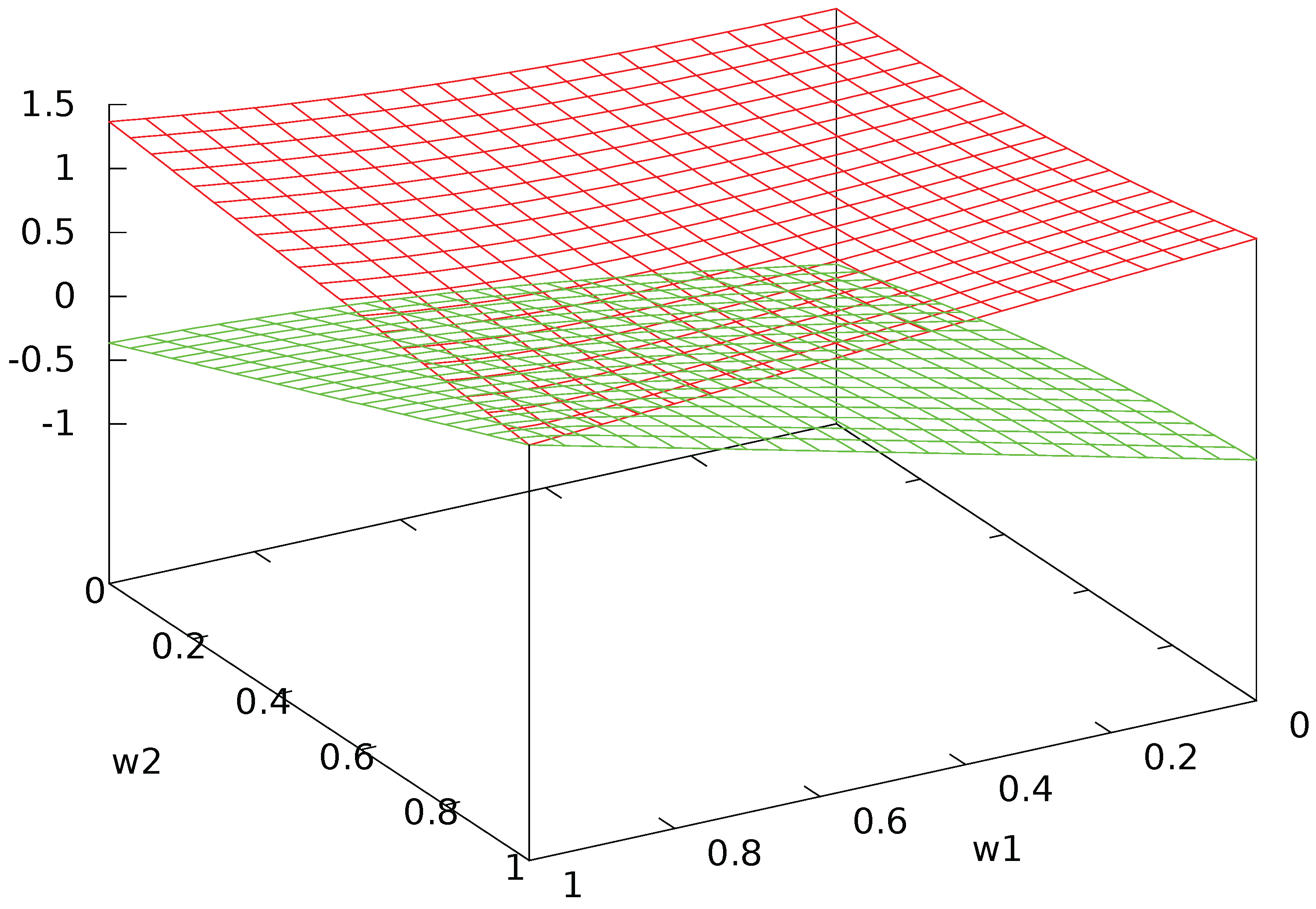
The eigenvalues are shown in Figure A1. One sees that they tend to coincide to 1 when both agents have high activity level and low interaction, while they are very much apart when interaction is high.
Figure A1.
Eigenvalues of .

Let us compute the evolution of the system by applying Schrödinger’s equation, taking the Hamiltonian to be the self-adjoint matrix , and .
represents the state of the agents at timer t. Expressed in the basis, we find, with the (reduced) Planck constant ,
and, in the standard basis, using Equation (A1):
The probability of transition from state to after time t is given by
This probability has period and maximal value . In our case, we have
which is the maximal value of the probability of transition. Its period is
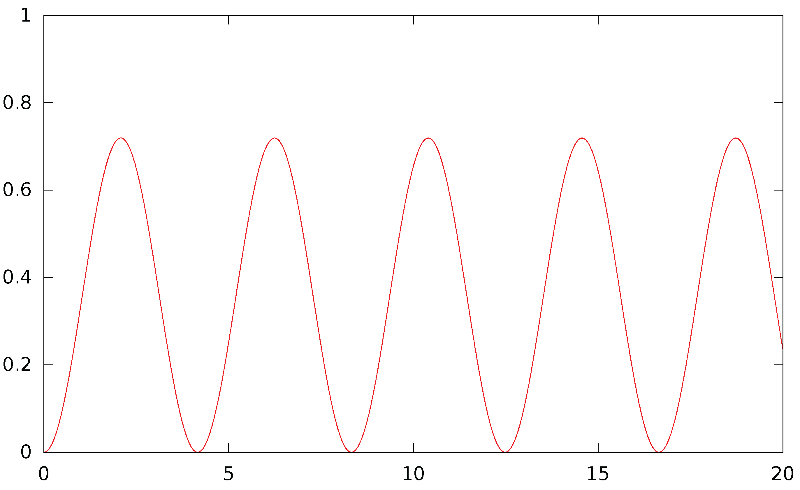
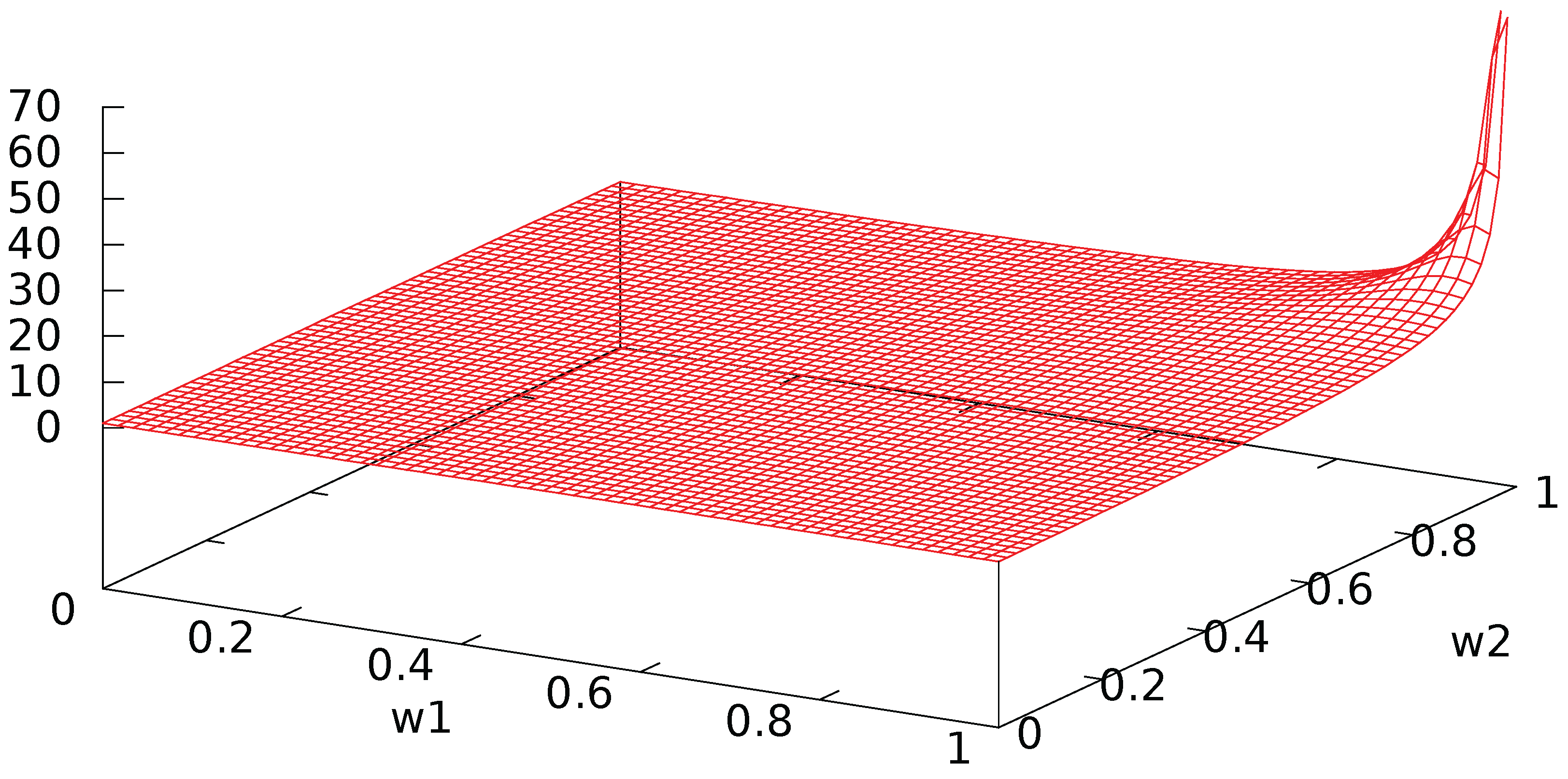
Figure A2 shows the oscillatory nature of the probability of transition. The amplitude and period of these oscillations are shown in Figure A3 and Figure A4. When both agents have a high activity level with low interaction, the period tends to infinity so that the probability of transition tends to 0: there is no evolution. Otherwise, the period is almost constant to a low value around 1 unit of time, while the amplitude is close to its maximal value when the agents have a low activity and a high interaction: clearly, interaction creates strong and rapid oscillations between the two states. In addition, the amplitude is minimal when one of the agents has no interaction while the other one has.
Figure A2.
Probability of transition from state to in unit times with , .

Figure A3.
Amplitude of probability of transition.
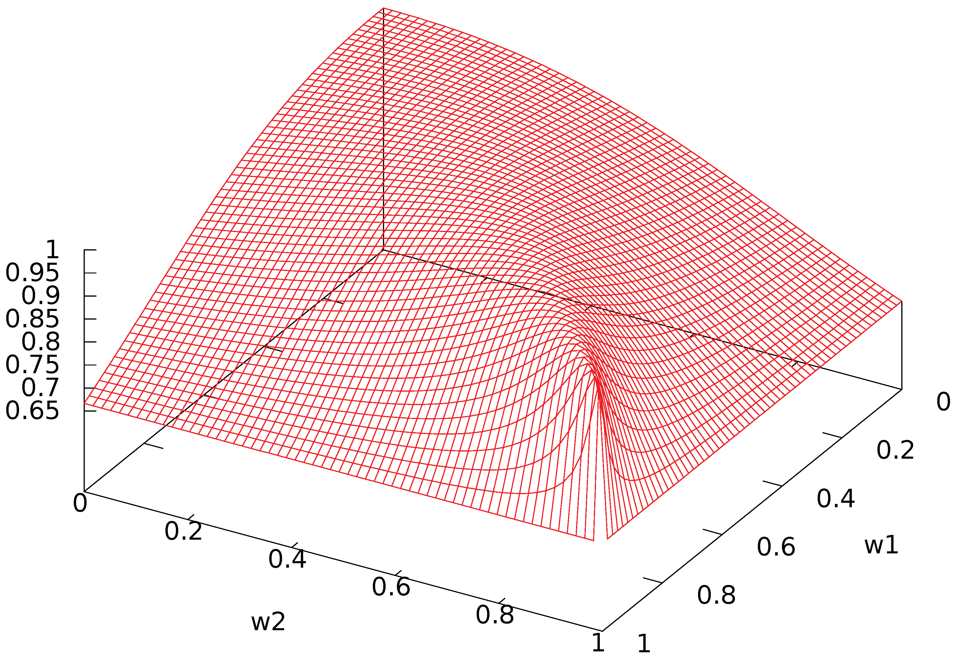
Figure A4.
Period of probability of transition in units of time.

Let us consider slightly different interaction matrices :
with . In , the antidiagonal elements are nonpositive, which, when is interpreted as an influence matrix, corresponds to an anticonformist attitude, since the agent has a tendency to adopt an opinion opposite to the one of the other agent. represents a mixed situation where agent 1 is conformist and agent 2 is anticonformist. The corresponding self-adjoint matrices are
Observe that, since in all cases the term is the same, all parameters remain the same, and only changes. Consequently, the eigenvalues and probability of transition are the same, and only the evolution of changes.
In the particular situation
the agents display no activity (or no self-confidence) and interact positively (or follow the other’s opinion fully). The eigenvalues are , and , yielding a maximal amplitude for probability transition and a period equal to . holds and the evolution is
Another extreme case is
where the two agents have negative interaction or are pure anticonformists. The eigenvalues are , and , yielding a maximal amplitude for probability transition and a period equal to . Again, holds with evolution
Note that, in both cases, the state is oscillating with maximal amplitude, which is well in line with the intuition that the opinion is very unstable in case every agent just copies the activity/opinion of the other or does exactly the opposite.
References
- Owen, G. Multilinear extensions of games. Manag. Sci. 1972, 18, 64–79. [Google Scholar] [CrossRef]
- Grabisch, M.; Roubens, M. An axiomatic approach to the concept of interaction among players in cooperative games. Int. J. Game Theory 1999, 28, 547–565. [Google Scholar] [CrossRef]
- Faigle, U.; Grabisch, M. Bases and linear transforms of TU-games and cooperation systems. Int. J. Game Theory 2016, 45, 875–892. [Google Scholar] [CrossRef]
- Penrose, R. Shadows of the Mind; Oxford University Press: Oxford, UK, 1994. [Google Scholar]
- Grabbe, J.O. An Introduction to Quantum Game Theory. arXiv 2005, arXiv:quant-ph/050621969. [Google Scholar]
- Guo, H.; Zhang, J.; Koehler, G.J. A survey of quantum games. Decis. Support Syst. 2008, 46, 318–332. [Google Scholar] [CrossRef]
- Eisert, J.; Wilkens, M.; Lewenstein, M. Quantum games and quantum strategies. Phys. Rev. Lett. 1999, 83, 3077–3080. [Google Scholar] [CrossRef]
- Vourdas, A. Comonotonicity and Choquet integrals of Hermitian operators and their applications. J. Phys. A Math. Theor. 2016, 49, 145002. [Google Scholar] [CrossRef]
- Zhang, Q.; Saad, W.; Bennis, M.; Debbah, M. Quantum Game Theory for Beam Alignment in Millimeter Wave Device-to-Device Communications. In Proceedings of the IEEE Global Communications Conference (GLOBECOM), Next Generation Networking Symposium, Washington, DC, USA, 4–8 December 2016. [Google Scholar]
- Iqbal, A.; Toor, A.H. Quantum cooperative games. Phys. Lett. A 2002, 293, 103–108. [Google Scholar] [CrossRef]
- Levy, G. Quantum game beats classical odds–Thermodynamics implications. Entropy 2017, 17, 7645–7657. [Google Scholar] [CrossRef]
- Wolpert, D.H. Information theory–The bridge connecting bounded rational game theory and statistical physics. In Complex Engineered Systems; Springer: Berlin, Germany, 2006; pp. 262–290. [Google Scholar]
- Aubin, J.-P. Cooperative fuzzy games. Math. Oper. Res. 1981, 6, 1–13. [Google Scholar] [CrossRef]
- Nielsen, M.; Chuang, I. Quantum Computation; Cambrigde University Press: Cambrigde, UK, 2000. [Google Scholar]
- Aumann, R.J.; Peleg, B. Von Neumann-Morgenstern solutions to cooperative games without side payments. Bull. Amer. Math. Soc. 1960, 66, 173–179. [Google Scholar] [CrossRef]
- Bilbao, J.M.; Fernandez, J.R.; Jiménez Losada, A.; Lebrón, E. Bicooperative games. In Cooperative Games on Combinatorial Structures; Bilbao, J.M., Ed.; Kluwer Academic Publishers: New York, NY, USA, 2000. [Google Scholar]
- Labreuche, C.; Grabisch, M. A value for bi-cooperative games. Int. J. Game Theory 2008, 37, 409–438. [Google Scholar] [CrossRef] [Green Version]
- Faigle, U.; Kern, W.; Still, G. Algorithmic Principles of Mathematical Programming; Springer: Dordrecht, the Netherlands, 2002. [Google Scholar]
- Grabisch, M.; Rusinowska, A. Influence functions, followers and command games. Games Econ. Behav. 2011, 72, 123–138. [Google Scholar] [CrossRef] [Green Version]
- Grabisch, M.; Rusinowska, A. A model of influence based on aggregation functions. Math. Soc. Sci. 2013, 66, 316–330. [Google Scholar] [CrossRef]
- Shapley, L.S. A value for n-person games. In Contributions to the Theory of Games; Kuhn, H.W., Tucker, A.W., Eds.; Princeton University Press: Princeton, NJ, USA, 1953; Volume II, pp. 307–317. [Google Scholar]
- Jackson, M.O. Social and Economic Networks; Princeton University Press: Princeton, NJ, USA, 2008. [Google Scholar]
- Hsiao, C.R.; Raghavan, T.E.S. Monotonicity and dummy free property for multi-choice games. Int. J. Game Theory 1992, 21, 301–332. [Google Scholar] [CrossRef]
- Marichal, J.-L. Weighted lattice polynomials. Discret. Math. 2009, 309, 814–820. [Google Scholar] [CrossRef]
- Rota, G.C. On the foundations of combinatorial theory I. Theory of Möbius functions. Zeitschrift für Wahrscheinlichkeitstheorie und Verwandte Gebiete 1964, 2, 340–368. [Google Scholar] [CrossRef]
- Walsh, J. A closed set of normal orthogonal functions. Am. J. Math. 1923, 45, 5–24. [Google Scholar] [CrossRef]
- Hammer, P.L.; Rudeanu, S. Boolean Methods in Operations Research and Related Areas; Springer: New York, NY, USA, 1968. [Google Scholar]
- Kalai, G. A Fourier-theoretic perspective on the Condorcet paradox and Arrow’s theorem. Adv. Appl. Math. 2002, 29, 412–426. [Google Scholar] [CrossRef]
- O’Donnell, R. Analysis of Boolean Functions; Cambridge University Press: Cambrigde, UK, 2014. [Google Scholar]
- Meyer, D.A. Quantum strategies. Phys. Rev. Lett. 1999, 82, 1052–1055. [Google Scholar] [CrossRef]
- Faigle, U.; Schönhuth, A. Asymptotic Mean Stationarity of Sources with Finite Evolution Dimension. IEEE Trans. Inf. Theory 2007, 53, 2342–2348. [Google Scholar] [CrossRef]
- Faigle, U.; Grabisch, M. Values for Markovian coalition processes. Econ. Theory 2012, 51, 505–538. [Google Scholar] [CrossRef] [Green Version]
- Bacci, G.; Lasaulce, S.; Saad, W.; Sanguinetti, L. Game Theory for Networks: A tutorial on game-theoretic tools for emerging signal processing applications. IEEE Signal Process. Mag. 2016, 33, 94–119. [Google Scholar] [CrossRef]
- Faigle, U.; Gierz, G. Markovian statistics on evolving systems. Evol. Syst. 2017. [Google Scholar] [CrossRef]
- Puterman, M. Markov Decision Processes: Discrete Stochastic Dynamic Programming; John Wiley: Hoboken, NJ, USA, 2005. [Google Scholar]
- Lozovanu, D.; Pickl, S. Optimization of Stochastic Discrete Systems and Control on Complex Networks; Springer: Cham, Switzerland, 2015. [Google Scholar]
| 1 | see also Grabisch and Roubens [2] for a general approach |
| 2 | |
| 3 | |
| 4 | Iqbal and Toor [10] discuss a 3 player situation |
| 5 | see, e.g., Levy [11] |
| 6 | cf. Wolpert [12] |
| 7 | see, e.g., Nielsen and Chang [14] |
| 8 | Non Transferable Utility game; cf. Aumann and Peleg [15] |
| 9 | |
| 10 | see also the discussion in Section 7 |
| 11 | see, e.g., [18] |
| 12 | |
| 13 | see, e.g., Jackson [22] |
| 14 | see, e.g., Penrose [4] |
| 15 | see, e.g., Nielsen and Chuang [14] |
| 16 | Hammer and Rudeanu [27] |
| 17 | |
| 18 | |
| 19 | |
| 20 |
© 2017 by the authors. Licensee MDPI, Basel, Switzerland. This article is an open access article distributed under the terms and conditions of the Creative Commons Attribution (CC BY) license (http://creativecommons.org/licenses/by/4.0/).
Share and Cite
MDPI and ACS Style
Faigle, U.; Grabisch, M. Game Theoretic Interaction and Decision: A Quantum Analysis. Games 2017, 8, 48. https://doi.org/10.3390/g8040048
AMA Style
Faigle U, Grabisch M. Game Theoretic Interaction and Decision: A Quantum Analysis. Games. 2017; 8(4):48. https://doi.org/10.3390/g8040048
Chicago/Turabian StyleFaigle, Ulrich, and Michel Grabisch. 2017. "Game Theoretic Interaction and Decision: A Quantum Analysis" Games 8, no. 4: 48. https://doi.org/10.3390/g8040048
Note that from the first issue of 2016, this journal uses article numbers instead of page numbers. See further details here.