Computing Human-Understandable Strategies: Deducing Fundamental Rules of Poker Strategy

Florida International University, School of Computing and Information Sciences; Miami, FL 33199, USA
*
Author to whom correspondence should be addressed.
Games 2017, 8(4), 49; https://doi.org/10.3390/g8040049
Submission received: 21 August 2017
/
Revised: 3 October 2017
/
Accepted: 23 October 2017
/
Published: 6 November 2017
Abstract
:Algorithms for equilibrium computation generally make no attempt to ensure that the computed strategies are understandable by humans. For instance the strategies for the strongest poker agents are represented as massive binary files. In many situations, we would like to compute strategies that can actually be implemented by humans, who may have computational limitations and may only be able to remember a small number of features or components of the strategies that have been computed. For example, a human poker player or military leader may not have access to large precomputed tables when making real-time strategic decisions. We study poker games where private information distributions can be arbitrary (i.e., players are dealt cards from different distributions, which depicts the phenomenon in large real poker games where at some points in the hand players have different distribution of hand strength by applying Bayes’ rule given the history of play in the hand thus far). We create a large training set of game instances and solutions, by randomly selecting the information probabilities, and present algorithms that learn from the training instances to perform well in games with unseen distributions. We are able to conclude several new fundamental rules about poker strategy that can be easily implemented by humans.
1. Introduction
Large-scale computation of strong game-theoretic strategies is important in many domains. For example, there has been significant recent study on solving game-theoretic problems in national security from which real deployed systems have been built, such as a randomized security check system for airports [1]. Typically large-scale equilibrium-finding algorithms output massive strategy files (which are often encoded in binary), which are stored in a table and looked up by a computer during gameplay. For example, creators of the optimal strategy for two-player limit Texas hold’em recently wrote, “Overall, we require less than 11 TB [terabytes] of storage to store the regrets and 6 TB to store the average strategy during the computation, which is distributed across a cluster of computation nodes. This amount is infeasible to store in main memory,...” [2]. While such approaches lead to very strong computer agents, it is difficult to see how a human could implement these strategies. For cases where humans will be making real-time decisions we would like to compute strategies that are easily interpretable. In essence, we are saying that a strategy is human understandable if a human could implement it efficiently in real time having memorized only a small number of items in advance.
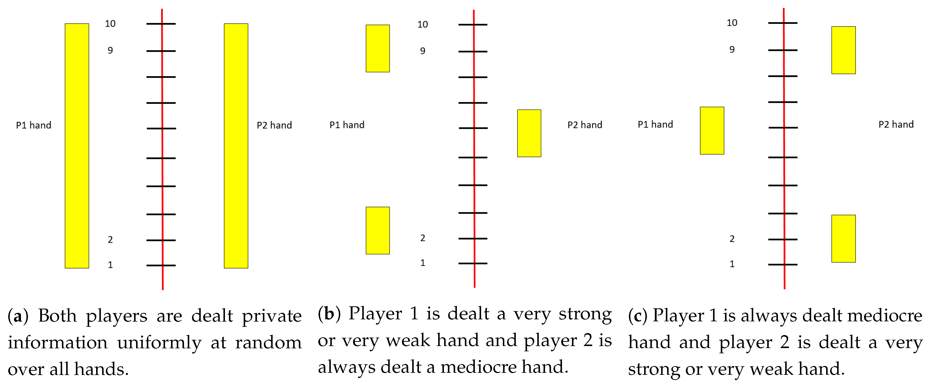
Suppose a human plans to play the following two-player no-limit poker game. Player 1 and player 2 both ante $0.50 and are dealt a card from a 10-card deck and each have a stack of $3 after posting the ante. Player 1 can bet any multiple of 0.1 from 0 to 3 (he has 31 possible actions for each hand). Player 2 can then call or fold. If player 2 folds, then player 1 wins the $1 from the antes. Otherwise the player with the better card wins the amount bet plus the antes. For example, if player 1 has a 4, player 2 has a 9, player 1 bets 0.4 and player 2 calls, then player 2 wins 0.4 plus the antes.
If both players are dealt cards uniformly (Figure 1a), then a Nash equilibrium strategy for player 1 is:
- Card 1: Bet 0.1 pr. 0.091, 0.6 pr. 0.266, 1.8 pr. 0.643
- Card 2: Bet 0 pr. 0.660, 0.3 pr. 0.231, 0.6 pr. 0.109
- Card 3–6: Bet 0 pr. 1
- Card 7: Bet 0.1 pr. 1
- Card 8: Bet 0.3 pr. 1
- Card 9: Bet 0.6 pr. 1
- Card 10: Bet 1.8 pr. 1
This can be computed quickly using, e.g., a linear programming formulation [3]. Note that the equilibrium strategy includes bluffing (i.e., betting with weak hands).
However, suppose the cards are dealt according a different distribution: player 1 is either dealt a very strong hand (10) or a very weak hand (1) with probability 0.5 while player 2 is always dealt a medium-strength hand (Figure 1b). Then the equilibrium strategy for player 1 is:
- Card 1: Bet 0 pr. 0.25, 3 pr. 0.75
- Card 10: Bet 3 pr. 1
If player 1 is always dealt a medium-strength hand (5) while player 2 is dealt a very strong or very weak hand with probability 0.5 (Figure 1c), then the equilibrium strategy is:
- Card 5: Bet 0 pr. 1
What if player 1 is dealt a 1 with probability 0.09, 2 with probability 0.19, 3 with probability 0.14, etc.? For each game instance induced by a probability distribution over the private information, we could solve it quickly if we had access to a linear programming (LP) solver. But what if a human is to play the game without knowing the distribution in advance and without aid of a computer? He would need to construct a strong game plan in advance that is capable of playing well for a variety of distributions with minimal real-time computation. A natural approach would be to solve and memorize solutions for several games in advance, then quickly determine which of these games is closest to the one actually encountered in real time. This is akin to the k-nearest neighbors (k-nn) algorithm from machine learning. A second would be to construct understandable rules (e.g., if .. else ..) from a database of solutions that can be applied to a new game. This is akin to the decision tree and decision list approaches. Thus, we are proposing to apply approaches from machine learning in order to improve human ability to implement Nash equilibrium strategies. Typically algorithms from machine learning have been applied to game-theoretic agents only in the context of learning to exploit mistakes of suboptimal opponents (aka opponent exploitation). By and large the approaches for computing Nash equilibrium and opponent exploitation have been radically different. We provide a new perspective here by integrating learning into the equilibrium-finding paradigm.
We present a novel learning formulation of this problem. In order to apply algorithms we develop novel distance functions (both between pairs of input points and between pairs of output points) which are more natural for our setting than standard distance metrics. To evaluate our approaches we compute a large database of game solutions for random private information distributions. We are able to efficiently apply k-nn to the dataset using our custom distance functions. We observed that we are able to obtain low testing error even when training on a relatively small fraction of the data, which suggests that it is possible for humans to learn strong strategies by memorizing solutions to a carefully selected small set of presolved games. However, this approach would require humans to quickly be able to compute the distance between a new game and all games from the training database in order to determine the closest neighbor, which could be computationally taxing. Furthermore, there are some concerns as to whether this would actually constitute “understanding” as opposed to “memorizing”. Thus, we focus on the decision tree approach, which allows us to deduce simple human-understandable rules that can be easily implemented.
While prior approaches for learning in games of imperfect information (and poker specifically) often utilize many domain-specific features (e.g., number of possible draws to a flush, number of high cards on the board, etc.), we prefer to develop approaches that are do not require knowing expert domain features (since they are likely not relevant for other domains and, in the case of poker, may not be relevant even for other seemingly similar variants). The features we use are the cumulative distribution function values of the private information states of the players, which are based purely on the rules of the game. (We also compare performance of using several other representations, e.g., using pdf values, and separating out the data for each hand to create 10 data points per game instance instead of 1). Thus, the approach is general and not reliant on expert poker knowledge.
2. Qualitative Models and Endgame Solving
There has been some prior study of human understandable strategies in imperfect-information games, and in poker specifically. Ankenman and Chen compute analytical solutions of several simplified poker variants by first assuming a given human-understandable qualitative structure on the equilibrium strategies, and then computing equilibrium strategies given this presumed structure, typically by solving a series of indifference equations [9]. While the computed strategies are generally interpretable by humans, the models were typically constructed from a combination of trial and error and expert intuition, and not constructed algorithmically. More recent work has shown that leveraging such qualitative models can lead to new equilibrium-finding algorithms that outperform existing approaches [10]. That work proposed three different qualitative models for the final round of two-player limit Texas hold’em (Figure 2), and showed empirically that equilibrium strategies conformed to one of the models for all input information distributions (and that all three were needed). Again here the models were constructed by manual trial and error, not algorithmically.
We note that while the problem we are considering in this paper is a “toy game”, it captures important aspects of real poker games and we expect our approaches to have application to larger more realistic variants (our game generalizes many common testbed variants; if we had allowed player 2 to bet after player 1 checks and the deck had only 3 cards and only one bet size is allowed, this would be Kuhn poker). In the recent Brains vs. Artificial Intelligence two-player no-limit Texas hold’em competition, the agent Claudico computed the strategy for the final betting round in real time, and the best human player in the world for that variant (Doug Polk) commented that the “endgame solver” was the strongest component of the agent [11], and endgame solving was also a crucial component of subsequent success of the improved agent Libratus [12]. The creator of another recent superhuman agent has stated that “DeepStack is all endgame solving,” referring to the fact that its algorithm works by viewing different rounds of the game as separate endgames which are solved independently, using deep learning to estimate the values of the endgames terminal states [13]. Endgame solving assumes that both agents had private information distributions induced by the strategies for the prior rounds using Bayes’ rule, assuming they had been following the agent’s strategy for the prior rounds [14]. The game we study here is very similar to no-limit Texas hold’em endgames, except that we are assuming a ten-card deck, specific stack sizes and betting increment, and that raises are not allowed. We expect our analysis to extend in all of these dimensions and that our approaches will have implications for no-limit Texas hold’em. No-limit Texas hold’em is the most popular poker variant for humans, and is a widely recognized AI challenge problem. The game tree has approximately states for the variant played in the Computer Poker Competition [15]. There has been significant interest in endgame solving in particular in the last several years [12,13,16,17].
3. Learning Formulation
We now describe how we formulate the problem of computing a solution to a new game instance from a database of solutions to previously solved game instances as a learning problem. The inputs will be the 20 values of the private information cumulative distribution function (cdf). First are the ten values for player 1 (the probability he is dealt ≤ 1, probability he is dealt ≤ 2, etc.), followed by the ten cdf values for player 2. For example for the uniform case the input would be
for the situation where player 1 is dealt a 10 or 1 with prob. 0.5 and player 2 is always dealt a 5 it is
and for the situation where player 1 is always dealt a 5 and player 2 is dealt a 10 or 1 with prob. 0.5
The output will be a vector of the 310 Nash equilibrium strategy probabilities of betting each size with each hand. First for betting 0, 0.1, 0.2, …, 3 with 1, then with 2, etc. (recall that there are 31 sizes for each of ten hands). For example for the uniform case the output would be
We could have created ten different data points for each game corresponding to the strategy for each hand, as opposed to predicting the full strategy for all hands; however we expect that predicting complete strategies is better than just predicting strategies for individual hands because the individual predicted hand strategies may not balance appropriately and could be highly exploitable as a result. We will explore this design choice in the experiments in Section 4.
To perform learning on this formulation, we need to select a distance function to use between a pair of inputs as well as a distance (i.e., cost) between each pair of outputs. Standard metrics of Euclidean or Manhattan distance are not very appropriate for probability distributions. A more natural and successful distance metric for this setting is earth mover’s distance (EMD). While early approaches for computing groupings of hands used L2 [18], EMD has been shown to significantly outperform other approaches, and the strongest current approaches for game abstraction use EMD [19]. Informally, EMD is the “minimum cost of turning one pile into the other, where the cost is assumed to be amount of dirt moved times the distance by which it is moved”, and there exists a linear-time algorithm for computing it for one-dimensional histograms (Figure 3).
We define a new distance metric for our setting that generalizes EMD to multiple distributions. Suppose we want to compute the distance between training input vector X and testing input vector . Each vector contains 20 probabilities, 10 corresponding to player 1’s distribution and 10 to player 2’s. Our distance function will compute the EMD separately for each player, then return the average (Algorithm 1). We note that before the aggregation we normalize the EMD values by the maximum possible value (the distance between a point mass on the left-most and right-most columns) to ensure that the maximum of each is 1. We also create a new distance (i.e., cost) function between predicted output vector and the actual output vector from the training data Y (the output vectors have length 310, corresponding to 31 bet sizes for 10 hands). It computes EMD separately for the strategy vectors of size 31 for each hand which are then normalized and averaged (Algorithm 2). After specifying the form of the inputs and outputs and a distance metric between each pair of inputs and outputs, we have formulated the problem as a machine learning problem.
Note that our learning algorithms can take any cost function between output vectors as input. In addition to our generalized EMD metric, we can also compute exact exploitability. In two-player zero-sum games, the exploitability of a strategy for player i is the difference between the game value to player i and the expected payoff of against a nemesis strategy for the opponent. This is a good measure of the performance; all Nash equilibrium strategies have zero exploitability, and strategies with high exploitabilty can perform very poorly against a strong opponent. In general there exists a general linear program formulation for computing the best response payoff to a strategy (from which one can then subtract the game value to obtain exploitability) [3]. However, we would like to avoid having to do a full linear program solve each time that a cost computation is performed during the run of a learning algorithm. There also exists a more efficient linear-time (in the size of the full game tree) algorithm called expectimax for computing best responses (and consequently exploitability as well) for two-player zero-sum games [20]. For our specific setting (where both players are dealt a single card from a distribution and then select a single bet size from a discrete space), it turns out that we can obtain exploitability even faster by applying the technique described in Algorithm 3. This algorithm iterates over all bet sizes and for each, determines whether player 2 would prefer to call or fold against the given strategy of player 1 (depending on how often player 1 is betting with a worse vs. better hand in relation to the size of the pot). The key observation is that if player 2 calls, then he will win (betSize + 1) whenever player 1 has a worse hand, and he will lose betSize when player 1 has a better hand. So his expected payoff of calling will be
Since the expected payoff of folding is 0, he will prefer to call if
which yields the equation used in the algorithm.
| Algorithm 1 Distance between input vectors X, |
| Inputs: cdf vectors , number of players n, deck size d ← cdf-to-pdf(X) ← cdf-to-pdf() resultTotal ← 0 for to do start ← end ← start + d result ← 0 for start to end−1 do + result ← result + result ← result / (d−1) resultTotal ← resultTotal + result return (resultTotal / n) |
| Algorithm 2 Distance between output vectors Y, |
| Inputs: Strategy vectors , deck size d, number of bet sizes b resultTotal ← 0 for to do start end ← start + b result ← 0 for start to end-1 do + result ← result + result ← result / (b-1) resultTotal ← resultTotal + result return (resultTotal / d) |
| Algorithm 3 Compute exploitability |
| Inputs: is probability P1 is dealt card i and P2 is dealt card j, is probability that P1 bets the bet size with card i, is the bet size, is the game value to player 1 numCards numBets for to numCards do for to numBets do betSize probWorse probBetter for to do probWorse ← probWorse + probs[j][i] · strategy[j][b] for to numCards do probBetter ← probBetter + probs[j][i] · strategy[j][b] sum ← probWorse + probBetter if then return () |
4. Experiments
We constructed a database of 100,000 game instances by generating random hand distributions and then computing a Nash equilibrium using the linear program formulation with Gurobi’s solver [21]. The naïve approach for constructing the distributions (of assigning uniform distributions for the players independently) is incorrect because it does not account for the fact that if one player is dealt a card then the other player cannot also be dealt that card (as is the case in real poker). We instead used a Algorithm 5. We first generate the two distributions independently as in the naïve approach, using the procedure described in Algorithm 4. Algorithm 5 then multiplies these individual probabilities together only for situations where players are dealt different cards to compute a joint distribution.
| Algorithm 4 Generate point uniformly at random from n-dimensional simplex |
| Inputs: dimension n for to do randomDouble(0,1) for to do return a |
| Algorithm 5 Generate private information distribution |
| Inputs: dimension n, independent distributions for to do for to do if i != j then next next next for to do for to do return |
We experimented with several data representations. The second uses the pdf values as the 20 features instead of the cdfs. The third separates each datapoint into 10 different points, one for each hand of player 1. Here the first 20 inputs are the cdfs as before, followed by a card number (1–10), which can be viewed as an additional 21st input, followed by the 31 strategy probabilities for that card. The fourth uses this approach with the pdf features. The 5th and 6th approaches are similar, but for the 21st input they list the cdf value of the card, not the card itself. The 7th–10th are similar to the 3rd–6th, but randomly sample a single bet size from the strategy vector to use as the output.
We created decision trees using 80,000 of the games from the database, using the standard division of 80% of the data for training and 20% for testing (so we trained on 64,000 games and tested on 16,000). We used Python’s built in decision tree regressor function from sklearn.tree from the scikit-learn library, which we were able to integrate with our new distance metrics. We constructed the optimal decision tree for depth ranging from 3 up to 20. From Figure 4a, we can see the errors of the optimal tree as a function of the depth, for each of the different data representations. Not surprisingly error decreases monotonically with depth; however, increasing the depth leads to an exponential increase in the number of nodes. Figure 4b shows how error decreases as a function of the (log of the) the number of nodes in the optimal decision tree.
The fourth representation, which uses the pdf values plus the cdf value of the card as the inputs, produces lowest error, and in general the approaches that output the data separately for each card produce lower errors than the ones that output full 310-length vectors. Note that if we were using full exploitability to evaluate the strategies produced then almost surely using the full 310 outputs would perform better, since they will take into account aggregate strategies across all hands to ensure the overall strategy is balanced; if we bet one size with a weak hand and a different size with a strong hand, it would be very easy for the opponent to exploit us. In fact, for other machine learning approaches, such as k-nn, using the full 310 outputs performs better; but for decision trees using separate outputs for each hand leads to better branching rules which produces lower error. Note that the pdf features encode more information than the cdfs (it is possible for two games with the same cdfs to have different pdfs), so we would expect pdf features to generally outperform cdf features.
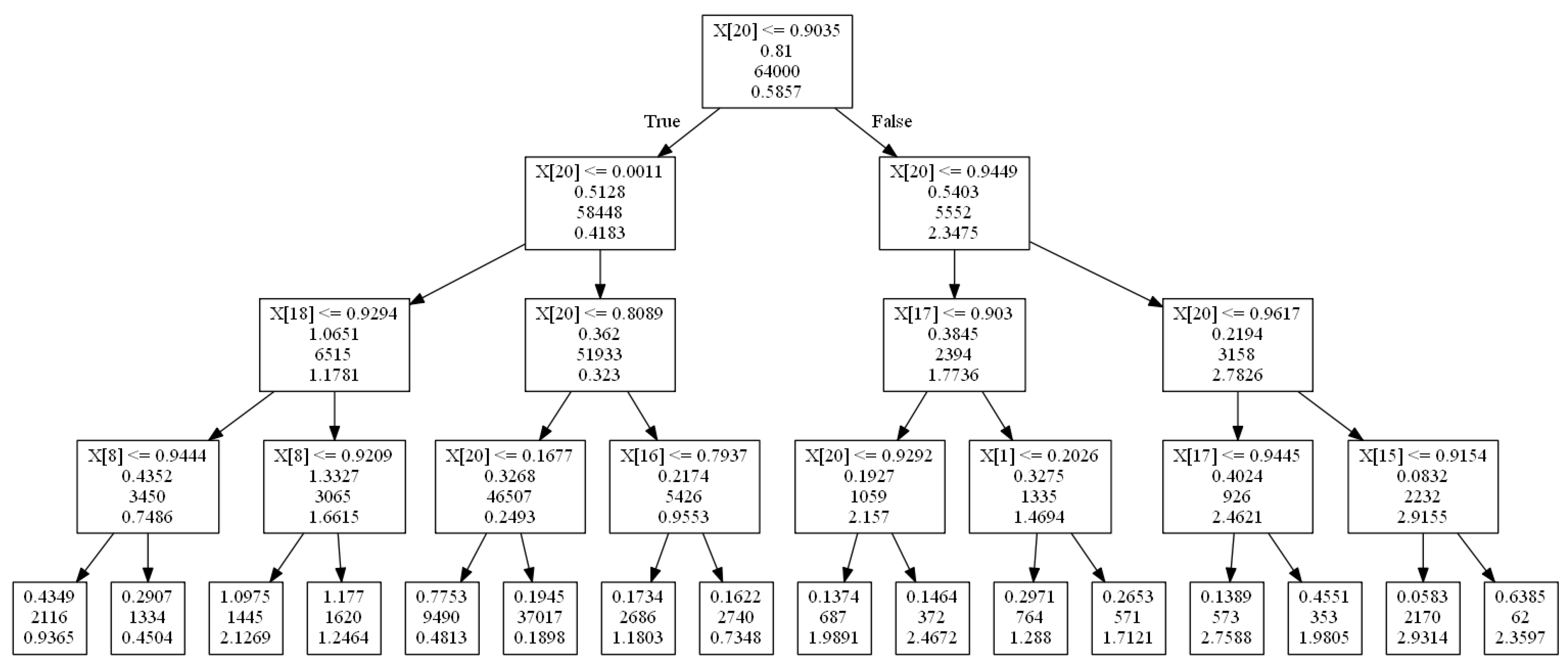
The optimal depth-4 decision tree for cdf input values, cdf value for a single card, and predicts a single bet size, is shown in Figure 5. At each node the left edge corresponds to the True branch and the right to the False branch. The node entries are the variable/value branched on, the error induced due to the current branch split, the sample for the current split, and the output (i.e., bet size) predicted (leaf nodes only contain the final three). For example, the far right leaf node says that if is false (i.e., player 1 has a hand with cdf value ), ..., if is false (i.e., the cdf value of a card 6 for player 2 is ), then output a bet size of 2.3597.
From the optimal tree, we can deduce several fundamental rules of poker strategy. The “80-20 Rule” is based on the branch leading to the very small bet size of 0.1898, and the “All-in Rule” is based on the branch leading to the large bet size of 2.9314 on the far right of the tree.
Fundamental Rule of Poker Strategy 1 (80-20 Rule).
If your hand beats between 20% and 80% of the opponent’s hand distribution, then you should always check (or make an extremely small bet).
Fundamental Rule of Poker Strategy 2 (All-In Rule).
If your hand beats 95% of the opponent’s distribution of hands, and furthermore the opponent’s distribution contains a weak or mediocre hand no more than 90% of the time (i.e., it contains at least 10% strong hands), then you should go all-in.
Prior “fundamental rules” have been proposed, but often these are based on psychological factors or personal anecdotes, as opposed to rigorous analysis. For example, Phil Gordon writes, “Limping1 is for Losers. This is the most important fundamental in poker—for every game, for every tournament, every stake: If you are the first player to voluntarily commit chips to the pot, open for a raise. Limping is inevitably a losing play. If you see a person at the table limping, you can be fairly sure he is a bad player. Bottom line: If your hand is worth playing, it is worth raising” [22]. However, some very strong agents such as Claudico [11] and Libratus [12] actually employ limping sometimes (in fact the name Claudico is Latin for “I limp”).
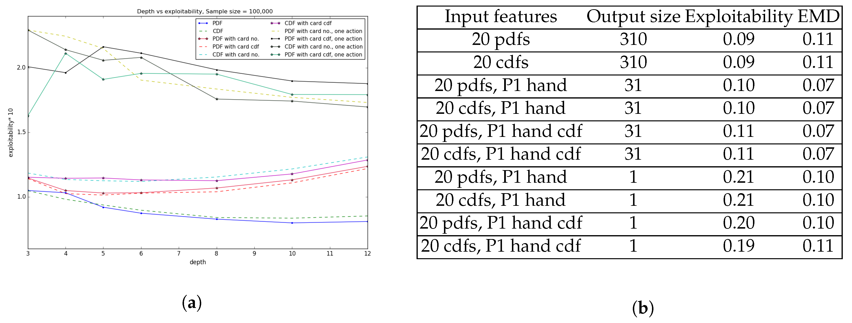
We also performed experiments using the exploitability cost function from Algorithm 3. For the first representation with 10 pdf values for both player’s each possible hand, joint probability distribution was calculated as above. The output strategy vector of the 31 bet sizes for each hand for player 1 was derived from the decision tree model. Then according to Algorithm 3 best response payoff for player 1 was calculated and subtracted from the presolved game value. For all the other representations with individual hand for player 1 as the 21th input feature, decision tree output was extracted for each card individually and then was combined into a single output strategy vector.
Figure 6a depicts the change in exploitability with respect to the depth of the decision tree. 310 output strategy outperforms 31 output vector strategy by a small margin whereas output with just the bet size in the last four representation produces relatively higher exploitability compared to the previous six comprehensive representations. Also later representations with just single bet size doesn’t result in smooth transition over depth for lower values due to the approximation in probability calculation considering only the most probable bet size, where there might exist other bet sizes for that particular hand with relatively smaller but positive probability. The table in Figure 6b shows exploitability and EMD error among the different representations with depth of the tree limited to 5. It is evident from the experimental result that all the representations produce relatively negligible EMD error and exhibit low exploitability, i.e., in the range 0.09–0.21 as the maximum possible exploitability is the highest bet value of 3. The last four representations with single bet value over each individual hand are more prone to exploitability as expected since the probability of betting the other 30 possible values are totally ignored. Third to sixth entry of the table with 20 pdf and cdf representation along with player 1’s individual hand, where the output strategy is the 31 probability distribution over each bet size of that particular hand, best optimizes the tradeoff between exploitability and interpretability.
5. Conclusions
We presented a novel formulation of the problem of computing strong game-theoretic strategies that are human understandable as a machine learning problem. Traditionally computing strong strategies in games has fallen under the domain of specialized equilibrium-finding algorithms that produce massive strategy files which are unintelligible to humans. We used private information cdf values as the input features and the strategy probability vectors as the outputs, and devised novel distance functions between pairs of inputs and outputs. We also provided a novel procedure for generating random distributions of private information, which we used to create a large database of game solutions. We created algorithms that compute strategies that can be easily implemented by humans, and deduced several new fundamental rules about poker strategy. We note that the contributions are not specific to poker games. The model and formulation would apply to any multiplayer imperfect-information game where agents are given ordered private information signals. The approaches could also apply to perfect-information games where we can generate a database of games by modifying the values of natural parameters. The approaches are also not specific to two-player zero-sum games, though they do assume that solutions can be computed for the games used in training, which can be more challenging for other game classes. We would like to further evaluate our new distance metrics. An effective distance metric between strategies would have many potential applications. For instance, a recent algorithm for opponent exploitation computed the “closest” strategy to a given prior strategy that agreed with the observations, using several different distance metrics [23]. Effective strategy distance metrics would also be useful for detecting “bot” agents on online sites who are playing a strategy similar to a specific known strategy.
Acknowledgments
Initial work for this project was done by the primary author as self-funded independent research. The latter phase was performed while both authors were at the School of Computing and Information Sciences at Florida International University, funded by the start-up package of the primary author. This project is not supported by any grants.
Author Contributions
Sam Ganzfried conceived the idea and model, wrote the majority of the paper, created several of the figures, devised the algorithms, created the database of game solutions, and devised the fundamental rules of poker strategy described in Section 4. Farzana Yusuf designed and performed the experiments described in Section 4, created Figure 4, Figure 5 and Figure 6, and wrote the experimental results in Section 4.
Conflicts of Interest
The authors declare no conflict of interest.
References
- Paruchuri, P.; Pearce, J.P.; Marecki, J.; Tambe, M.; Ordonez, F.; Kraus, S. Playing games with security: An efficient exact algorithm for Bayesian Stackelberg Games. In Proceedings of the International Conference on Autonomous Agents and Multi-Agent Systems (AAMAS), Estoril, Portugal, 12–16 May 2008. [Google Scholar]
- Bowling, M.; Burch, N.; Johanson, M.; Tammelin, O. Heads-up Limit Hold’em Poker is Solved. Science 2015, 347, 145–149. [Google Scholar] [CrossRef] [PubMed]
- Koller, D.; Megiddo, N. The Complexity of Two-Person Zero-Sum Games in Extensive Form. Games Econ. Behav. 1992, 4, 528–552. [Google Scholar] [CrossRef]
- Bertsimas, D.; Chang, A.; Rudin, C. Ordered Rules for Classification: A Discrete Optimization Approach to Associative Classification; Operations Research Center Working Paper Series OR 386-11; Massachusetts Institute of Technology, Operations Research Center: Cambridge, MA, USA, 2011. [Google Scholar]
- Jung, J.; Concannon, C.; Shroff, R.; Goel, S.; Goldstein, D.G. Simple rules for complex decisions. arXiv, 2017; arXiv:1702.04690. [Google Scholar] [CrossRef]
- Lakkaraju, H.; Bach, S.H.; Leskovec, J. Interpretable decision sets: A joint framework for description and prediction. In Proceedings of the 22nd ACM SIGKDD International Conference on Knowledge Discovery and Data Mining, San Francisco, CA, USA, 13–17 August 2016. [Google Scholar]
- Letham, B.; Rudin, C.; McCormick, T.H.; Madigan, D. Interpretable classifiers using rules and Bayesian analysis: Building a better stroke prediction model. Ann. Appl. Stat. 2015, 9, 1350–1371. [Google Scholar] [CrossRef]
- Marewski, J.N.; Gigerenzer, G. Heuristic decision making in medicine. Dialogues Clin. Neurosci. 2012, 14, 77–89. [Google Scholar] [PubMed]
- Ankenman, J.; Chen, B. The Mathematics of Poker; ConJelCo LLC: Pittsburgh, PA, USA, 2006. [Google Scholar]
- Ganzfried, S.; Sandholm, T. Computing equilibria by incorporating qualitative models. In Proceedings of the International Conference on Autonomous Agents and Multi-Agent Systems (AAMAS), Toronto, ON, Canada, 10–14 May 2010. [Google Scholar]
- Ganzfried, S. Reflections on the First Man vs. Machine No-Limit Texas Hold ’em Competition. ACM SIGecom Exch. 2015, 14, 2–15. [Google Scholar] [CrossRef]
- Brown, N.; Sandholm, T. Safe and Nested Endgame Solving in Imperfect-Information Games. In Proceedings of the TheWorkshops of the Thirty-First AAAI Conference on Artificial Intelligence (AAAI-17), San Francisco, CA, USA, 4–5 February 2017. [Google Scholar]
- Moravcík, M.; Schmid, M.; Burch, N.; Lisý, V.; Morrill, D.; Bard, N.; Davis, T.; Waugh, K.; Johanson, M.; Bowling, M.H. DeepStack: Expert-Level Artificial Intelligence in No-Limit Poker. arXiv, 2017; arXiv:1701.01724. [Google Scholar]
- Ganzfried, S.; Sandholm, T. Endgame Solving in Large Imperfect-Information Games. In Proceedings of the International Conference on Autonomous Agents and Multi-Agent Systems (AAMAS), Istanbul, Turkey, 4–8 May 2015. [Google Scholar]
- Johanson, M. Measuring the Size of Large No-Limit Poker Games; Technical Report; University of Alberta: Edmonton, AB, Canada, 2013. [Google Scholar]
- Burch, N.; Johanson, M.; Bowling, M. Solving Imperfect Information Games Using Decomposition. In Proceedings of the AAAI Conference on Artificial Intelligence (AAAI), Québec City, QC, Canada, 27–31 July 2014. [Google Scholar]
- Moravcik, M.; Schmid, M.; Ha, K.; Hladik, M.; Gaukrodger, S.J. Solving Imperfect Information Games Using Decomposition. In Proceedings of the AAAI Conference on Artificial Intelligence (AAAI), Phoenix, AZ, USA, 12–17 February 2016. [Google Scholar]
- Gilpin, A.; Sandholm, T.; Sørensen, T.B. Potential-Aware Automated Abstraction of Sequential Games, and Holistic Equilibrium Analysis of Texas Hold’em Poker. In Proceedings of the AAAI Conference on Artificial Intelligence (AAAI), Vancouver, BC, Canada, 22–26 July 2007. [Google Scholar]
- Johanson, M.; Burch, N.; Valenzano, R.; Bowling, M. Evaluating State-Space Abstractions in Extensive-Form Games. In Proceedings of the International Conference on Autonomous Agents and Multi-Agent Systems (AAMAS), Saint Paul, MN, USA, 6–10 May 2013. [Google Scholar]
- Michie, D. Game-playing and game-learning automata. In Advances in Programming and Non-Numerical Computation; Fox, L., Ed.; Pergamon: New York, NY, 1966; pp. 183–200. [Google Scholar]
- Gurobi Optimization, Inc. Gurobi Optimizer Reference Manual; Version 6.0; Gurobi Optimization, Inc.: Houston, TX, USA, 2014. [Google Scholar]
- Gordon, P. Phil Gordon’s Little Gold Book: Advanced Lessons for Mastering Poker 2.0; Gallery Books: New York, NY, USA, 2011. [Google Scholar]
- Ganzfried, S.; Sandholm, T. Game theory-based opponent modeling in large imperfect-information games. In Proceedings of the International Conference on Autonomous Agents and Multi-Agent Systems (AAMAS), Taipei, Taiwan, 2–6 May 2011. [Google Scholar]
| 1 | In poker a “limp” is a play when one player only matches the antes in the first play as opposed to betting. |
Figure 1.
Three example hand distributions defining simplified poker games. The Y-axis is the hand, from 1 (worst possible hand) to 10 (best possible). For each figure, the boxes on the left denote player 1’s distribution of hands, and the boxes on the right denote player 2’s hand distribution.
Figure 1.
Three example hand distributions defining simplified poker games. The Y-axis is the hand, from 1 (worst possible hand) to 10 (best possible). For each figure, the boxes on the left denote player 1’s distribution of hands, and the boxes on the right denote player 2’s hand distribution.

Figure 2.
Three qualitative models for two-player limit Texas hold’em river endgame play.
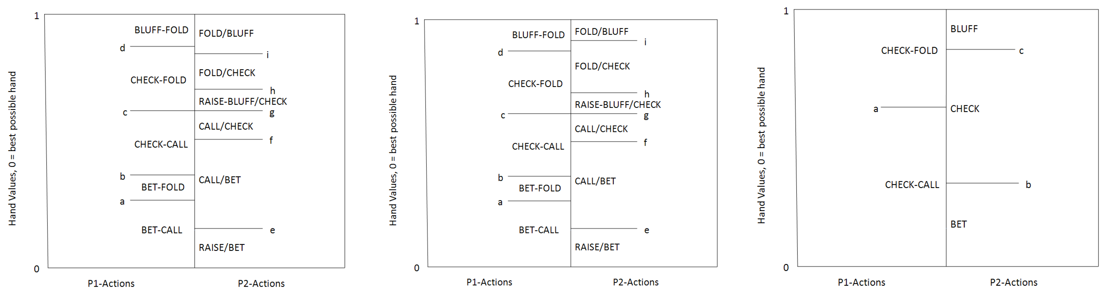
Figure 3.
Earth-mover’s distance has proven a successful metric for distance between probability distributions.
Figure 3.
Earth-mover’s distance has proven a successful metric for distance between probability distributions.

Figure 4.
Depth vs. #nodes and error; error curves are decreasing in depth, #nodes are increasing (Figure 4a). Number of nodes vs. error in decision tree (Figure 4b).
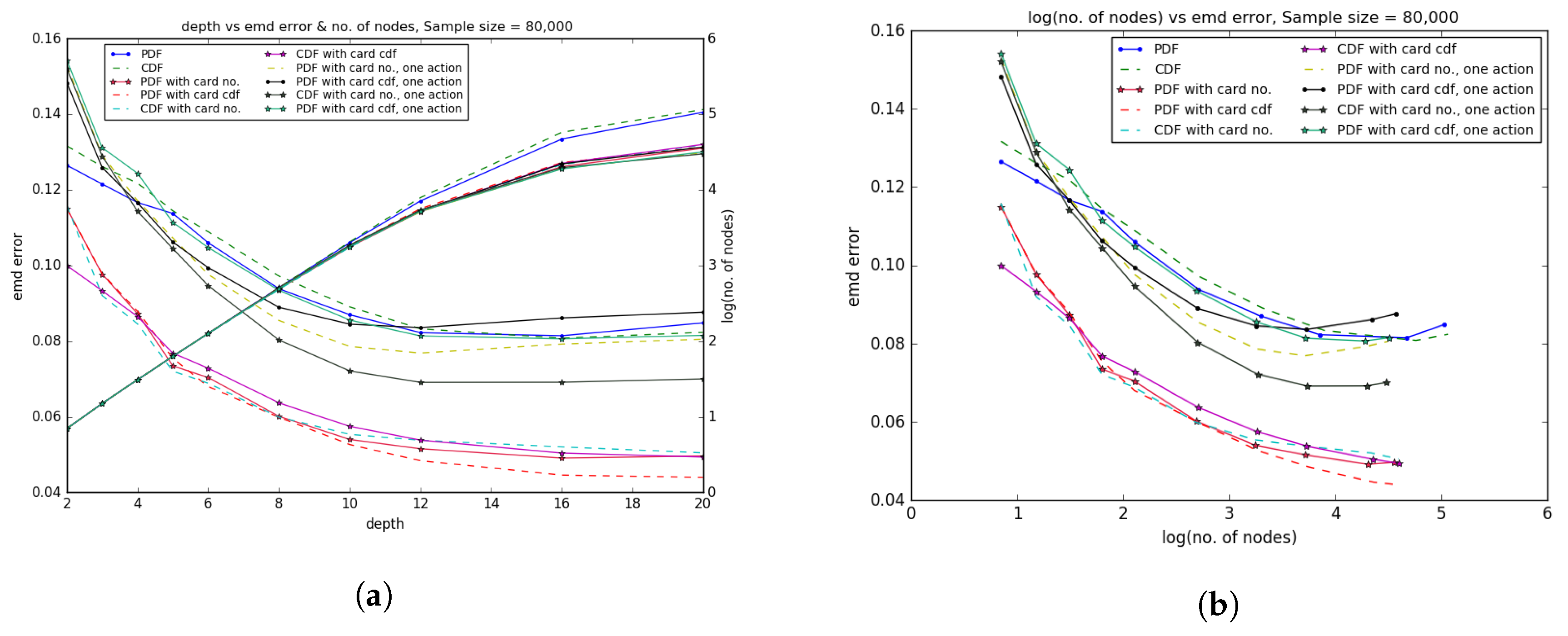
Figure 5.
Rules for optimal depth-4 decision tree.
© 2017 by the authors. Licensee MDPI, Basel, Switzerland. This article is an open access article distributed under the terms and conditions of the Creative Commons Attribution (CC BY) license (http://creativecommons.org/licenses/by/4.0/).
Share and Cite
MDPI and ACS Style
Ganzfried, S.; Yusuf, F. Computing Human-Understandable Strategies: Deducing Fundamental Rules of Poker Strategy. Games 2017, 8, 49. https://doi.org/10.3390/g8040049
AMA Style
Ganzfried S, Yusuf F. Computing Human-Understandable Strategies: Deducing Fundamental Rules of Poker Strategy. Games. 2017; 8(4):49. https://doi.org/10.3390/g8040049
Chicago/Turabian StyleGanzfried, Sam, and Farzana Yusuf. 2017. "Computing Human-Understandable Strategies: Deducing Fundamental Rules of Poker Strategy" Games 8, no. 4: 49. https://doi.org/10.3390/g8040049
Note that from the first issue of 2016, this journal uses article numbers instead of page numbers. See further details here.