Game of Thrones: Accommodating Monetary Policies in a Monetary Union

Abstract

In this paper, we present an application of the dynamic tracking games framework to a monetary union. We use a small stylized nonlinear three-country macroeconomic model of a monetary union to analyze the interactions between fiscal (governments) and monetary (common central bank) policy makers, assuming different objective functions of these decision makers. Using the OPTGAME algorithm, we calculate solutions for several games: a noncooperative solution where each government and the central bank play against each other (a feedback Nash equilibrium solution), a fully-cooperative solution with all players following a joint course of action (a Pareto optimal solution) and three solutions where various coalitions (subsets of the players) play against coalitions of the other players in a noncooperative way. It turns out that the fully-cooperative solution yields the best results, the noncooperative solution fares worst and the coalition games lie in between, with a broad coalition of the fiscally more responsible countries and the central bank against the less thrifty countries coming closest to the Pareto optimum.

1. Introduction

The Great Recession, the financial and economic crisis of 2007–2010, was the most severe contraction of advanced economies since the Great Depression of the 1930s. Fiscal policy makers reacted to this event with expansionary policies, both through discretionary measures and automatic stabilizers, even though many countries already entered the crisis with high public debt and deficits. This policy contributed to diminishing the negative effects of the crisis on output and employment, but exacerbated the already tense situation in public finances for many countries. Monetary policy mostly accommodated the expansionary course of action by governments, leading to unprecedentedly low levels of interest rates in the developed economies. It is now widely agreed that this accommodating monetary policy, together with fiscal expansion during the early phase of the Great Recession, prevented it from developing into a disaster like the Great Depression. In the meantime, economic growth after the crisis returned to previous rates in most industrialized countries, and their economies are seen to be on a path towards firm growth by now.

However, some special problems are present in the European Union, and the Euro Area in particular. Especially in the southern countries, policy makers are still struggling with high unemployment, low or negative growth and a lack of economic dynamics similar to the “eurosclerosis” of the 1970s and 1980s. One reason for this adverse development can be seen in the heterogeneity of the Euro Area’s state of economic development, combined with unfavorable effects of the “one size fits all” monetary union. Monetary policy, and exchange rate policy in particular, is no longer available as an instrument to national policy makers in the Euro Area, and internal depreciation in an economically-weak country like Greece does not seem to be a viable option. This leads to pressure on the European Central Bank from different forces, with some governments asking for a more relaxed monetary policy to accommodate their expansionary budgetary policies and others pressing for more austerity in terms of sovereign debt and monetary policy directed at price stability. Thus, the European Central Bank is a decision maker in a strategic interaction with different governments, which are competing to exert influence on their common monetary policy.

The macroeconomic policy literature so far has treated problems of fiscal and monetary policy in a currency union mostly using DSGE (dynamic stochastic general equilibrium) or new Keynesian macroeconomic models, either theoretical or numerical. For example, in a recent theoretical model of the new Keynesian type, Farhi et al. [1] investigate the use of fiscal instruments as substitutes for exchange rate policies in a monetary union. Optimal policies in a currency union are studied by [2,3] for monetary policy and by [4,5] for the fiscal-monetary policy mix using models of this type. While the latter authors find that fiscal policy coordination is required to maximize social welfare in a monetary union, Okano [6] claims that fiscal policy cooperation is irrelevant in a monetary union. In the context of a debt crisis such as occurred in the Euro Area, free riding on government debt may turn out to be beneficial for the highly indebted country as shown in [7]. In a framework of dynamic policy games, Plasmans et al. [8,9] show that the advantages of coordination in a monetary union depend on the nature of the shock to which the union is exposed. They may also depend on the degree of commitment as shown by [10]. Given these conflicting results, there is a need to investigate the effects of non-coordinated versus coordinated fiscal and monetary policy in a monetary union like the Euro Area under alternative assumptions.

Determining optimal policies in a model with more than one decision maker amounts to determining Pareto-optimal policies. If we are concerned about divergent interests in such a context, this approach should be complemented by an examination of the strategic interactions of these policy makers, taking into account the possibilities of noncooperative and cooperative behavior over time. Only a few authors so far have used such a game-theoretic approach to macroeconomic policy design, and because of analytical difficulties, mostly very simple models were used (e.g., [11]). In previous papers, we developed a small macroeconomic model for a monetary union with some features of the Euro Area and investigated the interaction between monetary and fiscal policy using dynamic game theory [12,13]. Using the macroeconomic model MUMOD1 for a monetary union with a joint central bank and two governments (one with high and one with low preferences for balanced budgets versus output, called core and periphery), we determined cooperative and noncooperative fiscal and monetary policies and showed that cooperative policies outperform noncooperative ones.

In the present paper, we extend this analysis to the case of three governments. This may at first sight seem to be a routine task, but it is not. As [14] has shown, the number of players may be of crucial importance in a game theoretic context, especially when the question is about cooperative versus noncooperative behavior. In addition, the presence of three governments allows for the study of coalitions among governments, and coalitions of some government(s) with the central bank are possible in such a framework. The possibility of a coalition of some government(s) with the central bank is especially plausible given the discussion, both in academia and in politics, about the internal weight of Euro Area member states’ (or national central banks’) representatives in the Governing Council of the European Central Bank (ECB) (e.g., [15]). Although the ECB is formally independent, the possibility that national central bank governors pursue national interests when voting on ECB measures cannot be excluded as their governments appoint them. Especially in the context of conflicts between countries with low and those with high sovereign debt investigated here, a scenario where some countries attempt to obtain support from the ECB’s monetary policy for their fiscal policies is often considered a real possibility.

In this paper, we examine some key aspects of such interactions between several governments, with different preferences in the output-public debt trade-off and a common central bank, which is formally independent, but accountable to the public in the area of the monetary union. Dynamic game theory methods are used for this analysis, which explores in particular the effects of a central bank being linked to some member countries of the union. In order to keep the level of analysis relatively simple, we concentrate on a hypothetical monetary union with three member countries (or homogeneous blocs of countries) and a common central bank. The alignment of the central bank with one or more of these countries is modeled as a coalition of the bank with that country, while the rest of the union is regarded as one player (or a coalition), as well. Cooperation within the coalitions is assumed to be credible and sustainable, while the coalitions play against each other in a noncooperative game. The three countries (or blocs of countries) forming the union are called the core, thrifty periphery and thriftless periphery. The distinction between a core of countries with relatively sound public finances and a periphery with high public debt and deficits is often invoked when analyzing the tensions in the Euro Area and has also been used in previous work by us [12,13]. What is new here is the splitting of the periphery into a country (or a bloc of countries), which aims at reducing its public debt more quickly, even at the price of slower recovery from the slump, and a country (or a bloc of countries) with a dominant preference for curbing growth and employment in the short run, even at the expense of still higher public debt. We investigate what the accommodating monetary policy would look like if the common central bank is dominated by (i.e., is in a coalition with) any one particular country or bloc of countries.

Given the complexity of a dynamic game with a nonlinear dynamic system, one cannot hope for general analytical solutions, but must resort to numerical ones. This limits the possibility of drawing general conclusions, especially when a great number of parameters may affect the results. Here, we ask a counterfactual question, which allows us to concentrate on a particular (and significant) episode in global and European macroeconomics. Our research question is: could the Great Recession and the following sovereign debt crisis have been overcome with lower losses under more cooperation or otherwise different interactions among fiscal and monetary policy makers in the Euro Area? To do so, we replicate the macroeconomic development in the Euro Area within a simple model and then investigate several scenarios of strategic interactions among the common central bank and the governments or coalitions between governments or between governments and the central bank. In all scenarios, we assume strict coalitions discipline, i.e., full commitment of all coalitions members, who then act together like a single player, but interact with other players according to a Markov perfect noncooperative Nash equilibrium. In addition, we also look at the collusive solution, i.e., the Pareto-optimal solution with equal weights for each player. This allows us to compare the results of noncooperative policy making (each country for itself), various forms of partial cooperation and full cooperation as in a full fiscal and monetary union. We concentrate on demand shocks because they dominated the development of the years since 2008 and are better able to replicate it in the model. Results for the effects of a supply shock on the MUMOD1 model (with two governments) are presented in [16]; similar results are shown to hold for the advantages of cooperation, but fiscal policies have to be designed in a completely different way.

The remainder of the paper is organized as follows: Section 2 presents the dynamic game approach and briefly characterizes the OPTGAME algorithm used. Section 3 describes the macroeconomic model used, MUMOD2, and details the parameters of the model and the objective functions and the other elements of the dynamic games. The results are displayed in Section 4. Section 5 discusses some alternative simulations and shows that the qualitative results are robust with respect to variations in the weights in the objective function, which are the most arbitrary elements of the game approach. Section 6 concludes.

2. Description of the Dynamic Game Problem

We consider nonlinear dynamic games in discrete time given in tracking form. The players aim at minimizing quadratic deviations of the equilibrium values from given desired values. Each player minimizes an objective function (loss function) $J^i$:

$$\underset{u_1^i,...,u_T^i}{min}{J}^i=\underset{u_1^i,...,u_T^i}{min}\sum _{t=1}^T{L}_t^i(x_t,u_t^1,...,u_t^N),i=1,...,N,$$

(1)

with:

$$L_t^i(x_t,u_t^1,...,u_t^N)=\frac{1}{2}{[X_t-{\tilde{X}}_t^i]}^{\prime }{\mathrm{\Omega }}_t^i[X_t-{\tilde{X}}_t^i].$$

(2)

The parameter N denotes the number of players (decision makers). T is the terminal period of the planning horizon. $X_t$ is an aggregated vector:

$$X_t={[x_t{u}_t^1{u}_t^2\cdots u_t^N]}^{\prime },$$

(3)

consisting of an ($n_x\times 1$) vector of state variables $x_t$ and N ($n_i\times 1$) vectors of control variables $u_t^1,...,u_t^N$. The desired levels of the state and the control variables enter (1)–(2) via the terms:

$${\tilde{X}}_t^i={[{\tilde{x}}_t^i{\tilde{u}}_t^{i1}{\tilde{u}}_t^{i2}\cdots {\tilde{u}}_t^{iN}]}^{\prime }.$$

(4)

Finally, (2) contains a penalty matrix ${\mathrm{\Omega }}_t^i$ weighting the deviations of states and controls from their desired levels at any period t.

The dynamic system constraining the choices of the decision makers is given in state-space form by a first-order system of nonlinear difference equations:

$$x_t=f(x_{t-1},x_t,u_t^1,\cdots ,u_t^N,z_t),x_0={\overline{x}}_0.$$

(5)

${\overline{x}}_0$ contains the initial values of the states, $z_t$ contains non-controlled exogenous variables. Equations (1), (2) and (5) define a nonlinear dynamic tracking game problem, which can be solved for different solution concepts. In order to solve this game, we use the OPTGAME algorithm as described in [17].

The OPTGAME3 algorithm allows us to find approximate solutions for nonlinear-quadratic dynamic tracking games. The algorithm was programmed in MATLAB (MathWorks, Natick, MA, USA) and includes (among others not considered here) the cooperative Pareto-optimal solution and the noncooperative Nash equilibrium solution (Markov perfect equilibrium solution). Basically, open-loop solutions of affine-quadratic games are determined using Pontryagin’s maximum principle, while feedback equilibrium solutions of affine-quadratic games are calculated using the dynamic programming (Hamilton–Jacobi–Bellman) technique. The algorithm starts with the input of all required data. In particular, initial tentative paths of the control variables of all decision makers are given as inputs. In order to find an initial tentative path for the state variables, the user has to apply an appropriate system solver like Newton–Raphson, Gauss–Seidel, Levenberg–Marquardt or the trust region. After that, a nonlinearity loop is started where we iteratively approximate the final solution of the nonlinear dynamic tracking game. To this end, the nonlinear system is linearized along the tentative path determined in the previous iteration steps. We do not linearize the system only once prior to launching the optimization procedure, but repeatedly linearize the entire system during the iterative optimization process along the current tentative paths for both controls and states. This allows for replacing the autonomous nonlinear system by a non-autonomous linear system evaluated along a tentative path that changes with each iteration step. Accordingly, for each time period, we compute the reduced form of the linearized system and approximate the nonlinear system by a linear system with time-dependent parameters. The dynamic tracking game can then be solved for the linearized system using known optimization techniques.

3. The MUMOD2 Model

In this paper, we extend previous research in [12,13] by analyzing a three-country monetary union. In contrast to the MUMOD1 model, MUMOD2 consists of a joint central bank and three countries (or blocs of countries): a “core” country (1) and two periphery countries: a “thrifty” country (2) with high preference for sustainable debt policy and a “thriftless” country (3) with low preference for the sovereign debt target. Both periphery countries start from a high public debt-to-output ratio. The governments of the three countries and the central bank are the players in the dynamic games to be analyzed.

The model is a dynamic version of a textbook open-economy macroeconomic model. It can be interpreted as a (log-) linear AS-AD or IS-LM model in growth rates. It is formulated in terms of deviations from a long-run growth path and includes three decision makers. The common central bank decides on the prime rate $R_{Et}$, a nominal rate of interest under its direct control. The national governments decide on fiscal policy. $g_{it}$ denotes country i’s $(i=1,2,3)$ real fiscal surplus (or, if negative, its fiscal deficit), measured in relation to real GDP.

The model consists of the following equations:

$$y_{it}={\delta }_i({\displaystyle \frac{{\pi }_{jt}+{\pi }_{kt}}{2}}-{\pi }_{it})-{\gamma }_i(r_{it}-\theta )+{\rho }_{ij}{y}_{jt}+{\rho }_{ik}{y}_{kt}-{\beta }_i{\pi }_{it}+{\kappa }_i{y}_{i,t-1}-{\eta }_i{g}_{it}+z{d}_{it}.$$

(6)

The goods markets are modeled for each country i by the short-run income-expenditure equilibrium relation (IS curve) (6) for real output $y_{it}$ at time t$(t=1,...,T)$. The natural real rate of output growth, $\theta \in [0,1]$, is assumed to be equal to the natural real rate of interest. Excess demand for goods and services (or income from the demand side relative to potential output; the Okun gap) depends on the domestic inflation rate relative to those in the other two countries, on the real rate of interest (relative to the natural rate), on demand in the other countries (through exports into them), on the domestic inflation rate (a Pigou–Haberler effect), on the domestic budget surplus/deficit (through a Keynesian multiplier) and on a demand-shock term; past excess demand is included to express lagged adjustment.

$$r_{it}=I_{it}-{\pi }_{it}^e.$$

(7)

The current real rate of interest $r_{it}$ is given by the Fisher Equation (7).

$$I_{it}=R_{Et}-{\lambda }_i{g}_{it}+{\chi }_i{D}_{it}.$$

(8)

The nominal rate of interest $I_{it}$ is given by Equation (8), where $-{\lambda }_i$ and ${\chi }_i$ (assumed to be positive) are risk premiums for country i’s fiscal deficit and public debt level. This allows for different nominal rates of interest in the union in spite of a common monetary policy.

$${\pi }_{it}={\pi }_{it}^e+{\xi }_i{y}_{it},$$

(9)

$${\pi }_{it}^e={\epsilon }_i{\pi }_{i,t-1}+(1-{\epsilon }_i){\pi }_{i,t-1}^e,{\epsilon }_i\in [0,1].$$

(10)

The inflation rates for each country ${\pi }_{it}$ are determined in Equation (9) according to an expectations-augmented Phillips curve. ${\pi }_{it}^e$ denotes the rate of inflation expected to prevail during time period t, which is formed according to the hypothesis of adaptive expectations at (the end of) time period $t-1$ (Equation (10)). ${\epsilon }_i\in [0,1]$ are positive parameters determining the speed of adjustment of expected to actual inflation.

$$y_{Et}=\sum _{i=1}^3{\omega }_i{y}_{it},\sum _{i=1}^3{\omega }_i=1,$$

(11)

$${\pi }_{Et}=\sum _{i=1}^3{\omega }_i{\pi }_{it},\sum _{i=1}^3{\omega }_i=1.$$

(12)

The average values of output and inflation in the monetary union are given by Equations (11) and (12), where parameter ${\omega }_i$ expresses the weight of country i in the economy of the whole monetary union as defined by its output level. The same weight ${\omega }_i$ is used for calculating union-wide inflation.

$$D_{it}=(1+B{I}_{i,t-1}-{\pi }_{i,t-1}^e)D_{i,t-1}-g_{it},$$

(13)

$$B{I}_{it}=\frac{1}{6}\sum _{\tau =t-5}^t{I}_{it}.$$

(14)

The government budget constraint is given as an equation for real government debt $D_{it}$ (measured in relation to GDP) and is defined in Equation (13). The interest rate on public debt (on bonds) is denoted by $B{I}_{it}$, which assumes an average government bond maturity of six years, as estimated in [18].

The parameters of the model are specified for an asymmetric monetary union. Here, an attempt has been made to calibrate the model parameters so as to fit the Euro Area. The data used for calibration include average economic indicators for the 17 Euro Area countries from EUROSTAT up to the year 2007 (pre-crisis state). Mainly based on the public finance situation, the Euro Area is divided into three blocs: a “core” (Country or Bloc 1) and a “periphery” bloc, which is itself divided into two sub-blocs (or Countries 2 and 3). The first bloc includes twelve Euro Area countries (Austria, Belgium, Estonia, Finland, France, Germany, Latvia, Lithuania, Luxembourg, Malta, The Netherlands and Slovakia) with a more solid fiscal situation and inflation performance. This bloc has a weight of 60% in the entire economy of the monetary union1. The second bloc has a weight of 40% in the economy of the union; in the Euro Area, it consists of seven countries with higher public debt and/or deficits and higher interest and inflation rates on average (Cyprus, Greece, Ireland, Italy, Portugal, Slovenia and Spain). This periphery bloc is separated into two halves assuming different preferences for their fiscal stability targets. Country 2 attaches the same importance to the public debt target as Country 1. In contrast, Country 3 attaches much less importance to the public debt target, as can be seen in

Table 1. Weights of the variables in the objective functions.

${\mathit{\alpha }}_{\mathit{yi}},{\mathit{\alpha }}_{\mathit{gi}}$	${\mathit{\alpha }}_{\mathit{\pi }\mathit{E}}$	${\mathit{\alpha }}_{\mathit{yE}},{\mathit{\alpha }}_{\mathit{\pi }\mathit{i}}$	${\mathit{\alpha }}_{\mathit{D}1},{\mathit{\alpha }}_{\mathit{D}2}$	${\mathit{\alpha }}_{\mathit{D}3}$	${\mathit{\alpha }}_{\mathit{RE}}$	${\mathit{\mu }}_{\mathit{i}},{\mathit{\mu }}_{\mathit{E}}$
1	2	0.5	0.01	0.0002	8	0.25

, and can be considered a less fiscal-stability oriented country or even as more thriftless. For the other parameters of the model, we use values in accordance with econometric studies and plausibility considerations (see

Table 2. Parameter values for an asymmetric monetary union, $i=1,2,3$.

T	$\mathit{\theta }$	${\mathit{\omega }}_1$	${\mathit{\omega }}_2,{\mathit{\omega }}_3$	${\mathit{\delta }}_{\mathit{i}},{\mathit{\eta }}_{\mathit{i}},{\mathit{\epsilon }}_{\mathit{i}}$	${\mathit{\rho }}_{21},{\mathit{\rho }}_{31}$	${\mathit{\rho }}_{23},{\mathit{\rho }}_{32},{\mathit{\beta }}_{\mathit{i}},{\mathit{\gamma }}_{\mathit{i}},{\mathit{\kappa }}_{\mathit{i}},{\mathit{\lambda }}_{\mathit{i}}$	${\mathit{\rho }}_{12},{\mathit{\rho }}_{13}$	${\mathit{\xi }}_{\mathit{i}}$	${\mathit{\chi }}_{\mathit{i}}$
30	3	0.6	0.2	0.5	0.375	0.25	0.125	0.1	0.0125

).

We assume that the monetary union starts from a situation where most variables are in equilibrium except for relatively high public debt, especially in the periphery countries. Inflation rates are slightly higher than those intended by the central bank and the governments. One asymmetry between core and periphery is the latter’s higher public debt, combined with a higher budget deficit; both are above the target values of the Stability and Growth Pact (

Table 3. Initial values of the three-country monetary union.

${\mathit{y}}_{\mathit{i}}$	${\mathit{\pi }}_{\mathit{i}}$	${\mathit{\pi }}_{\mathit{i}}^{\mathit{e}}$	${\mathit{I}}_{\mathit{i}}$	${\mathit{D}}_1$	${\mathit{D}}_2,{\mathit{D}}_3$	${\mathit{R}}_{\mathit{E}}$	${\mathit{g}}_1$	${\mathit{g}}_2,{\mathit{g}}_3$
0	2.5	2.5	3	60	80	3	−2	−4

).

Using the MUMOD2 model, we consider an intertemporal nonlinear dynamic game, which is given in tracking form. The players aim at minimizing quadratic deviations of the objective (state) variables from given “ideal” (desired) values. The individual objective functions of the national governments ($i=1,2,3$) and of the common central bank (E) are given by:

$$J_i=\frac{1}{2}\sum _{t=1}^T{(\frac{1}{1+\frac{\theta }{100}})}^t\{{\alpha }_{\pi i}{({\pi }_{it}-{\tilde{\pi }}_{it})}^2+{\alpha }_{yi}{(y_{it}-{\tilde{y}}_{it})}^2+{\alpha }_{Di}{(D_{it}-{\tilde{D}}_{it})}^2+{\alpha }_{gi}{g}_{it}^2\}$$

(15)

$$J_E=\frac{1}{2}\sum _{t=1}^T{(\frac{1}{1+\frac{\theta }{100}})}^t\{{\alpha }_{\pi E}{({\pi }_{Et}-{\tilde{\pi }}_{Et})}^2+{\alpha }_{yE}{(y_{Et}-{\tilde{y}}_{Et})}^2+{\alpha }_E{(R_{Et}-{\tilde{R}}_{Et})}^2\}$$

(16)

where all $\alpha$ are weights of state variables representing their relative importance to the respective policy maker (see Table 1). A tilde denotes the desired (“ideal”) values of the variable concerned (

Table 4. Target values for the asymmetric monetary union.

${\tilde{\mathit{D}}}_{1\mathit{t}}$	${\tilde{\mathit{D}}}_{2\mathit{t}},{\tilde{\mathit{D}}}_{3\mathit{t}}$	${\tilde{\mathit{\pi }}}_{\mathit{it}}$	${\tilde{\mathit{\pi }}}_{\mathit{Et}}$	${\tilde{\mathit{y}}}_{\mathit{it}}$	${\tilde{\mathit{y}}}_{\mathit{Et}}$	${\tilde{\mathit{g}}}_{\mathit{it}}$	${\tilde{\mathit{R}}}_{\mathit{Et}}$
60	80↘60	2	2	0	0	0	3

).

The choice of the weights for the objective variables (Table 3) introduces the main asymmetries in the model: each country cares about its national variables only while the central bank has preferences for the entire union (in Europe: the Euro Area). Apart from this nearly self-evident assumption, we also assume that the governments put higher emphasis on output, which they want to be at the natural level, while the central bank gives a higher weight to inflation, which they want to steer towards a level of (just under) two percent per year. While the objective variables output (also as a proxy for unemployment) and inflation are probably uncontroversial, the inclusion of the budget surplus (ideally at zero) and public debt (at 60 percent or on a path towards this goal) does not have an obvious interpretation in terms of social welfare. Instead, they are justified through the Maastricht criteria or the Stability and Growth Pact of the EU; hence, also the numerical values of the objectives. The weights given to the policy instruments of each player partly reflect the desire to avoid too excessive fluctuations of these variables, which are not possible in the real world due to the path dependence of policies. It would be preferable to include inequality constraints on these variables, but the OPTGAME algorithm does not allow for their inclusion. The thriftless country gives a much lower weight to the debt variable than the other two, and it contents itself with a movement towards the lower debt level of 60 percent of output (Table 1).

The joint objective function for calculating the cooperative Pareto-optimal solution is given by the weighted sum of the three objective functions:

$$J={\mu }_1{J}_1+{\mu }_2{J}_2+{\mu }_3{J}_3+{\mu }_E{J}_E,({\mu }_1+{\mu }_2+{\mu }_3=1).$$

(17)

This implies that in the Pareto-optimal solution and in the measure of overall performance, variables that are arguments in both the central bank’s and a country’s objective function are counted twice. However, this is as it must be when interpreting the objective functions as expressing subjective preferences of the respective decision maker and subscribing to the principle of the (relative) majority, because in the case mentioned, there are two (instead of only one) decision makers weighting these variables.

The dynamic system, which constrains the choices of the decision makers, is given in state-space form by the MUMOD2 model as presented in Equations (6)–(14). Equations (15) and (16) and the dynamic system (6)–(14) define a nonlinear dynamic tracking game problem, which can be solved for different solution concepts. Using the OPTGAME3 algorithm (see [17]), we are able to solve this dynamic tracking game and to analyze the effects of different shocks acting on the system. In this study, we consider demand-side shocks in the goods markets as represented by the variables $z{d}_{it}$ (

Table 5. Negative demand shocks in the asymmetric monetary union.

t	1	2	3	4	5	6	7	8	9	...
$z{d}_{1t}$	−1	−6	−1	0	0	0	0	0	0	0
$z{d}_{2t}$	−1	−6	−1	−3	−4	−3	−1	0	0	0
$z{d}_{3t}$	−1	−6	−1	−3	−4	−3	−1	0	0	0

). These demand shocks represent both the negative effects of the economic crisis 2007–2010 acting in a similar way on the whole monetary union and the European Sovereign Debt Crisis acting on the second bloc only.

The numerical values of the shock are chosen to emulate the time path of (an average of) growth rates first in the Great Recession, the financial and economic crisis from 2007–2010, and then (only in the periphery), the ensuing Sovereign Debt Crisis (which actually had other causes in addition, but we cannot include them in our framework). The shock is a pure demand shock, which is also a simplification, as it neglects supply-side rigidities and divergence in competitiveness, which contributed also to these crises, but are absent from a macroeconomic model like ours.

4. Results

In this study, we investigate the effects of various forms of coordinated fiscal policies, which corresponds to the creation of different coalitions. By a coalition, we mean (in accordance with cooperative game theory) a strictly binding agreement between two or more players to act always jointly. We consider both coalitions between governments of countries (or blocs) fixing joint fiscal policy actions and coalitions of governments with the central bank against other governments. The first case refers to situations where governments (countries) have different preferences or interests that they pursue by joint actions, with the central bank being a neutral institution following an independent monetary policy as prescribed by its mandate. The latter case models situations where governments place their confidants into the governing council of the central bank to support their political preferences. Although the legal framework of the Euro Area, strictly speaking, forbids such a behavior, this does not mean that it cannot occur. In both cases, we consider borderline cases because especially in a field as dynamic as the international architecture of a monetary union, the requirement of strict coalition discipline is an extreme one: governments change; there are various ways (including logrolling and bribery) to change a government’s mind against its current partner, etc. When interpreting the results, this must be kept in mind, and the outcomes of the coalitions shown in the simulations are certainly the optimum (in terms of their own evaluations) they can obtain.

Here, we compare the performance of the players based on five scenarios (as summarized in

Table 6. Different coalition strategies.

	Scenario	Game Strategy
1	everyone for themselves	Nash FB with 4 players: CB/C1/C2/C3
2	core + CB vs. periphery:	Nash FB with 2 players: CB + C1/C2 + C3
3	thrifty + CB vs. thriftless:	Nash FB with 2 players: CB + C1 + C2/C3
4	thriftless + CB vs. thrifty:	Nash FB with 2 players: CB + C3/C1 + C2
5	fiscal and monetary union	Pareto solution

):

‒

sc1: the non-cooperative Nash game with four independent players,

‒

sc2: a coalition of core and central bank (CB) versus a coalition of periphery countries, which results in a Nash game with two players: (1) central bank and core; (2) periphery,

‒

sc3: a coalition of fiscal stability-oriented countries (Countries 1 and 2) with the central bank, which results in a Nash game with two players: (1) central bank + core + Country 2; (2) Country 3,

‒

sc4: a coalition of Country 3 with central bank versus a coalition of Countries 1 and 2, which results in a Nash game with two players: (1) central bank and Country 3, (2) Countries 1 + 2, and

‒

sc5: the cooperative Pareto solution where all players act in coordination as one player.

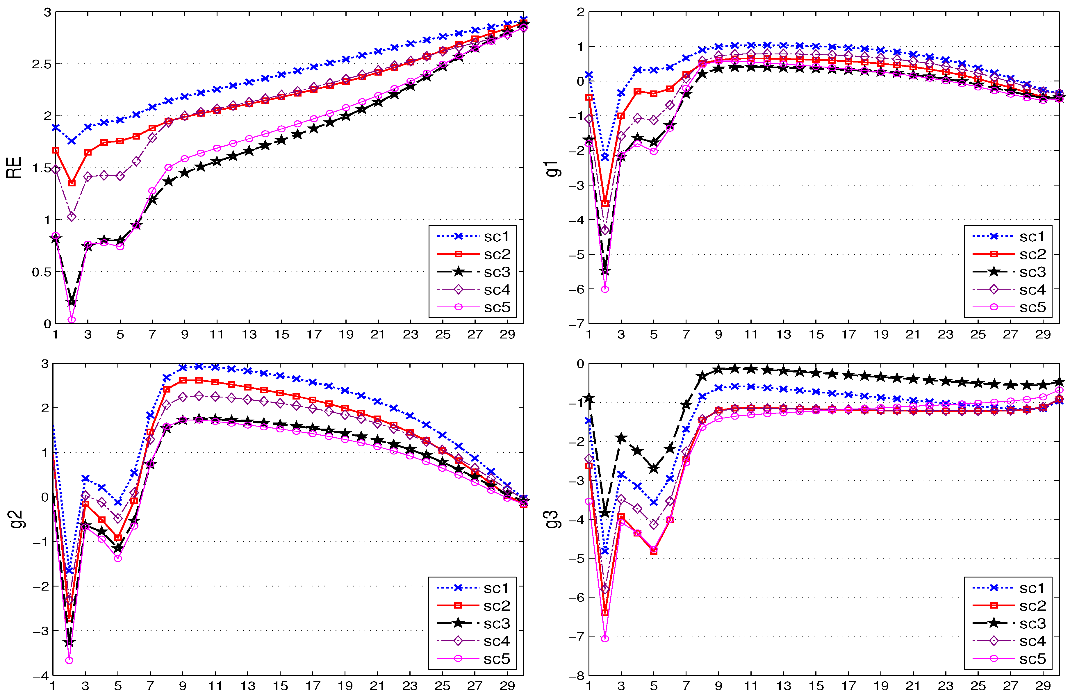
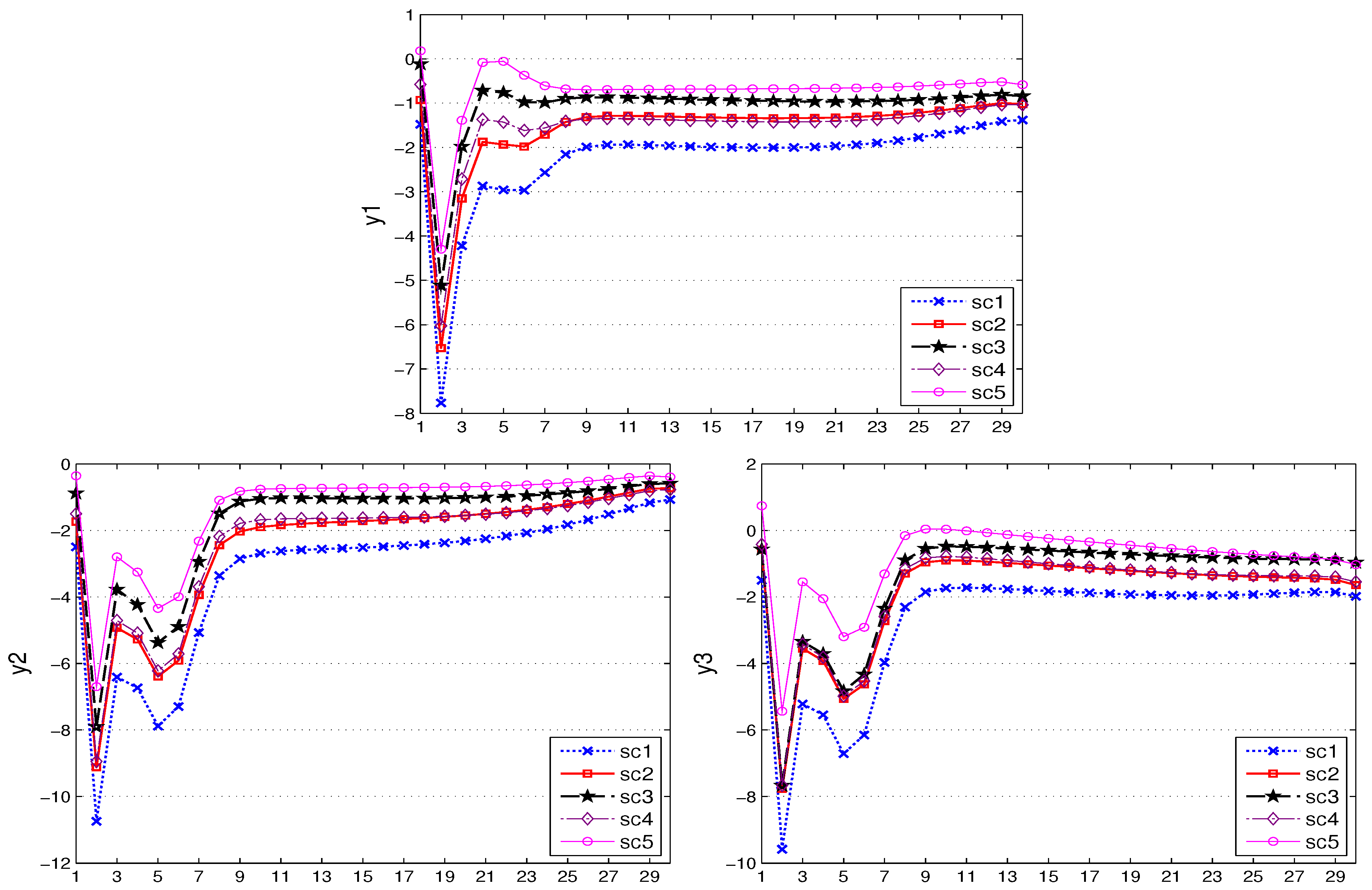
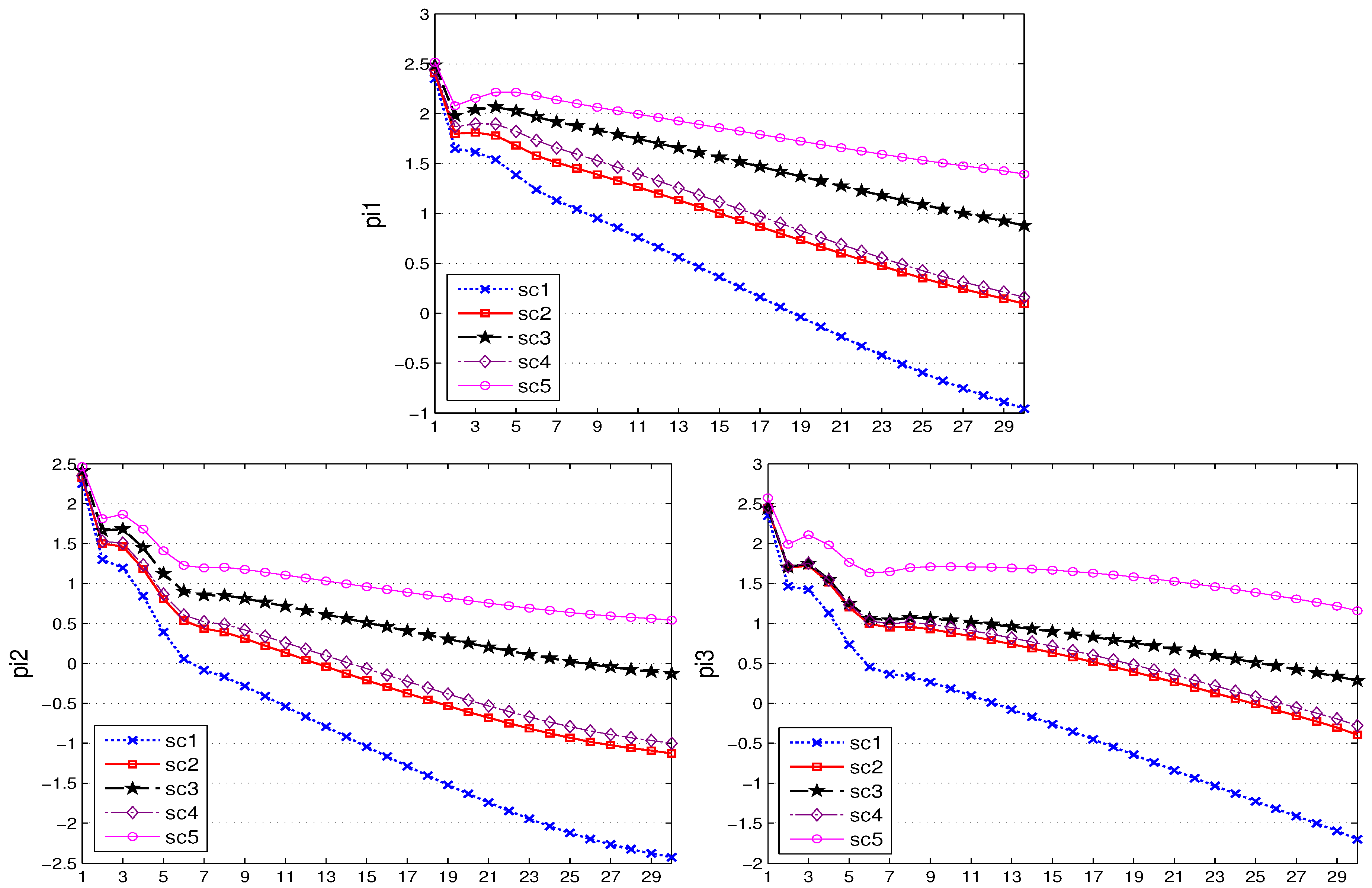
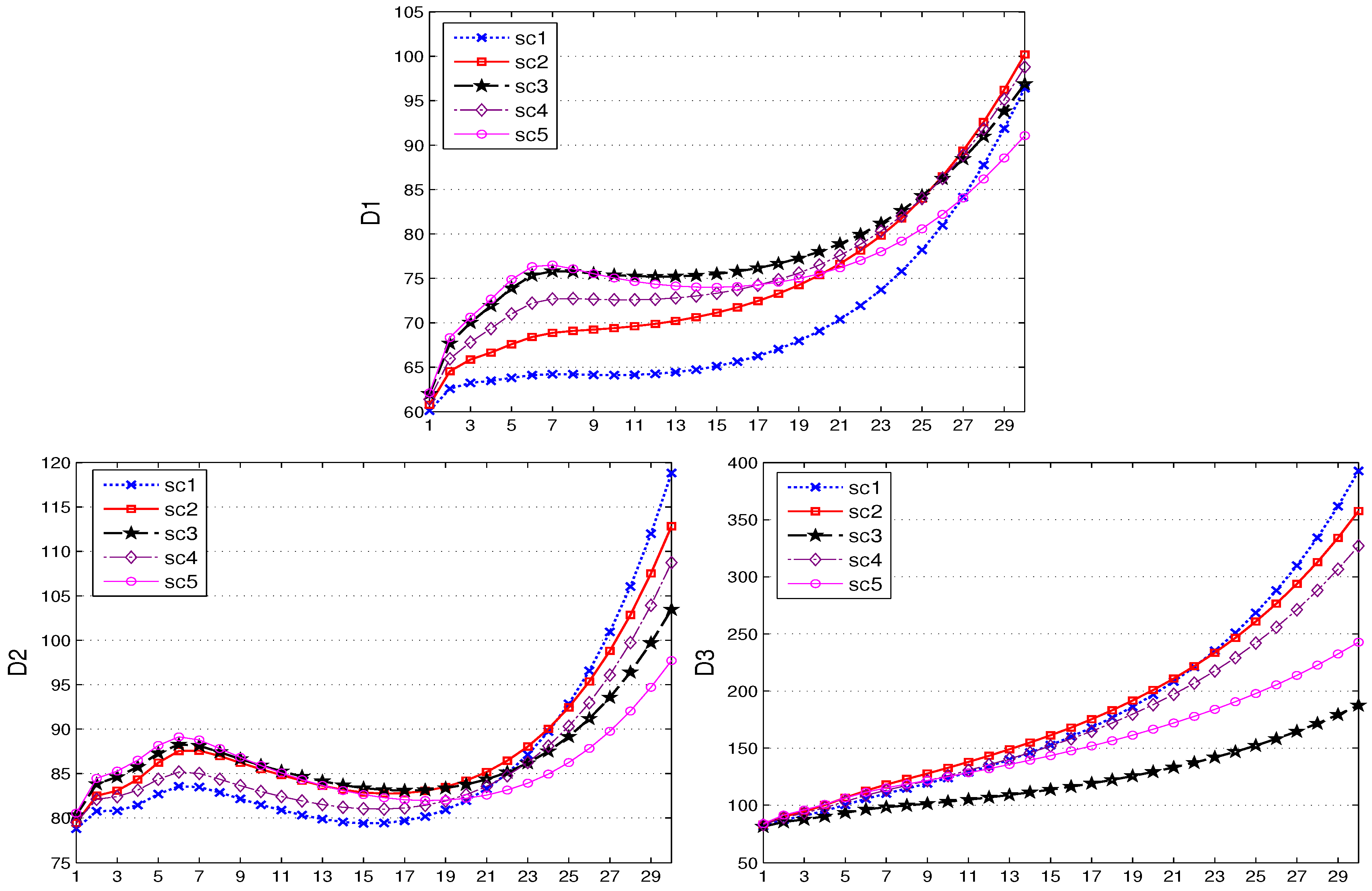
Figure 1 shows the results of the control variables in this experiment, while Figure 2, Figure 3 and Figure 4 show the results for the state variables. A first look at the graphs shows that the qualitative behavior of all policy makers is the same in each scenario: fiscal and monetary policies act in a countercyclical way, producing budget deficits and a low prime rate during the crisis, but returning to budget surpluses or at least smaller budget deficits and to the desired (long-run) prime rate after the shock is over, with fiscal policy switching back quickly and monetary policy reacting in a gradual way. The reaction to the first (global) shock is stronger than to the second (asymmetric) shock. The results for the target variables are also similar across scenarios: output remains mostly under its natural level (the zero line); rates of inflation decrease continuously (even into deflation in some scenarios); and public debt increases over the entire time horizon, especially in the thriftless country, where it reaches unsustainable levels in some scenarios.

The last column of

Table 7. Objective function values.

sc	CB	C1	C2	C3	CB + C1 + C2 + C3
sc1	183.42	113.20	319.46	233.02	849.10
sc2	140.21	81.93	216.86	184.28	623.28
sc3	228.26	77.98	140.55	94.88	541.67
sc4	150.34	85.26	192.03	161.43	589.06
sc5	203.03	66.96	102.64	120.17	492.81

presents the overall losses of all decision makers and can be interpreted in a normative way. Accordingly, the fully cooperative (Pareto-optimal) solution of Scenario 5 (the fiscal and monetary union) turns out to deliver the lowest losses, while the purely noncooperative Scenario 1 (everyone for themselves) results in the highest losses. The three coalition scenarios fare in between, with Scenario 3 coming closest to (but still differing from) the cooperative outcome and Scenario 2 coming closest to the fully-noncooperative solution. This can be interpreted to mean that, from the point of view of the policy makers involved, the best way to deal with the assumed demand shocks would be a full fiscal and monetary union, with the “throne” of the central bank shared by the bank itself and all the governments in the union. The worst solution is a policy war of everybody against everybody else. If the “throne” of the central bank has to be shared with some government(s) only, it would be better if the core and the thrifty periphery joined, but worse if only the core joined. If we compare this (admittedly extremely simplified) model of a monetary union with the Euro Area and its conflicts over macroeconomic outcomes, we may regard this result as a contribution towards explaining the position of, say, Italy (a “thrifty periphery” country with high debt, but which did not increase its debt much during the crisis) vis-à-vis Germany (the center of the core) on the one hand and Greece on the other. It also makes clear that the resistance against a leadership role for Germany in the Euro Area is not only due to historical and political reasons, but has a macroeconomic rationale behind it, as well.

Looking at the time paths of the target variables shows that the different scenarios imply some differences of outcomes that need to be explained. For the output, the situation is clear: under full cooperation, the output comes closest to its natural level, while under full non-cooperation, it remains lowest over the entire time horizon. Equally, the inflation rate is highest under cooperation and lowest (tending towards deflation) in the noncooperative equilibrium. For public debt, the effects are more complicated: the core and the thrifty periphery enjoy the lowest increase in the debt-to-GDP ratio over a rather long period, with an increase happening only during the last few years, while for the thriftless periphery, a strategy of free riding on the thrifty bloc’s coalition with the central bank allows it the smallest increase in its government debt. On the other hand, a coalition of the thriftless periphery with the central bank results in the strongest increase in its public debt. Therefore, it seems as though it would be best for the thriftless periphery not to occupy the “throne” of the central bank, but to rely on the fiscally more prudent players to do the job of implementing austerity for it. From Table 7, it is also clear that this strategy by far outperforms all the other ones, including the full fiscal and monetary union cooperation. In relation to current political discussions, the pressure placed by some highly indebted periphery countries on the core to execute a more expansionary fiscal policy comes to mind when interpreting this result.

It is also of interest how the overall losses and the losses of the single players depend on the deviation of particular objective variables.

Table 8. Detailed objective function values.

	CB			C1				C2				C3
sc	${\mathit{y}}_{\mathit{E}}$	${\mathit{\pi }}_{\mathit{E}}$	${\mathit{RE}}_{\mathit{E}}$	${\mathit{y}}_1$	${\mathit{\pi }}_1$	${\mathit{D}}_1$	${\mathit{g}}_1$	${\mathit{y}}_2$	${\mathit{\pi }}_2$	${\mathit{D}}_2$	${\mathit{g}}_2$	${\mathit{y}}_3$	${\mathit{\pi }}_3$	${\mathit{D}}_3$	${\mathit{g}}_3$
sc1	83	54	47	78	14	13	8	199	42	36	42	140	25	31	37
sc2	30	35	75	43	6	25	9	124	22	37	33	76	10	29	69
sc3	18	13	197	22	1	33	22	79	10	31	20	65	6	6	18
sc4	27	30	93	38	5	28	15	116	20	30	26	72	9	24	56
sc5	4	10	190	13	0.4	27	27	51	5	26	20	28	1	14	77

provides details on this question. It shows that the central bank in all scenarios where it acts together with some other policy maker(s) has the greatest loss from using its own instrument; only in sc1 are its losses more evenly distributed among the three variables that it is assumed to care about. This concurs with the intuition that the use of an instrument is not something that causes a welfare loss to the policy maker; instead, it is a substitute for an inequality constraint, especially in the case of a central bank that in itself cannot really be regarded as a bearer of welfare or welfare losses. On the other hand, in the scenarios with less than full cooperation, the governments nearly always get the highest welfare losses from missing natural output (which always means that they get underutilization of capacities and unemployment). Notice that there is no strong trade-off between output and public debt or budget balance: governments mostly fare better under some cooperation (especially under the overall cooperation, the full monetary and fiscal union) with respect to both variables than if they act on their own or in a partial coalition. This reinforces the argument for closer cooperation in both policy fields and for strict compliance with the rules and regulations of the policy framework by all participants.

5. Sensitivity Analysis

In this section, we present a sensitivity analysis regarding the choice of the weights. The Phillips curve trade-off between inflation and output gap in macroeconomic policy making is frequently analyzed in the literature. Thus, we consider different weights for these two objective variables in order to derive the resulting behavior of the model. The weights of the targets inflation and output gap are increased (decreased) by a factor of two (0.5) as compared to the baseline weights in Table 1. In addition, we consider an experiment where the government concentrates on inflation and output targets and drops the public debt target. This results in five different experiments as summarized in

Table 9. Robustness check experiments.

Experiment	Factor	Changed Weights
‘exp1’	$\pi$− 0.5	${\tilde{\pi }}_{it}=0.25$, ${\tilde{\pi }}_{Et}=1$,
‘exp2’	$\pi$− 2	${\tilde{\pi }}_{it}=1$, ${\tilde{\pi }}_{Et}=4$
‘exp3’	y− 0.5	${\tilde{y}}_{it}=0.5$, ${\tilde{y}}_{Et}=0.25$
‘exp4’	y− 2	${\tilde{y}}_{it}=2$, ${\tilde{y}}_{Et}=1$
‘exp5’	D− 0	${\tilde{D}}_{it}=0$

.

In the following, the results of the five different experiments are presented. The detailed objective function values are given for each experiment and can be compared to the ones presented in Table 7 and Table 8.

Table 10. Detailed objective function values, robustness experiment ‘exp1’.

	CB			C1				C2				C3				∑
sc	${\mathit{y}}_{\mathit{E}}$	${\mathit{\pi }}_{\mathit{E}}$	${\mathit{RE}}_{\mathit{E}}$	${\mathit{y}}_1$	${\mathit{\pi }}_1$	${\mathit{D}}_1$	${\mathit{g}}_1$	${\mathit{y}}_2$	${\mathit{\pi }}_2$	${\mathit{D}}_2$	${\mathit{g}}_2$	${\mathit{y}}_3$	${\mathit{\pi }}_3$	${\mathit{D}}_3$	${\mathit{g}}_3$
sc1	65	55	27	94	9	15	10	234	27	36	51	166	17	38	34	878
sc2	35	23	59	52	4	20	9	141	14	39	38	86	6	35	71	632
sc3	20	9	181	25	1	30	21	89	6	29	22	71	4	7	18	534
sc4	32	20	79	44	3	31	16	131	12	32	30	85	6	24	47	592
sc5	11	3	183	15	0.3	26	26	55	3	25	21	31	1	15	73	487

,

Table 11. Detailed objective function values, robustness experiment ‘exp2’.

	CB			C1				C2				C3				∑
sc	${\mathit{y}}_{\mathit{E}}$	${\mathit{\pi }}_{\mathit{E}}$	${\mathit{RE}}_{\mathit{E}}$	${\mathit{y}}_1$	${\mathit{\pi }}_1$	${\mathit{D}}_1$	${\mathit{g}}_1$	${\mathit{y}}_2$	${\mathit{\pi }}_2$	${\mathit{D}}_2$	${\mathit{g}}_2$	${\mathit{y}}_3$	${\mathit{\pi }}_3$	${\mathit{D}}_3$	${\mathit{g}}_3$
sc1	42	108	79	60	18	12	6	160	59	36	32	112	33	24	40	821
sc2	25	44	99	34	6	31	9	105	32	36	28	64	13	24	67	616
sc3	15	15	219	17	1	37	24	68	14	34	18	57	8	5	19	553
sc4	22	38	112	30	6	25	14	98	28	29	22	58	10	24	69	588
sc5	9	4	199	12	1	28	27	47	7	28	19	25	1	14	81	501

,

Table 12. Detailed objective function values, robustness experiment ‘exp3’.

	CB			C1				C2				C3				∑
sc	${\mathit{y}}_{\mathit{E}}$	${\mathit{\pi }}_{\mathit{E}}$	${\mathit{RE}}_{\mathit{E}}$	${\mathit{y}}_1$	${\mathit{\pi }}_1$	${\mathit{D}}_1$	${\mathit{g}}_1$	${\mathit{y}}_2$	${\mathit{\pi }}_2$	${\mathit{D}}_2$	${\mathit{g}}_2$	${\mathit{y}}_3$	${\mathit{\pi }}_3$	${\mathit{D}}_3$	${\mathit{g}}_3$
sc1	35	107	49	49	18	9	7	125	52	26	42	95	35	25	15	688
sc2	22	55	71	31	9	22	5	86	31	27	31	60	17	25	36	528
sc3	14	26	172	18	3	28	12	60	17	27	17	51	11	6	8	471
sc4	20	48	85	28	8	18	8	80	28	23	27	55	14	24	38	502
sc5	9	9	167	11	1	24	16	41	9	23	16	26	3	15	57	426

,

Table 13. Detailed objective function values, robustness experiment ‘exp4’.

	CB			C1				C2				C3				∑
sc	${\mathit{y}}_{\mathit{E}}$	${\mathit{\pi }}_{\mathit{E}}$	${\mathit{RE}}_{\mathit{E}}$	${\mathit{y}}_1$	${\mathit{\pi }}_1$	${\mathit{D}}_1$	${\mathit{g}}_1$	${\mathit{y}}_2$	${\mathit{\pi }}_2$	${\mathit{D}}_2$	${\mathit{g}}_2$	${\mathit{y}}_3$	${\mathit{\pi }}_3$	${\mathit{D}}_3$	${\mathit{g}}_3$
sc1	73	53	44	107	9	22	12	282	30	58	46	172	14	40	79	1042
sc2	35	17	80	51	3	28	17	156	13	54	41	76	4	34	120	728
sc3	17	4	229	20	0.4	37	37	90	5	37	28	68	2	6	35	615
sc4	31	15	101	42	2	46	28	146	12	45	30	79	4	24	83	687
sc5	9	1	216	12	0.3	30	40	56	2	31	29	25	0.2	14	99	565

and

Table 14. Detailed objective function values, robustness experiment ‘exp5’.

	CB			C1				C2				C3				∑
sc	${\mathit{y}}_{\mathit{E}}$	${\mathit{\pi }}_{\mathit{E}}$	${\mathit{RE}}_{\mathit{E}}$	${\mathit{y}}_1$	${\mathit{\pi }}_1$	${\mathit{D}}_1$	${\mathit{g}}_1$	${\mathit{y}}_2$	${\mathit{\pi }}_2$	${\mathit{D}}_2$	${\mathit{g}}_2$	${\mathit{y}}_3$	${\mathit{\pi }}_3$	${\mathit{D}}_3$	${\mathit{g}}_3$
sc1	26	18	4	37	3	-	13	87	9	-	35	87	9	-	35	363
sc2	17	7	6	23	1	-	27	59	4	-	47	59	4	-	47	301
sc3	13	4	18	15	0.3	-	51	52	3	-	41	59	4	-	21	281
sc4	16	7	13	21	1	-	32	63	5	-	32	61	5	-	38	293
sc5	8	1	25	10	0.2	-	59	35	1	-	45	35	1	-	45	265

present the results of these alternative simulations in terms of the welfare losses. By and large, they confirm the results from Section 4: the noncooperative scenario in general fares worst, and the full-cooperation scenario is the winner; an active monetary policy can ease pressure on fiscal policy from demands for expansionary action; Player 1 (the core country) on the whole has the lowest losses; and output losses cause more headache than the inflation rate. If these outcomes can be confirmed for more elaborate models, for example by including more players (governments or countries), then strengthening the institutional architecture of the Euro Area and the incentives to cooperative behavior may be a reasonable path towards a brighter future for the European Monetary Union.

6. Conclusions and Outlook

In this paper, we presented an application of the dynamic tracking games framework to a monetary union. We used a small stylized nonlinear three-country macroeconomic model of a monetary union to analyze the interactions between fiscal (governments) and monetary (common central bank) policy makers, assuming different objective functions of these decision makers. Using the OPTGAME algorithm, we calculated solutions for several games: a noncooperative solution where each government and the central bank play against each other (a feedback Nash equilibrium solution), a fully-cooperative solution with all players following a joint course of action (a Pareto optimal solution) and three solutions where various coalitions (subsets of the players) play against coalitions of the other players in a noncooperative way. It turns out that the fully-cooperative solution yields the best results; the noncooperative solution fares worst; and the coalition games lie in between, with a broad coalition of the fiscally more responsible countries and the central bank acting against the less thrifty country coming closest to the Pareto optimum. These results have some relevance for the current policy conflicts in the Euro Area. In order to relate them more closely to these debates, the analysis would have to be augmented by a larger number of players, a more elaborate macroeconomic model (of the DSGE type, for example) and a more sophisticated calibration of the model. These are topics for further research.