Game Theory of Tumor–Stroma Interactions in Multiple Myeloma: Effect of Nonlinear Benefits

Abstract

Cancer cells and stromal cells often exchange growth factors with paracrine effects that promote cell growth: a form of cooperation that can be studied by evolutionary game theory. Previous models have assumed that interactions between cells are pairwise or that the benefit of a growth factor is a linear function of its concentration. Diffusible factors, however, affect multiple cells and generally have nonlinear effects, and these differences are known to have important consequences for evolutionary dynamics. Here, we study tumor–stroma paracrine signaling using a model with multiplayer collective interactions in which growth factors have nonlinear effects. We use multiple myeloma as an example, modelling interactions between malignant plasma cells, osteoblasts, and osteoclasts. Nonlinear benefits can lead to results not observed in linear models, including internal mixed stable equilibria and cyclical dynamics. Models with linear effects, therefore, do not lead to a meaningful characterization of the dynamics of tumor–stroma interactions. To understand the dynamics and the effect of therapies it is necessary to estimate the shape of the benefit functions experimentally and parametrize models based on these functions.

1. Introduction

1.1. From Intra-Tumor Cooperation to Tumor–Stroma Interactions

Cancer cells secrete growth factors that promote proliferation by stimulating growth, resistance against apoptosis and against the immune system, or angiogenesis. Clones producing different essential growth factors can rely on each other for survival [1], and non-producer clones can free-ride on the growth factors produced by its cooperative neighbours [2]. The production of growth factors by cancer cells therefore is an example of intra-tumor cooperation and can be studied in the framework of evolutionary game theory. Concepts from game theory have been used to describe competition between cancer cells as pairwise games [3,4] with up to four strategies [5,6,7,8,9], and more recently as multiplayer public goods games to model the interactions between different clones within a tumor in well-mixed populations [10,11], in spatially structured populations that resemble monolayers in vitro [12,13,14], and to analyse the Warburg effect [15,16,17,18]; experiments with cancer cells have been used to test the theory [2].

Cancer cells also interact with non-cancerous stromal cells by exchanging diffusible factors [19,20,21,22] and these interactions with the tumor microenvironment are a fundamental part of cancer progression. While this is often referred to as “cooperation” between cancer and stroma, the secretion of growth factors by the stroma is often triggered by the cancer cells themselves, which recruit and activate stromal cells by producing diffusible cytokines; these cytokines stimulate the stroma to release growth factors that sustain tumor growth. Stromal cells, therefore, are manipulated by the cancer cells to produce growth factors that are beneficial to the tumor. A form of proper cooperation exists among the cancer cells themselves, as the cytokines they produce are a type of public good that can be exploited by non-producer cancer cells. Such a paracrine tumor–stroma signaling system, therefore, has non-trivial strategic interactions, which can also be studied in the framework of evolutionary game theory, but have received relatively less attention so far. Tumor–stroma interactions have been analysed in the context of prostate cancer [8], multiple myeloma [5,23], and MMP–TIMP (matrix metalloproteinases and tissue inhibitors of metalloproteinases) interactions [24].

1.2. From Two-Player Games to Collective Interactions with Nonlinear Effects

One problem with early models of tumor–stroma interactions, as with early models of intra-tumor cooperation, is that they assume pairwise interactions between cells. Cells, however, compete with more than one neighbor, and multiple cells contribute to the overall amount of growth factors available to a cell. A model with collective interactions [23] has been shown to lead to different results compared to a model [5] with pairwise interactions, with implications for disease progression and treatment (in particular, this new model suggests that reducing the number of malignant plasma cells below a critical threshold can lead to their extinction and thus to restore a healthy balance between osteoclast and osteoblast).

Even this approach, however, made an unrealistic assumption: that the effect of the growth factors exchanged by the cells is a linear function of its concentration. While linear effects are more amenable to analytical study, it is known that most growth factors have a nonlinear, often sigmoid, effect on cell proliferation, and that nonlinear effects can lead to very different dynamics [25,26]. We decided, therefore, to analyse tumor–stroma interactions using a multiplayer public goods game with nonlinear benefits, sacrificing analytical tractability for the sake of realism. Our goal is to understand whether nonlinear effects lead to qualitatively different results in the dynamics and equilibria in the study of tumor–stroma interactions, in particular in multiple myeloma (a type of cancer of plasma cells [27,28]).

1.3. Multiple Myeloma as a Modelling Case Study

We use multiple myeloma as a case study, continuing a previous extension to multiplayer linear games [23] of an earlier model with pairwise interactions [5]. In multiple myeloma, interleukin-6 (IL6), which promotes tumor proliferation, is produced not only by malignant plasma cells, but also by bone marrow stromal cells and osteoblasts; the stroma, however, is induced to produce IL6 by cytokines secreted by the multiple myeloma cells themselves [29,30], including FGF-beta [31], IL-1 [32], TNF-alpha [33], TGF-1 [34], and VEGF [35]. More in general, in multiple myeloma three types of cells contribute to bone resorption and bone formation by exchanging diffusible factors: malignant plasma cells (multiple myeloma, MM), osteoclasts (OC), and osteoblasts (OB). MM cells produce cytokines that activate OC and inhibit OB, altering the normal OB–OC equilibrium of healthy cells (and inducing, among other symptoms, bone fracture typical of multiple myeloma). OC and OB also secrete growth factors that affect each other and MM cells [36,37]. Our model is consistent with assumptions used previously in a model with linear benefits [23]—which was itself an extension with collective interactions of a pairwise game [5]—with the difference that here we use nonlinear benefit functions.

2. Results

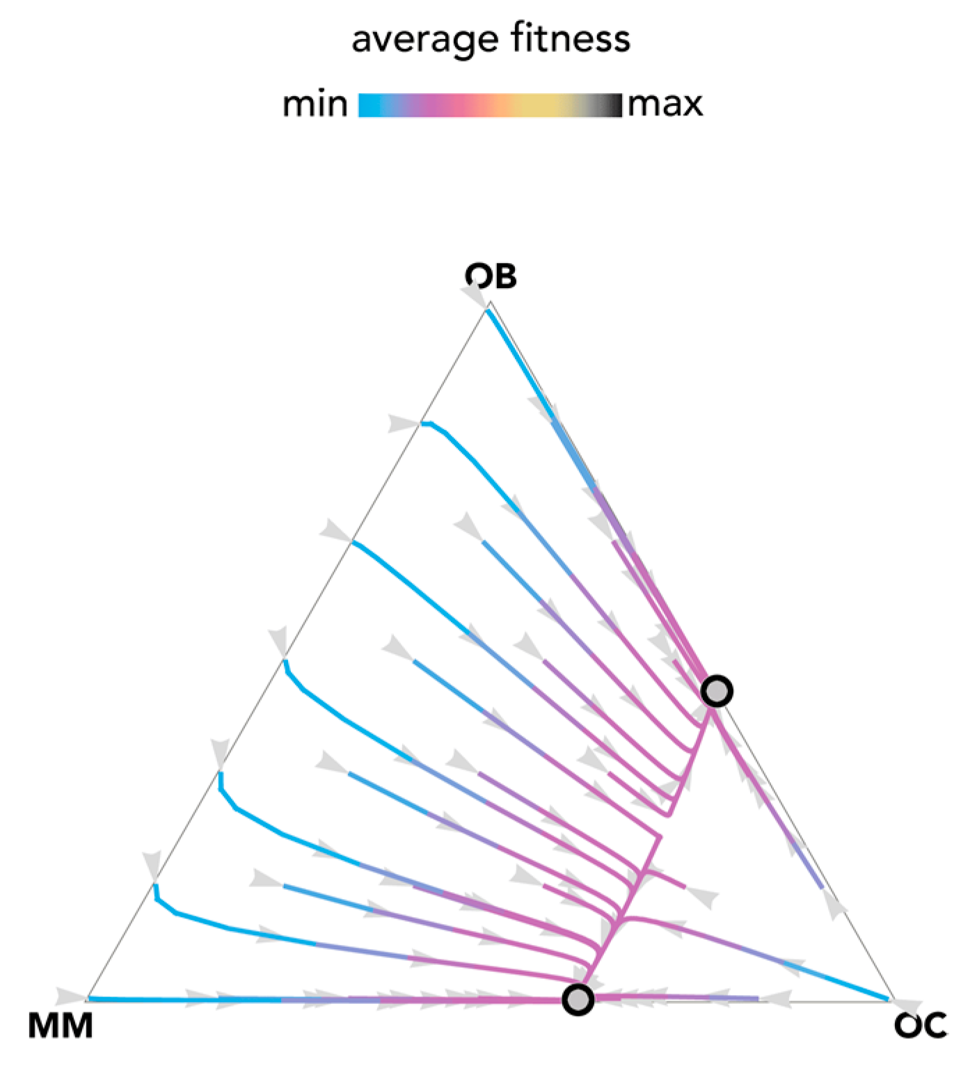
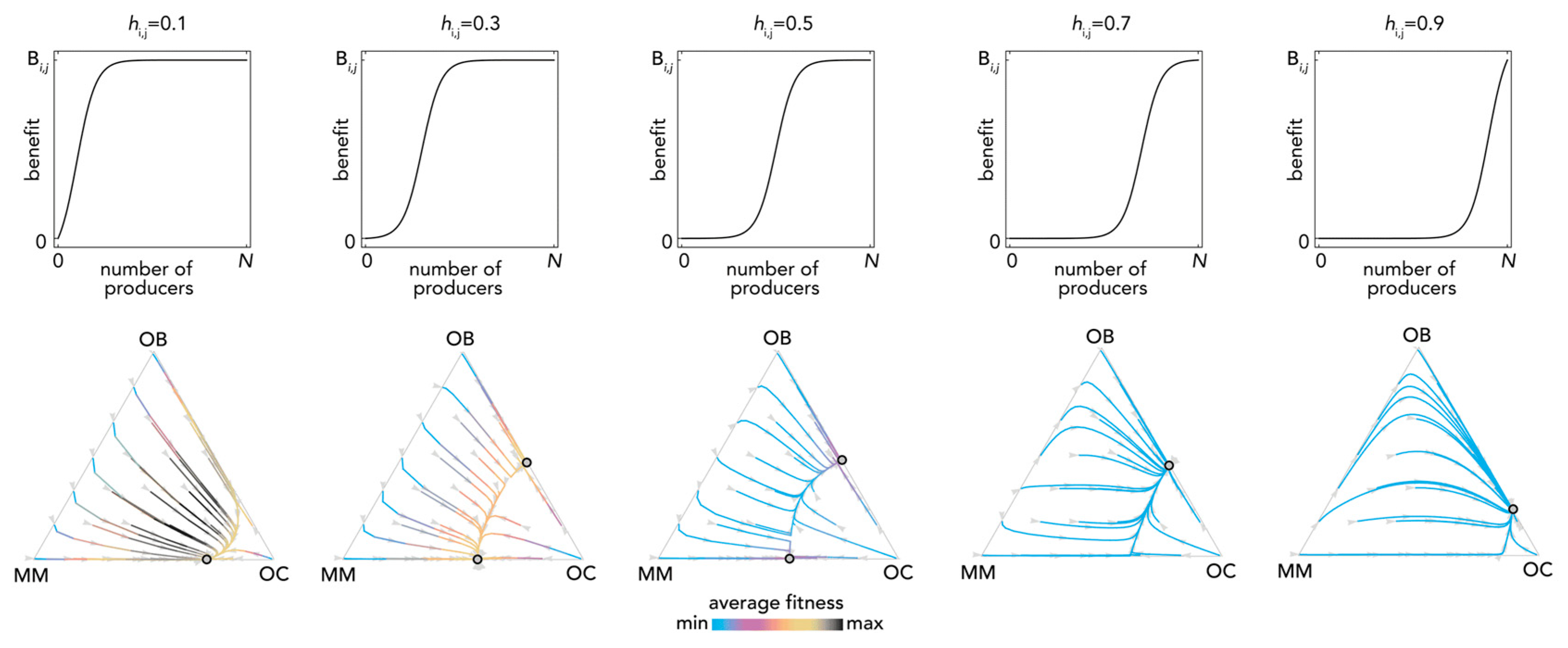
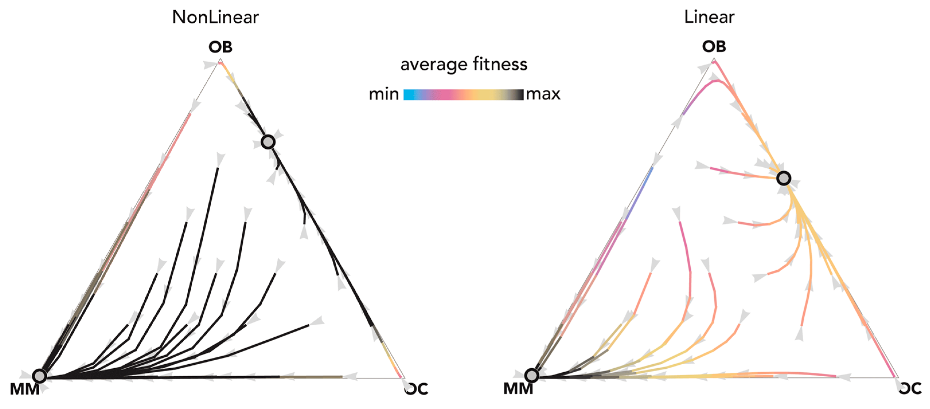
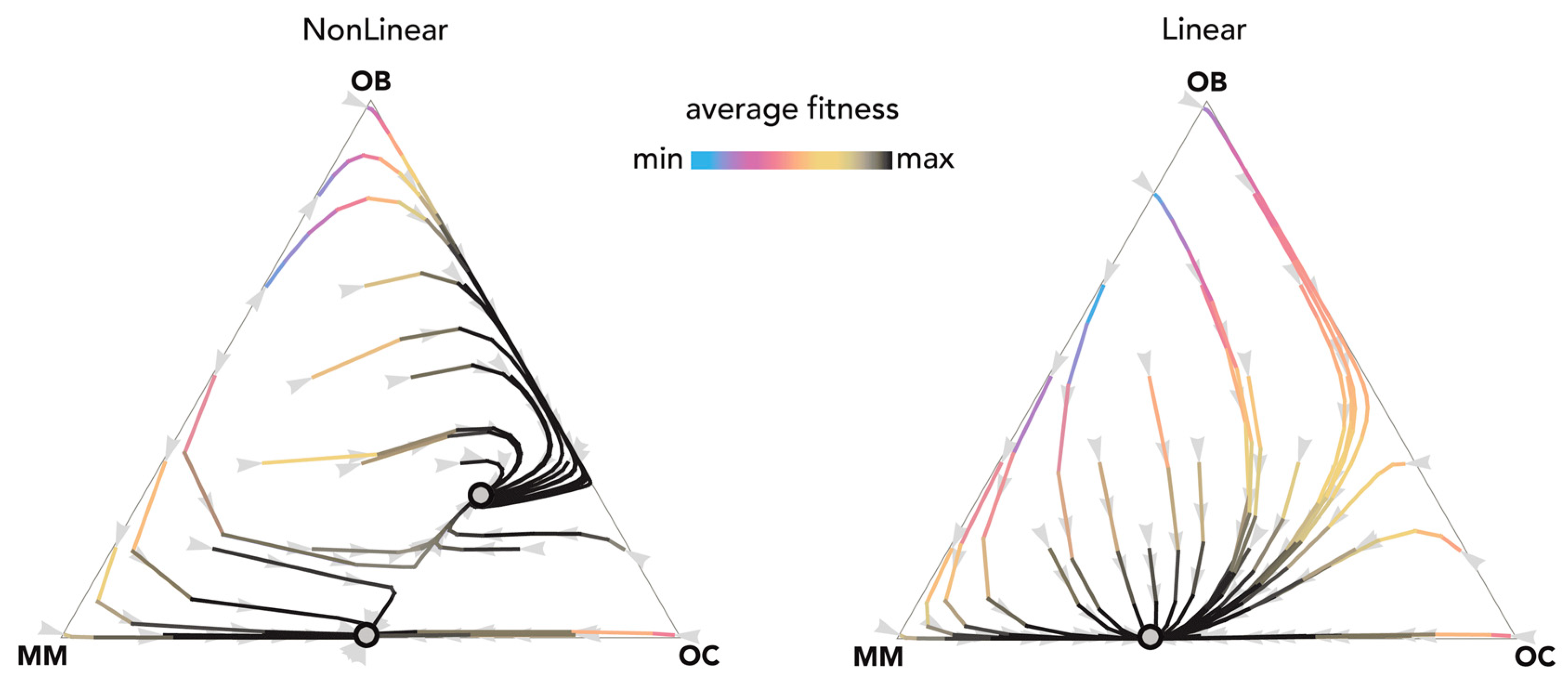
2.1. Stability (Bistability) Depends on the Shape of the Benefit Functions

The most fundamental result of previous models is described in Figure 1: OB and OC cells are at a mixed equilibrium, balancing each other until MM cells are introduced in the population: if enough MM cells are introduced, the population evolves to a stable equilibrium on the MM–OC edge, which explains the potential for bone fractures observed in multiple myeloma. This result is obtained for the special case s_i,j→0 (linear benefits) in our model, and is consistent with previous models of linear benefits [23]. Observe, however (Figure 2), that if benefits are nonlinear this is not necessarily the case: the OB–OC equilibrium can persist irrespective of the number of MM cells introduced in the population or disappear entirely, depending on the shape of the benefit functions (in Figure 2 the position of the inflection point). While a model with linear benefits predicts a bistable system, nonlinear benefits can have both or only one of the two stable equilibria observed in linear models. Further examples are shown in Figure 3 and Figure 4, where additional mixed equilibria, not observed with linear benefits, arise with nonlinear benefits; in other cases, instead, the dynamics are similar (Figure 5). Unfortunately, given the huge number of combinations of parameters in the nonlinear model, any useful generalization is impossible. To understand and predict the dynamics of the system we need to know the shape of the benefit functions.

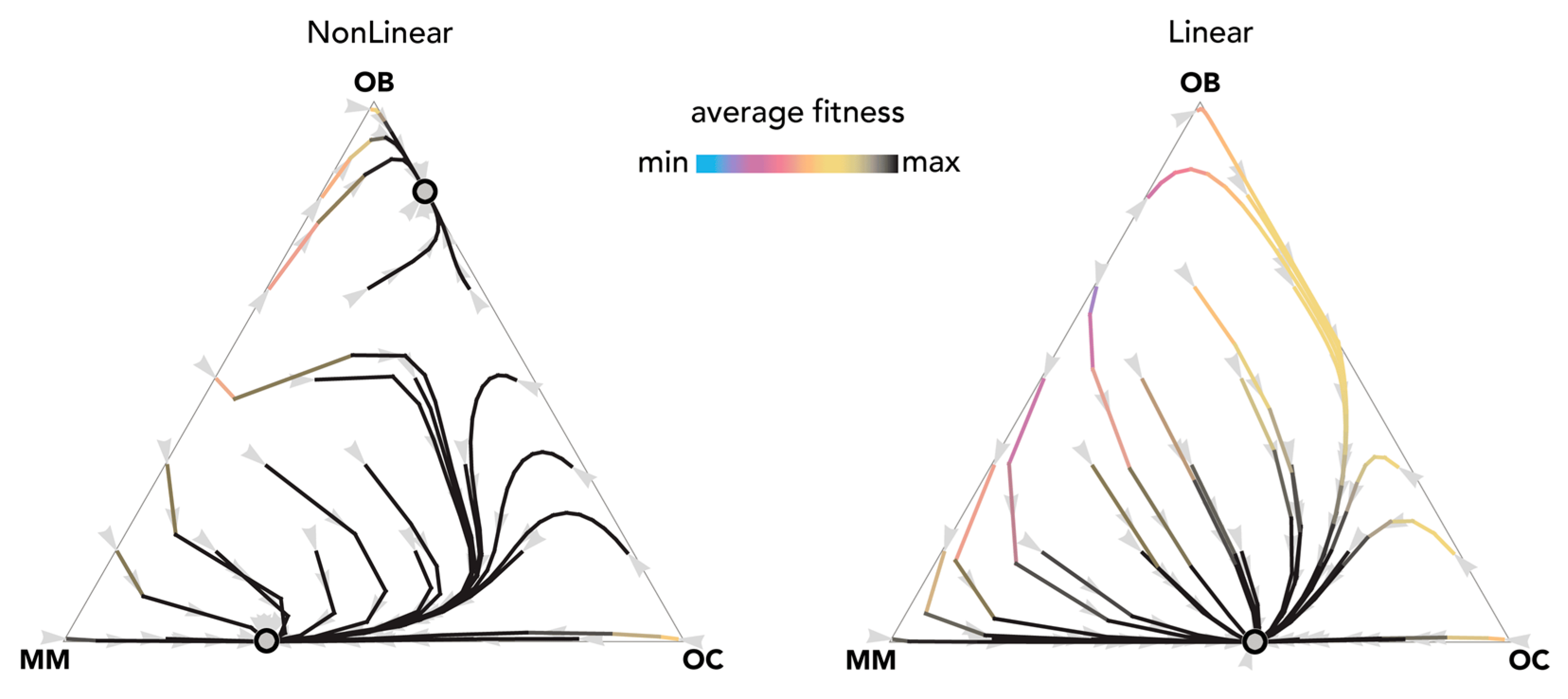
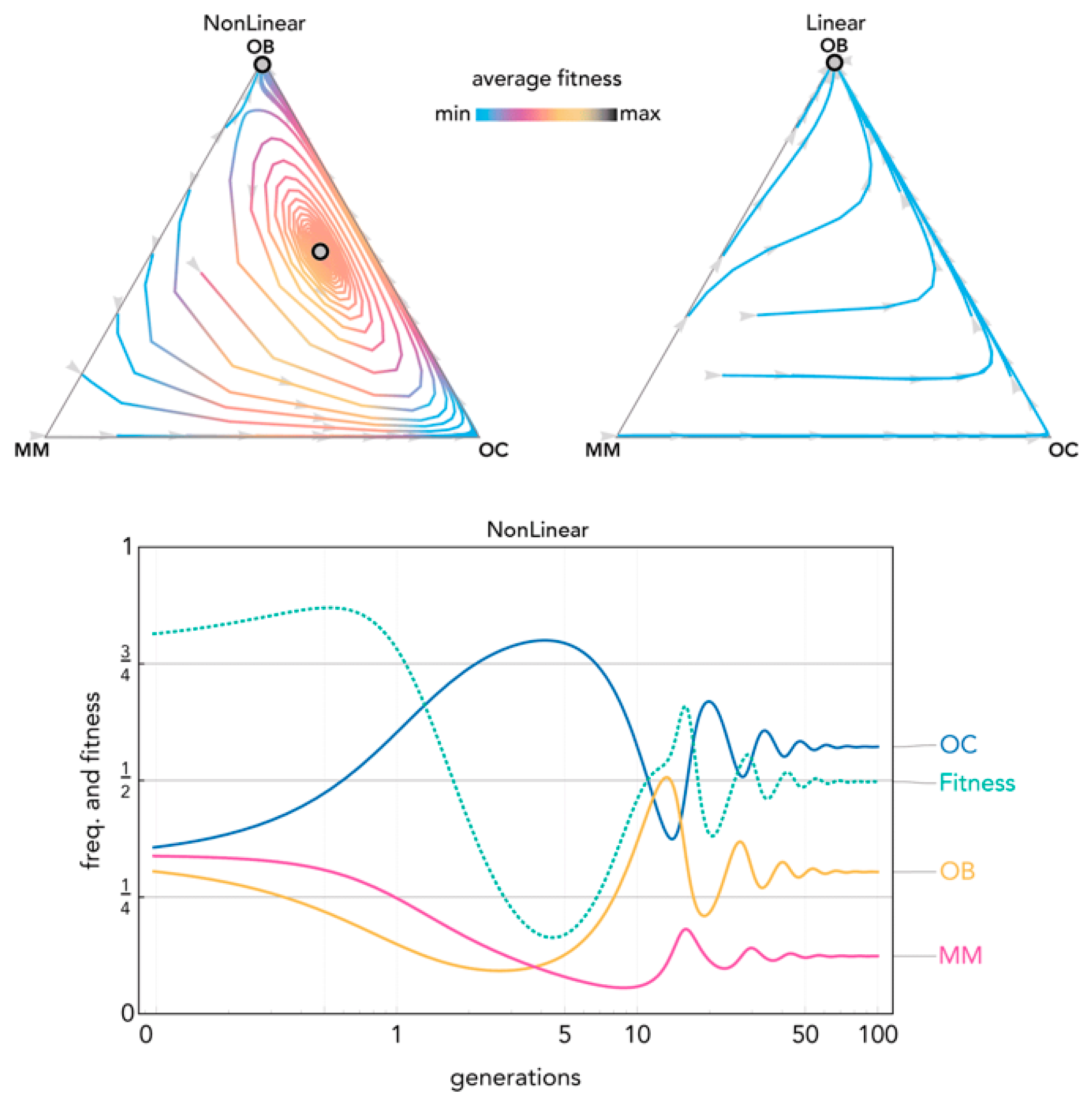
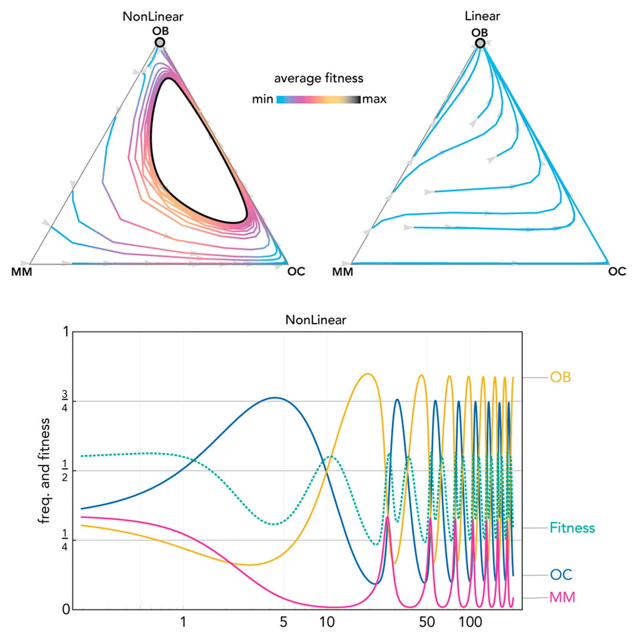
2.2. Nonlinear Benefits Can Lead to the Coexistence of Three Types and Cyclical Dynamics

Nonlinear benefits introduce a new type of equilibrium, never observed in linear models, in which all three types coexist (Figure 6). Coexistence of the three types can also be reached with cyclical oscillations that converge to a stable equilibrium (Figure 7) and even persist as a limit cycle (Figure 8): two types of dynamics that are never observed in linear models (and, more in general, in public goods games with constant group size).

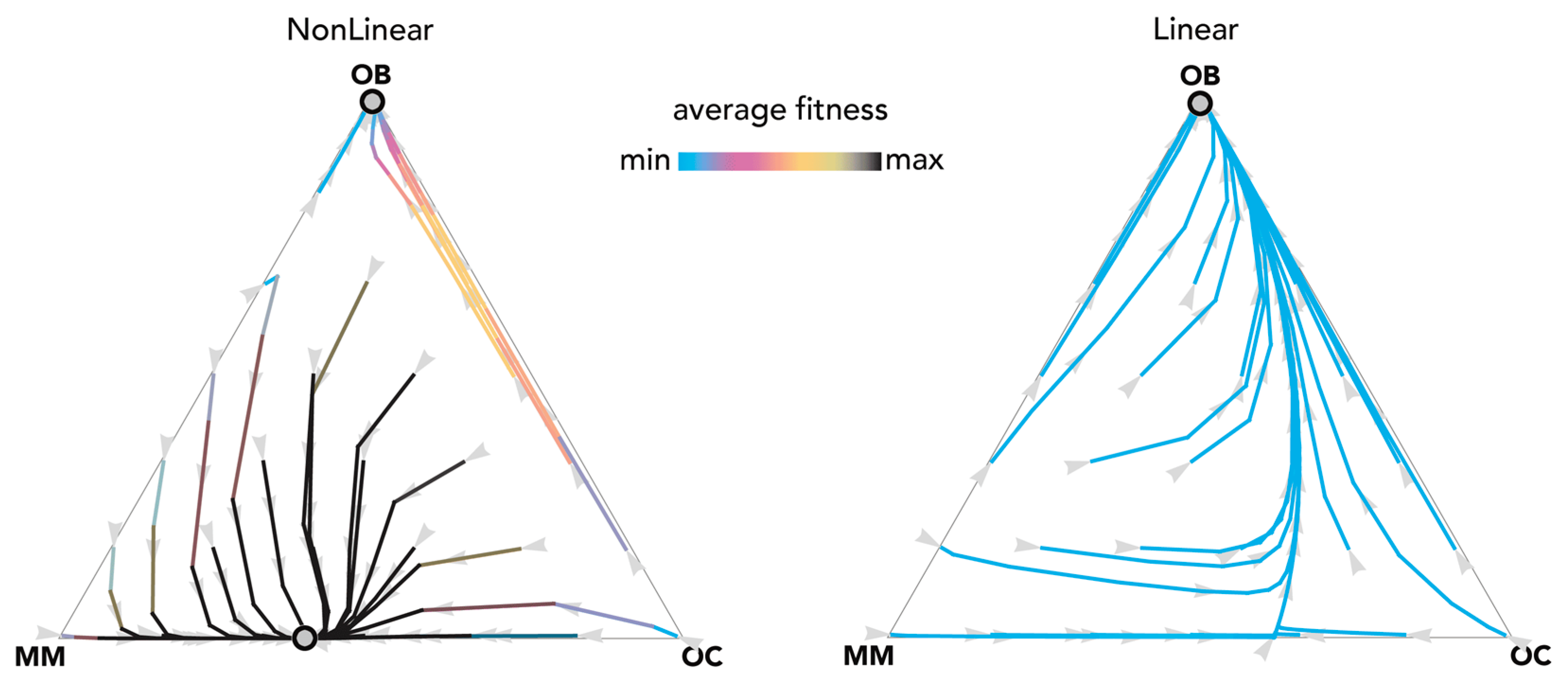
2.3. Therapies That Target Growth Factors May Be More Effective Than Chemotherapy

Perturbations of the equilibria can reveal the effect of therapies against multiple myeloma and help understand the evolution of resistance to therapies. Figure 9 shows an example. At the OB–OC equilibrium, a mutant MM clone invades the population and leads to a MM–OC equilibrium: the typical fundamental result of current models (see Figure 1). A therapy that reduces the fraction of MM cells (such as chemotherapy that targets MM cells) immediately reduces the average fitness of the population; MM cells, however, eventually increase in frequency again and the population moves back to the previous MM–OC equilibrium. A therapy that increases the position of the inflection point (see Figure 2), for instance targeting the growth factors produced by the stroma and by the tumor (the inflection point increases when some of the growth factors are removed or made unavailable by the therapy because additional growth factors must be secreted—hence more producer cells are necessary—in order to achieve the same pre-therapy benefit level), instead, could lead to a spontaneous extinction of the MM types and a reduction of fitness; that is, a reduction in the speed of tumor growth. Understanding the effects of the two approaches quantitatively requires an estimation of the shape of the benefit functions.

3. Discussion

In summary, in addition to the pure equilibria and the two-type mixed equilibria observed in linear models [23], two additional results arise when benefits are nonlinear benefits: a mixed stable equilibrium with three types; and cyclical dynamics of the three types. This reconciles evolutionary game theory models with observations in real tumors (where the three types of cells can clearly coexist — something that previous linear models could not account for).

Our results, however, also show that it is impossible to generalize the results and predict the dynamics of the system without knowing exactly the shape of the benefit functions; small changes can lead to very different dynamics. In order to understand the dynamics and to be able to predict the effect of therapies, the shape of these benefit functions must be estimated from experimental data.

Even though, in the absence of measures of the shape of the benefit functions, we cannot yet provide an exact description of the dynamics and suggest how to calibrate therapies, our results suggest that a therapy will be more effective if, in addition, or even in alternative, to reducing the amount of MM cells, it increases the value of the inflection point of the benefit functions, which could be achieved, for example, using monoclonal antibodies against the growth factors produced by the tumor and the stroma (still an experimental approach [38,39]). Monoclonal antibodies increase the value of the inflection point because they make some of the secreted growth factors unavailable to the tumor; hence, further growth factors must be produced—hence more producer cells are necessary—in order to achieve the same pre-therapy benefit level. Reducing the amount of MM cells, instead, does not affect the shape of the benefit function. In other words, therapies that change the parameters of the game may be more effective, and lead to a stable outcome, than therapies that change the frequency of the players.

More in general, besides multiple myeloma, our results show that models with linear benefits (not to mention models with pairwise interactions) do not provide a reliable characterization of the dynamics of tumor–stroma interactions, and that unexpected types of dynamics, such as cyclical dynamics, can arise due to nonlinearities.

4. Materials and Methods

Let us call x_OC, x_OB, and x_MM the frequencies of three types of cells, respectively OC (osteoclasts), OB (osteoblasts), and MM (malignant plasma cells), in the population (x_OC + x_OB + x_MM = 1). N is the number of cells within the diffusion range of the growth factors (hence, equal to group size), which we assume is the same for all types and all growth factors. Fitness is calculated by considering the payoffs obtained in the randomly formed groups weighted by the probability that such groups occur. In a well-mixed population, the probability that a group contains n_OC, n_OB, and N − n_OC − n_OB individuals (excluding the focal cell itself) of type OC, OB, and MM, respectively, is given by

$$\left(\begin{array}{c}N-1\\ n_{OC},n_{OB}\end{array}\right)x_{OC}{}^{n_{OC}}·x_{OB}{}^{n_{OB}}·x_{MM}{}^{N-n_{OB}-n_{OC}-1}.$$

(1)

The payoffs for OC, OB, and MM are, respectively:

V_OC = b_OC,OC(n_OC + 1) + b_OB,OC(n_OB) + b_MM,OC(N − 1 − n_OC − n_OB) − c_OC

(2)

V_OB = b_OC,OB(n_OC) + b_OB,OB(n_OB + 1) + b_MM,OB(N − 1 − n_OC − n_OB) − c_OB

(3)

V_MM = b_OC,MM(n_OC) + b_OB,MM(n_OB) + b_MM,MM(N − n_OC − n_OB) − c_MM

(4)

where c_i is the cost of producing growth factors by type i and b_i,j is a function that indicates the effect on type j of the growth factors produced by type i. Note that each player’s strategy has also an effect on itself. The fitness of type i is given by

$$W_i={\displaystyle \sum }_{n_{OC}=1}^{N-1}{\displaystyle \sum }_{n_{OB}=0}^{N-1-n_{OC}}\left(\begin{array}{c}N-1\\ n_{OC},n_{OB}\end{array}\right)x_{OC}{}^{n_{OC}}·x_{OB}{}^{n_{OB}}·x_{MM}{}^{N-n_{OB}-n_{OC}-1}·V_i.$$

(5)

The frequencies change based on the replicator dynamics:

x_OC′ = x_OC(W_OC − W *)

(6)

x_OB′ = x_OB(W_OB − W *)

(7)

x_MM′ = x_MM(W_MM − W *)

(8)

where W * = x_OCW_OC + x_OBW_OB + x_MMW_MM. To introduce nonlinearities, we assume a benefit function defined by

$$b_{i,j}\left(n_i\right)=\frac{\left[l_{i,j}\left(n_i\right)-l_{i,j}\left(0\right)\right]}{\left[l_{i,j}\left(N\right)-l_{i,j}\left(0\right)\right]}$$

(9)

the normalized version of the logistic function

$$l_{i,j}\left(n_i\right)=\frac{B_{i,j}}{1+e^{s_{i,j}\left(h_{i,j}-n_i/N\right)}}$$

(10)

where n_i is the number of cells of type i; the parameters define the effect of the growth factors produced by type i on type j: B_i,j defines the maximum benefit; h_i,j defines the position of the inflection point: h_i,j→1 gives increasing returns and h_i,j→0 diminishing returns; s_i,j defines the steepness of the function at the inflection point (s_i,j→∞ models a threshold public goods game; s_i,j→0 models a linear benefit (Figure 10); and the normalization in (9) in prevents the logistic function (10) from becoming constant for s_i,j→0).

References

1. Axelrod, R.; Axelrod, D.E.; Pienta, K.J. Evolution of cooperation among tumor cells. Proc. Natl. Acad. Sci. USA 2006, 103, 13474–13479. [Google Scholar] [CrossRef] [PubMed]
2. Archetti, M.; Ferraro, D.A.; Christofori, G. Heterogeneity for IGF-II production maintained by public goods dynamics in neuroendocrine pancreatic cancer. Proc. Natl. Acad. Sci. USA 2015, 112, 1833–1838. [Google Scholar] [CrossRef] [PubMed] [Green Version]
3. Tomlinson, I.P. Game-theory models of interactions between tumour cells. Eur. J. Cancer 1997, 33, 1495–1500. [Google Scholar] [CrossRef]
4. Tomlinson, I.P.; Bodmer, W.F. Modelling consequences of interactions between tumour cells. Br. J. Cancer 1997, 75, 157–160. [Google Scholar] [CrossRef] [PubMed]
5. Dingli, D.; Chalub, F.; Santos, F.; Van Segbroeck, A.; Pacheco, J. Cancer phenotype as the outcome of an evolutionary game between normal and malignant cells. Br. J. Cancer 2009, 101, 1130–1136. [Google Scholar] [CrossRef] [PubMed]
6. Basanta, D.; Simon, M.; Hatzikirou, H.; Deutsch, A. Evolutionary game theory elucidates the role of glycolysis in glioma progression and invasion. Cell Prolif. 2008, 41, 980–987. [Google Scholar] [CrossRef] [PubMed]
7. Basanta, D.; Deutsch, A. A game theoretical perspective on the somatic evolution of cancer. In Selected Topics on Cancer Modelling: Genesis Evolution Immune Competition Therapy; Bellomo, N., Chaplain, M., De Angelis, E., Eds.; Birkhauser Boston: Cambridge, MA, USA, 2008. [Google Scholar]
8. Basanta, D.; Scott, J.G.; Fishman, M.N.; Ayala, G.; Hayward, S.W.; Anderson, A.R. Investigating prostate cancer tumour-stroma interactions: Clinical and biological insights from an evolutionary game. Br. J. Cancer 2012, 106, 174–181. [Google Scholar] [CrossRef] [PubMed] [Green Version]
9. Gerstung, M.; Nakhoul, H.; Beerenwinkel, N. Evolutionary games with affine fitness functions: Applications to cancer. Dyn. Games Appl. 2011, 1, 370–385. [Google Scholar] [CrossRef]
10. Archetti, M. Evolutionary game theory of growth factor production: Implications for tumor heterogeneity and resistance to therapies. Br. J. Cancer 2013, 109, 1056–1062. [Google Scholar] [CrossRef] [PubMed] [Green Version]
11. Archetti, M. Evolutionarily stable anti-cancer therapies by autologous cell defection. Evol. Med. Public Heatlh 2013, 1, 161–172. [Google Scholar] [CrossRef] [PubMed]
12. Archetti, M. Dynamics of growth factor production in monolayers of cancer cells. Evol. Appl. 2013, 6, 1146–1159. [Google Scholar] [CrossRef] [PubMed] [Green Version]
13. Archetti, M. Stable heterogeneity for the production of diffusible factors in cell populations. PLoS ONE 2014, 9, e108526. [Google Scholar] [CrossRef] [PubMed] [Green Version]
14. Archetti, M. Cooperation among cancer cells as public goods games on Voronoi networks. J. Theor. Biol. 2016, 396, 191–203. [Google Scholar] [CrossRef] [PubMed] [Green Version]
15. Basanta, D.; Hatzikirou, H.; Deutsch, A. Studying the emergence of invasiveness in tumours using game theory. Eur. Phys. J. 2008, 63, 393–397. [Google Scholar] [CrossRef]
16. Basanta, D.; Scott, J.G.; Rockne, R.; Swanson, K.R.; Anderson, A.R. The role of IDH1 mutated tumour cells in secondary glioblastomas: An evolutionary game theoretical view. Phys. Biol. 2011, 8, 15016. [Google Scholar] [CrossRef] [PubMed]
17. Archetti, M. Evolutionary dynamics of the Warburg effect: Glycolysis as a collective action problem among cancer cells. J. Theor. Biol. 2014, 341, 1–8. [Google Scholar] [CrossRef] [PubMed] [Green Version]
18. Archetti, M. Heterogeneity and proliferation of invasive cancer subclones in game theory models of the Warburg effect. Cell Prolif. 2015, 48, 259–269. [Google Scholar] [CrossRef] [PubMed] [Green Version]
19. Li, H.; Fan, X.; Houghton, J. Tumor microenvironment: The role of the tumor stroma in cancer. J. Cell. Biochem. 2007, 101, 805–815. [Google Scholar] [CrossRef] [PubMed]
20. Pietras, K.; Ostman, A. Hallmarks of cancer: Interactions with the tumor stroma. Exp. Cell Res. 2010, 316, 1324–1331. [Google Scholar] [CrossRef] [PubMed]
21. Cirri, P.; Chiarugi, P. Cancer associated fibroblasts: The dark side of the coin. Am. J. Cancer Res. 2011, 1, 482–497. [Google Scholar] [PubMed]
22. Hanahan, D.; Coussens, L.M. Accessories to the crime: Functions of cells recruited to the tumor microenvironment. Cancer Cell 2012, 21, 309–322. [Google Scholar] [CrossRef] [PubMed]
23. Sartakhti, J.S.; Manshaei, M.H.; Bateni, S.; Archetti, M. Evolutionary Dynamics of Tumor-Stroma Interactions in Multiple Myeloma. PLoS ONE 2016, 11, e0168856. [Google Scholar] [CrossRef] [PubMed]
24. Sartakhti, J.S.; Manshaei, M.H.; Sadeghi, M. MMP–TIMP interactions in cancer invasion: An evolutionary game- theoretical framework. J. Theor. Biol. 2017, 412, 17–26. [Google Scholar] [CrossRef] [PubMed]
25. Archetti, M.; Scheuring, I. Review: Evolution of cooperation in one-shot social dilemmas without assortment. J. Theor. Biol. 2012, 299, 9–20. [Google Scholar] [CrossRef] [PubMed]
26. Archetti, M. How to analyze models of nonlinear public goods. Games 2018, 9, 17. [Google Scholar] [CrossRef]
27. Roodman, G. Pathogenesis of myeloma bone disease. Leukemia 2009, 23, 435–441. [Google Scholar] [CrossRef] [PubMed]
28. Yaccoby, S. Advances in the understanding of myeloma bone disease and tumour growth. Br. J. Haematol. 2010, 149, 311–321. [Google Scholar] [CrossRef] [PubMed]
29. Manier, S.; Sacco, A.; Leleu, X.; Ghobrial, I.M.; Roccaro, A.M. Bone marrow microenvironment in multiple myeloma progression. J. Biomed. Biotechnol. 2012, 2012, 157496. [Google Scholar] [CrossRef] [PubMed]
30. Shalaby, M.R.; Waage, A.; Espevik, T. Cytokine regulation of interleukin-6 production by human endothelial cells. Cell. Immunol. 1989, 121, 372–382. [Google Scholar] [CrossRef]
31. Bisping, G.; Leo, R.; Wenning, D.; Dankbar, B.; Padró, T.; Kropff, M.; Scheffold, C.; Kröger, M.; Mesters, R.M.; Berdel, W.E.; et al. Paracrine interactions of basic fibroblast growth factor and interleukin-6 in multiple myeloma. Blood 2003, 101, 2775–2783. [Google Scholar] [CrossRef] [PubMed]
32. Dinarello, C.A. Interleukin-1 in the pathogenesis and treatment of inflammatory diseases. Blood 2011, 117, 3720–3732. [Google Scholar] [CrossRef] [PubMed]
33. Carter, A.; Merchav, S.; Silvian-Draxler, I.; Tatarsky, I. The role of interleukin-1 and tumor necrosis factor-alpha in human multiple myeloma. Br. J. Haematol. 1990, 74, 424–431. [Google Scholar] [CrossRef] [PubMed]
34. Urashima, M.; Ogata, A.; Chauhan, D.; Hatziyanni, M.; Vidriales, M.B.; Dedera, D.A.; Schlossman, R.L.; Anderson, K.C. Transforming growth factor-beta1: Differential effects on multiple myeloma versus normal B cells. Blood 1996, 87, 1928–1938. [Google Scholar] [PubMed]
35. Dankbar, B.; Padró, T.; Leo, R.; Feldmann, B.; Kropff, M.; Mesters, R.M.; Serve, H.; Berdel, W.E.; Kienast, J. Vascular endothelial growth factor and interleukin-6 in paracrine tumor-stromal cell interactions in multiple myeloma. Blood 2000, 95, 2630–2636. [Google Scholar] [PubMed]
36. Ehrlich, L.A.; Chung, H.Y.; Ghobrial, I.; Choi, S.J.; Morandi, F.; Colla, S.; Rizzoli, V.; Roodman, G.D.; Giuliani, N. IL-3 is a potential inhibitor of osteoblast differentiation in multiple myeloma. Blood 2005, 106, 1407–1414. [Google Scholar] [CrossRef] [PubMed]
37. Lee, J.W.; Chung, H.Y.; Ehrlich, L.A.; Jelinek, D.F.; Callander, N.S.; Roodman, G.D.; Choi, S.J. IL-3 expression by myeloma cells increases both osteoclast formation and growth of myeloma cells. Blood 2004, 103, 2308–2315. [Google Scholar] [CrossRef] [PubMed]
38. Trikha, M.; Corringham, R.; Klein, B.; Rossi, J.F. Targeted anti-interleukin-6 monoclonal antibody therapy for cancer: A review of the rationale and clinical evidence. Clin. Cancer Res. 2003, 9, 4653–4665. [Google Scholar] [PubMed]
39. Lonial, S.; Durie, B.; Palumbo, A.; San-Miguel, J. Monoclonal antibodies in the treatment of multiple myeloma: Current status and future perspectives. Leukemia 2016, 30, 526–535. [Google Scholar] [CrossRef] [PubMed]
Figure 1. Bistability with linear benefits. The distance from each vertex is inversely proportional to the frequency of each type. Arrows show the direction of the dynamics; colors show the average fitness of the population. N = 10; cOC = 0.1; cOB = 0.2; cMM = 0.3; BOC,OC = 0; BOC,OB = 1; BOC,MM = 1.1; BOB,OC = 1; BOB,OB = 0; BOB,MM = 0; BMM,OC = 1.1; BMM,OB = −0.3; BMM,MM = 0; si,j→0.
Games 09 00032 g001
Figure 2. Bistability with nonlinear benefits. The top panels show the benefit function for different values of hi,j. In the bottom panels, the distance from each vertex is inversely proportional to the frequency of each type; arrows show the direction of the dynamics; colors show the average fitness of the population. N = 10; cOC = 0.1; cOB = 0.2; cMM = 0.3; BOC,OC = 0; BOC,OB = 1; BOC,MM = 1.1; BOB,OC = 1; BOB,OB = 0; BOB,MM = 0; BMM,OC = 1.1; BMM,OB = −0.3; BMM,MM = 0; si,j = 20.
Games 09 00032 g002
Figure 3. Nonlinear benefits can lead to an additional mixed equilibrium on the OB–OC edge. The distance from each vertex is inversely proportional to the frequency of each type. Arrows show the direction of the dynamics; colors show the average fitness of the population. N = 25; ci = 0.1; BOC,OC = 0.6; BOC,OB = 1.1; BOC,MM = 2; BOB,OC = 1; BOB,OB = 0.6; BOB,MM = 0; BMM,OC = 3; BMM,OB = −0.5; BMM,MM = 1; hOC,OC = 0; hOC,OB = 0.01; hOC,MM = 0.2; hOB,OC = 0.05; hOB,OB = 0.05; hOC,MM = 0.2; hMM,OC = 0.5, hMM,OB = 0.5; hMM,MM = 0.5. Nonlinear: sOC,OC = 50; sOC,OB = 30; sOC,MM = 50; sOB,OC = 30; sOB,OB = 30; sOB,MM = 30; sMM,OC = 5; sMM,OB = 20; sMM,MM = 50; Linear: si,j→0.
Games 09 00032 g003
Figure 4. Nonlinear benefits can lead to an additional mixed equilibrium on the MM–OC edge. The distance from each vertex is inversely proportional to the frequency of each type. Arrows show the direction of the dynamics; colors show the average fitness of the population. N = 20; cOC = 1.5; cOB = 0.5; cMM = 2; BOC,OC = 0.6; BOC,OB = 1.1; BOC,MM = 2.3; BOB,OC = 1; BOB,OB = 0.5; BOB,MM = 0; BMM,OC = 3; BMM,OB = −0.5; BMM,MM = 1.5; hOC,OC = 0; hOC,OB = 0; hOC,MM = 0; hOB,OC = 0; hOB,OB = 0; hOB,MM = 0; hMM,OC = 0.3, hMM,OB = 0.5; hMM,MM = 0.1. Nonlinear: sOC,OC = 10; sOC,OB = 10; sOC,MM = 100; sOB,OC = 10; sOB,OB = 10; sOB,MM = 20; sMM,OC = 10; sMM,OB = 10; sMM,MM = 100; Linear: si,j→0.
Games 09 00032 g004
Figure 5. Nonlinear benefits and linear benefits can lead to similar dynamics. The distance from each vertex is inversely proportional to the frequency of each type. Arrows show the direction of the dynamics; colors show the average fitness of the population. N = 20; cOC = 0.1; cOB = 0.2; cMM = 0.3; BOC,OC = 0.55; BOC,OB = 1.1; BOC,MM = 0.6; BOB,OC = 1; BOB,OB = 0.5; BOB,MM = 0; BMM,OC = 0.8; BMM,OB = −0.5; BMM,MM = 1.5; hOC,OC = 0; hOC,OB = 0; hOC,MM = 0; hOB,OC = 0; hOB,OB = 0; hOB,MM = 0; hMM,OC = 0.3, hMM,OB = 0.02; hMM,MM = 0.1. Nonlinear: sOC,OC = 10; sOC,OB = 10; sOC,MM = 100; sOB,OC = 10; sOB,OB = 10; sOB,MM = 20; sMM,OC = 10; sMM,OB = 10; sMM,MM = 100; Linear: si,j→0.
Games 09 00032 g005
Figure 6. Nonlinear benefits can lead to an interior mixed equilibrium. The distance from each vertex is inversely proportional to the frequency of each type. Arrows show the direction of the dynamics; colors show the average fitness of the population. N = 20; ci = 0.1; BOC,OC = 0.45; BOC,OB = 0.9; BOC,MM = 2; BOB,OC = 0.9; BOB,OB = 0.3; BOB,MM = 0; BMM,OC = 2; BMM,OB = −0.3; BMM,MM = 0.9; hOC,OC = 0.05; hOC,OB = 0.05; hOC,MM = 0.5; hOB,OC = 0.05; hOB,OB = 0.05; hOB,MM = 0.5; hMM,OC = 0.5, hMM,OB = 0.5; hMM,MM = 0.5. Nonlinear: sOC,OC = 10; sOC,OB = 10; sOC,MM = 50; sOB,OC = 10; sOB,OB = 10; sOB,MM = 10; sMM,OC = 50; sMM,OB = 50; sMM,MM = 50; Linear: si,j→0.
Games 09 00032 g006
Figure 7. Nonlinear benefits can produce oscillations leading to an interior mixed equilibrium. The distance from each vertex is inversely proportional to the frequency of each type. Arrows show the direction of the dynamics; colors show the average fitness of the population. N = 10; cOC = 0.1; cOB = 0.12; cMM = 0.14; BOC,OC = 1; BOC,OB = 1; BOC,MM = 1; BOB,OC = 0.7; BOB,OB = 0.7; BOB,MM = 0.7; BMM,OC = 0.9; BMM,OB = 0.9; BMM,MM = 0.9; hOC,OC = 0.4; hOC,OB = 0.7; hOC,MM = 0.1; hOB,OC = 0.7; hOB,OB = 0.4; hOB,MM = 0.2; hMM,OC = 0.4, hMM,OB = 0.3; hMM,MM = 0.7. Nonlinear: sOC,OC = 20; sOC,OB = 20; sOC,MM = 5; sOB,OC = 10; sOB,OB = 10; sOB,MM = 50; sMM,OC = 10; sMM,OB = 5; sMM,MM = 5; Linear: si,j→0.
Games 09 00032 g007
Figure 8. Nonlinear benefits can lead to a limit cycle. The distance from each vertex is inversely proportional to the frequency of each type. Arrows show the direction of the dynamics; colors show the average fitness of the population. N = 20; cOC = 1.2; cOB = 1.0; cMM = 1.8; BOC,OC = 1.1; BOC,OB = 1.1; BOC,MM = 1.1; BOB,OC = 0.95; BOB,OB = 1.1; BOB,MM = 1.5; BMM,OC = 1.8; BMM,OB = −0.35; BMM,MM = 0.35; hOC,OC = 0; hOC,OB = 0; hOC,MM = 0; hOB,OC = 0; hOB,OB = 0; hOB,MM = 0; hMM,OC = 0.2, hMM,OB = 0.2; hMM,MM = 0.2. Nonlinear: sOC,OC = 4; sOC,OB = 4; sOC,MM = 40; sOB,OC = 4; sOB,OB = 4; sOB,MM = 4; sMM,OC = 6; sMM,OB = 6; sMM,MM = 1000; Linear: si,j→0.
Games 09 00032 g008
Figure 9. Therapies that target growth factors may be more effective than chemotherapy targeting MM cells. The distance from each vertex is inversely proportional to the frequency of each type. Arrows show the direction of the dynamics; colors show the average fitness of the population. Changes in frequency due to therapies that reduce the amount of MM cells (left) with constant hi,j = 0.3; or therapies that increase the value of hi,j from 0.3 to 0.7 (right). Circles show the original population before MM mutants arise (white), unstable states (gray), and stable states (black); colored curves show frequency changes driven by clonal selection; dotted black lines show frequency changes driven by therapy. At the OB–OC equilibrium (0), a mutant MM clone invades the population (1) and leads to an MM–OC equilibrium (2); if hi,j does not change, a therapy that reduces the fraction of MM cells (3, left) suddenly reduces the average fitness of the population, but the population immediately bounces back to the previous equilibrium (4, left). A therapy that increases hi,j to h*i,j (3, right) instead leads to a spontaneous extinction of the MM types and a reduction in fitness (4, right). Other parameters are: N = 10; cOC = 0.1; cOB = 0.2; cMM = 0.3; BOC,OC = 0; BOC,OB = 1; BOC,MM = 1.1; BOB,OC = 1; BOB,OB = 0; BOB,MM = 0; BMM,OC = 1.1; BMM,OB = −0.3; BMM,MM = 0; si,j = 20.
Games 09 00032 g009
Figure 10. Sigmoid benefits. The benefit of the growth factors produced by type i on type j is described as a normalized logistic function (of the number ni of cells of type i), with inflection point hi,j; here hi,j = 0.4; Bi,j = 1. Multiple curves are shown, with increasing steepness si,j (increasing opacity) from si,j→0 (linear benefits) to si,j→∞ (a step function).
Games 09 00032 g010