Preference Based Subjective Beliefs


1
CEIS, University of Rome Tor Vergata, 00133 Roma, Italy
2
Departamento de Fundamentos del Análisis Económico, Universidad de Alicante, 03071 Alicante, Spain
3
Department of Economics, The University of Chicago, Chicago, IL 60637, USA
4
Dipartimento di Economia e Finanza, LUISS Guido Carli Roma, 00197 Roma, Italy
*
Author to whom correspondence should be addressed.
Games 2018, 9(3), 50; https://doi.org/10.3390/g9030050
Submission received: 22 May 2018
/
Revised: 26 June 2018
/
Accepted: 5 July 2018
/
Published: 16 July 2018
(This article belongs to the Special Issue Economic Behavior and Game Theory)
Abstract
:We test the empirical content of the assumption of preference dependent beliefs using a behavioral model of strategic decision making in which the rankings of individuals over final outcomes in simple games influence their beliefs over the opponent’s behavior. This approach— by analogy with Psychological Game Theory—allows for interdependence between preferences and beliefs but reverses the order of causality. We use existing evidence from a multi-stage experiment in which we first elicit distributional preferences in a Random Dictator Game, then estimate beliefs in a related effort game conditional on these preferences. Our structural estimations confirm our working hypothesis on how social preferences shape beliefs: subjects with higher guilt (envy) expect others to put less (more) effort, which reduces the expected difference in payoffs.
JEL Classification:
C90; D861. Introduction
The Subjective Expected Utility (SEU) theory of individual decision making under risk and uncertainty, one of the building blocks of standard game theory, posits that preference and belief formation processes follow two completely distinct cognitive routes. While preferences reflect individual rankings over outcomes, in absence of any risk, uncertainty or both subjective beliefs reflect the decision maker’s state of information over all sources of uncertainty. As Luce and von Winterfeld [1] claim, “the general logic of the SEU model—separating the probability and utility part of a problem, encoding decision makers’ preferences with utility functions over outcomes, encoding expert knowledge with probability distributions over consequences, and combining utilities and probabilities through expectation calculations—usually seems quite acceptable to most decision makers...” (p. 264).1
In this respect, SEU modeling of preference and belief formation, as two completely distinct cognitive processes, works as an identifying assumption. The same argument also works for the behavioral theories (take, among others, Prospect Theory, Kahneman and Tversky [3,4]) that use decision weights instead of probabilities. “Belief bias” models consider specific cognitive limitations (for example, the difficulty in performing Bayesian updating, as in Antoniou et al. [5]). However, these models (see, e.g., Prelec [6]) do not directly link subjective beliefs to individual preferences, to the extent to which the domain of weighting functions is confined to the space of probabilities.
Psychological Game Theory (PGT, Geanakoplos et al. [7], Dufwenberg et al. [8,9], Rabin [10]) drastically departs from this route and provides a formal framework for studying strategic interaction when players hold belief based preferences, such as intentions-based reciprocity, emotions (e.g., envy or guilt), or concerns about others’ opinion. Within the PGT framework, first and second order beliefs directly impact subjects’ evaluations over the outcomes of interaction. This breaks independence between beliefs and preferences, establishing a causal link from the former to the latter, in that decision-makers derive from beliefs (and from beliefs about beliefs) specific feelings and emotions relevant to choice.
In our view, this approach is closely related with the distinction (somewhat orthogonal) between decision and experienced utility, a cornerstone of the behavioral approach to decision-making: “The experienced utility of an outcome is the measure of the hedonic experience of that outcome... The decision utility of an outcome, as in modern usage, is the weight assigned to that outcome in a decision. (Kahneman [11], p. 21). In behavioral literature this distinction is crucial when discussing time consistency, in that “... it may be rash to assume as a general rule that people will later enjoy what they want now...” (ibid, p. 20). By the same token, dynamic choices are modeled as strategic situations in which individuals make inferences about the preferences of their future selves. It is natural, then, to extend to strategic situations the notion of projection bias (Loewenstein et al. [12], among others), defined as the anchoring of current tastes on one’s beliefs over future own preferences: “people tend to understand qualitatively the directions in which their tastes will change, but systematically underestimate the magnitudes of these changes...”. (ibid., p. 1210).2 In the case of strategic games, this translates into preference based beliefs, a structural link between decision utility and (first-order) strategic beliefs. Compared with PGT, the causality link between beliefs and preferences reverses: from the latter to the former.
With this premise, the aim of this paper is to test experimentally the idea that preferences affect strategic beliefs and devise an efficient econometric strategy to identify this link. More precisely, we test whether (heterogeneous) social preferences are significant determinants of subjective beliefs in simple effort games our experimental subjects face along the sequence of tasks of a multi-stage experiment. To this end, we use existing evidence (borrowed from the papers of Ponti et al. [18,19]) which consists of three distinct phases (administered within subjects), two of which are relevant to our purpose. These experiments borrow the basic experimental layout from the paper of Cabrales et al. [20] (henceforth CABRA), by which
- In Phase 1 (), subjects are randomly paired for 24 rounds and choose among four possible options involving a payoff pair—one for them, one for their matched partner—in a Random Dictator Game.
- In Phase 2 (), subjects are, again, randomly matched in pairs for 24 rounds and asked to choose among the same sets of payoff pairs. However, this time options correspond to contracts and yield a 2 × 2 effort game, which subjects then play at a second stage.
We design this two-stage, within-subject, experimental layout (and the associated estimation strategy) to derive strategic beliefs from (social) preferences in the sense of Manski [21]: since in strategic beliefs do not play any role (given that players face a sequence of Dictator Games), we use data from to identify subjects’ social preferences and data from to estimate subjective beliefs conditional on these preferences. Among the various alternatives put forward by the literature, we choose the classic model of social preferences proposed by Fehr and Schmidt [22] (F&S henceforth) and condition our experimental design to the latter, as we explain later. This model measures two natural emotions when evaluating outcome distributions, guilt (envy), defined as inequity aversion considered from a (dis)advantageous position, respectively.
The remainder of this paper is arranged as follows. Section 2 presents the experimental design, while Section 3 reports our analysis of the optimal effort decision for players holding social preferences. Our model does not impose any common knowledge assumption beyond that which refers to the rule of the game-form: players, strategies and monetary payoffs. We evaluate first-order beliefs from a “reduced-form” regression in which the latter depend upon game-form and social preference parameters. Our theoretical exercise—summarized in Proposition 1—provides us with an intuitive working conjecture that links beliefs in the effort game and the preferences that (possibly) generate them: if subjects are envious (guilty), they would prefer their teammate to exert more (less) effort in the game, so as to reduce the expected payoff differences in the game.
Section 4 presents the experimental results and discusses our testable hypothesis. Here we find that
- subjects display—in both phases—some degree of heterogeneity in their decisions and, therefore, in their estimated preferences and beliefs;
- subjects’ preference parameters estimated in Phase 1 are significant determinants of Phase 2 first-order beliefs. Specifically, subject with higher guilt (envy) expect others to put less (more) effort, thus confirming our working conjecture.
Section 5 concludes, followed by an Appendix A in which we provide a more detailed account of our econometric strategy.
2. Data and Methods
2.1. Sessions
We conducted 12 experimental sessions at the Laboratory of Theoretical and Experimental Economics (LaTEx) of the Universidad de Alicante. We recruited students from the undergraduate population of the university. The experimental sessions were computerized. We read aloud the instructions and let subjects ask about any questions they had.3 In all sessions, we divided subjects into two matching groups of 12. Subjects from different matching groups never interacted with each other throughout a session.4
2.2. Choice Sets
For each one of the 24 rounds t constituting each phase, two subjects, player 1 and player 2, decide over a set of four options Each option constitutes a monetary payoff pair, , with by design. In other words, player 1 (2) looks at the distributive problem associated with the choice of a specific option k from the viewpoint of the advantaged (disadvantaged) player. Each option determines (a) the payoffs players receive in the Random Dictator Game of and (b) the wage bill of a contract, yielding a 2 × 2 effort game played in , .
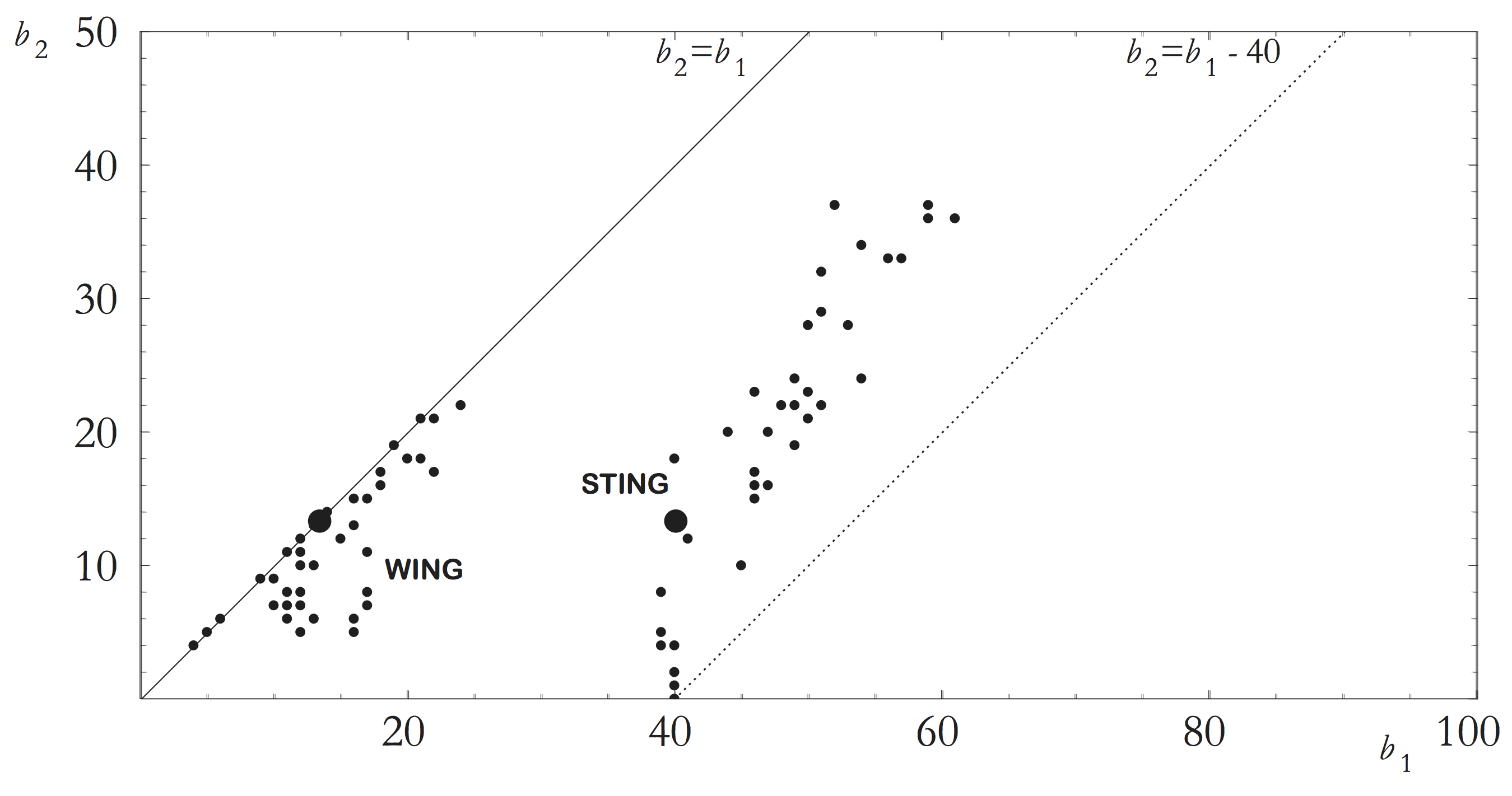
Figure 1 reports the set of options (or contracts) used in the experiment. As Figure 1 shows, contract payoffs are not distributed uniformly. Instead, they are condensed in two “clouds”, one (the WING contracts, using CABRA terminology) in which the difference in payoffs, , is relatively small; another (the STING contracts) in which player 1 is paid substantially more. These two clouds consist of contracts which are the solutions of two different mechanism design problems aimed at inducing both players to make effort. The two mechanism design problems differ in that:
- under the WING solution a player has a strict incentive to make effort only if the other does it as well;
- under the STING solution player 1’s payoff is sufficiently high to provide her with a strict incentive to make effort independently of what player 2 does, while player 2, as in the WING solution, has a strict incentive to make effort only if player 1 does it as well.
This implies that, under the STING solution, the all-effort profile is the unique Nash equilibrium of the induced game, while under the WING solution the all-no effort profile is also an equilibrium. In other words, STING contracts are strategically more robust at the expense of inducing higher payoff inequality across team members. This may create problems when players hold social (e.g., inequity averse) preferences.
The two bigger dots of Figure 1 identify optimal WING and STING contracts with “selfish” preferences, i.e., when (see Equation (3) below). All other payoff pairs are optimal when players hold some specific social preference parametrization. Notice that the difference in payoffs is bounded above (by 40). This has important consequences for the strategic analysis of the effort game, as we discuss in Section 3.
2.3. Phases
Subjects play three phases, to of increasing complexity, for a total of 72 rounds (24 rounds per phase).5 For the purpose of this paper, we only consider evidence from and .
2.3.1. Dictator Game (24 Rounds)
In we employ a variant of the classic Dictator Game. The timing for each round t and matching group is as follows.
- At the beginning of the round, a random assignment generates six pairs. Within each pair, another (independent and uniformly distributed) random device determines player position (i.e., the identity of the best paid player).
- Both players are informed about the round choice set, , and select their preferred option.
- Another independent draw fixes the identity of the Dictator. The Dictator’s choice, k, determines monetary payoffs for that pair and round: .
2.3.2. Effort Game (24 Rounds)
Stages 1 to 3 are identical to those of Instead of stage 4, we have
- The option selected by the (randomly selected) Dictator, k, yields a 2 × 2 effort game, (see Section 3 below).
- Subjects play and their strategy profile determines their financial rewards (1).
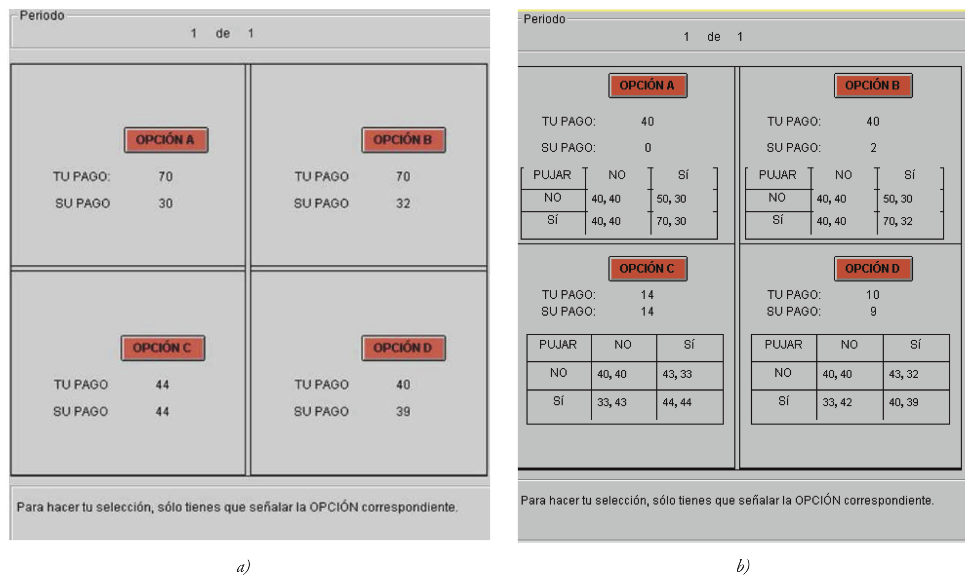
Snapshots of the user interfaces for and are shown in Panels (a) and (b) of Figure 2.
3. Theory
3.1. Game-Form
The rules of are as follows. Each player has to decide, simultaneously and independently, whether to make a costly effort. We denote by the effort decision of player where (0) if i does (not) make effort. Let denote players’ strategy profile. Player i’s monetary payoff, , is described by
with
where B is a fixed monetary prize independent of effort decision, c is the cost of effort and .6 By (2), players receive their full payoff, if they both coordinate on the effort decision, and a fixed share of the latter if only one makes effort. If nobody makes effort (i.e., if both players just earn B. In the experiment we fix and
3.2. Preferences
In what follows, i and j identify our subjects matched in pairs, and we drop the round index, whenever this does not create any ambiguity. Subjects’ social preferences are framed by way of the classic model of F&S.
Definition 1
(F&S Preferences).
where α and β identify the distributional preferences if player i, where the values of α and β determine the Dictator’s envy (i.e., aversion to inequality when receiving less than the Recipient) and guilt (i.e., aversion to inequality when receiving more than the Recipient), respectively.
We estimate social preferences in Phase 1. Remember that, by design, random player assignment determines the identity of the best paid player, who can condition her option choice on this information. As we randomize roles across rounds, we can derive from individual estimates of both distributional parameters, and .
3.3. (Preference Dependent) Beliefs
We can now look at effort decisions in as the result of a process of expected utility maximization. From (1) and (3), we derive the expected utility of player i associated to the (no) effort decision in . Without loss of generality, we simplify calculations by setting (B is a constant prize players receive under all contingencies to avoid negative monetary payoffs in the experiment); ; ; and . In other words, we normalize the prize for player 1 to be one, and rescale all other monetary payoffs accordingly. With a slight abuse of notation, let denote the expected payoff of player i of effort decision conditional on the subjective beliefs i holds over the likelihood of j to exert effort, :
In the Appendix A we model the probability of i exerting effort, , as a logistic function of the expected payoff difference . This, in turn, is a function of (a) the distributional parameters, and ; (b) the distinguishing features of the ruling contract, , and (c) the subjective beliefs of player i, , which we also model as a logistic function of—among others—the distributional parameters and . This is how we implement our proposed causality from preferences to beliefs. In other words, by our two-stage estimation approach, we can identify the direct effect of and (via their impact on the utility estimated in ), from the indirect one (via their impact on beliefs) estimated in .
For a “selfish” player (i.e., with ), an increase in is always welfare enhancing because it reduces, ceteris paribus, the probability of the no-effort outcome. This is different if players hold social preferences, because in that case the payoff difference also matters. In this respect, notice that, by (5), if your teammate free-rides on your effort, this generates envy, independently of your player position. By the same token, by (4), free-riding on your teammate’s effort always generates guilt. This is because, by construction (see Figure 1 and the discussion therein). We can generate qualitative predictions on how the expected payoff difference reacts to changes in . In this respect, Proposition 1 shows that (a) the impact of envy is reduced when increases, because this reduces the (absolute) payoff difference when i is getting less than her teammate while (b) with guilt the opposite occurs.
Proposition 1.
If λ increases, expected guilt (envy) increases (decreases), respectively.
Proof.
Let be the expected (absolute) payoff difference, conditional on the latter being positive, and the derivative of with respect to . In other words, if increases, the “expected guilt” of player 1 also increases.
By the same token, we have
- whenever , which is always the case for the contracts used in the experiment. ☐
To summarize, we have just shown that pessimistic (optimistic) beliefs on behalf of guilty (envious) players are welfare enhancing, in that they reduce the expected payoff difference in their (dis)advantage. We next check whether we can empirically establish a link between preferences and beliefs, that is, whether our estimated social preferences in Phase 1 are significant determinants of the estimated beliefs in Phase 2 and, if the case, in which direction. This is the main objective of the following structural estimation exercise.
4. Structural Estimations
As we discussed earlier, CABRA experimental design implements the two-stage identification strategy proposed by Manski [21], although in CABRA beliefs are modeled as functions of the game-form parameters only. In this respect, we contribute to the literature by including the distributional parameters estimated in in the set of regressors.7
4.1. Estimates
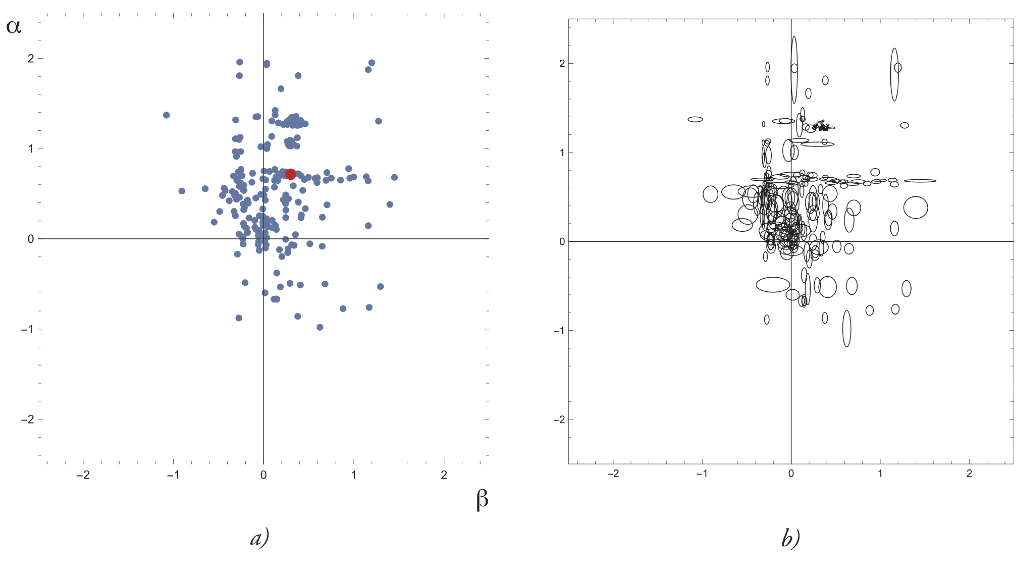
Figure 3 plots the estimated and of each participant and is composed of two graphs. In Figure 3a each subject corresponds to a point in the space. Figure 3a makes in clear that our subjects display some heterogeneity in their distributional preferences.
Figure 3b reports, together with each estimated pair (as in Figure 3a), the corresponding 95% confidence intervals associated to each individual estimated parameter pair. Social preferences of the “representative subject” (defined by the coefficients of the pool estimation) exhibit “inequity aversion” in the terminology of F&S, with both (coeff. .3, std. dev., 0.007) and (0.72, 0.015) positive and significant. As Figure 3b shows, we have many subjects whose estimated distributional preferences fall, with nonnegligible probability, in more than one quadrant. For some of them (about 50% of our subject pool), we cannot reject (at the 5% confidence level) the null hypothesis of Egoistic Preferences, . The remainder cover—with few exceptions—other preference profiles of some interest in the experimental literature, namely inequity averse preferences ( and , F&S); status seeking preferences ( and , Rey-Biel [27]) and efficiency seeking preferences ( and , Engelmann and Strobel [28]).8
4.2. Estimates
Table 1 reports the estimated coefficient of four different logit specification for . The dependent variable is , the effort decision of player i in period t of Stage 2, conditional on the payoffs selected by the random Dictator. In other words, beliefs are estimated indirectly, as a component of the difference in expected payoffs.
In Models (1) and (2) we follow CABRA and condition beliefs upon the game-form characteristics only. That is, (i) the level of wages in case of joint effort, MyB (corresonding to ) and HerB (corresponding to ), (ii) player position assignment, where Player 2 is a dummy variable positive if the decision-maker is player 2 and (iii), the contract type (either WING or STING, see Figure 1). Our estimates of Model (1) confirm the findings of CABRA in that player i is expecting more effort from j (a) the higher is j’s payoff and (b) the lower is i’s payoff. Result (a) highlights the fact that the higher is own payoff, the higher the opportunity cost of shirking. Both effects are highly significant only when we omit the other structural parameters, Pl. 2 and STING. Models (3) and (4) augment the set of regressors to the distributional parameters estimated in Phase 1, and , depending on whether player and STING dummies are included within the set of covariates. As Table 1 shows, the impact of () is always significant and positive (negative) in all models. This implies that higher envy (guilt) is associated with a significant shift of beliefs, which goes in the direction of decreasing the expected difference, as we discussed in Section 3. In the case of , this effect is nonlinear, as the coefficient of is negative and significant.
5. Discussion
It is well established stylized fact that the market for sports gambling is structured very differently from typical financial markets, despite some straightforward similarities (Levitt [29]). One peculiarity of betting markets is that individuals seldom bet against their favorite team (or preferred candidate) avoiding, so to speak, emotional hedging. This is possibly because “people do not like to anticipate undesirable outcomes and may engage in various motivated processes that lead to inflate estimates of the likelihood of desirable outcomes...” (Morewedge et al. [30], p. 2). This paper extends this simple idea to strategic situations and looks at empirical implications of a testable conjecture by which tastes and emotions affect the way in which people form beliefs about others. This approach reverses the order of causality at the core of PGT. We do not impose this reverse causality, but simply estimate it using a structural model which is especially tailored to our experimental design. The specific model of social preferences we use, namely F&S, pairs well with CABRA experimental design, in that, in Phase 1, envy and guilt can be identified. Subjects choose among alternative options after being informed about their player position, which is randomized across rounds.9 Our results suggest that social preferences according to F&S are significant in explaining subjects’ heterogeneity in beliefs in the expected direction.
A quantitative assessment on the causality between preference and beliefs is well beyond the scope of this paper (like it is, so far, also for the PGT literature that—exactly as in our case—simply assumes the reverse causality and discusses its implications). An entirely different design—in which, above all, we would also need to elicit beliefs directly—is advisable. We are well aware that belief elicitation is inherently associated with challenging design issues (incentive compatibility, to name one), which the experimental literature is well aware of since the pioneering work of Nyarko and Shotter [32].
Our analysis completely neglects any common knowledge assumption beyond these referring to the rules of the game-form. In this respect, common knowledge of rationality creates dependency of beliefs from preferences in some trivial sense (take, for example, any iterative process of deletion of dominated strategies). By contrast, PGT builds its identification strategy upon an equilibrium assumption: “we shall require that beliefs correspond to reality...” (Geanakoplos et al. [7], p. 61), which we remove completely in favor of an alternative hypothesis by which subjects hold subjective beliefs and that subjective beliefs in a game may be biased, linking this bias to subjects’ distributional concerns. Our results should be compared with those of Bellemare [33], who also look at (Ultimatum) games as individual decision problems under (strategic) uncertainty. Contrary to our approach, they elicit strategic beliefs directly and condition the estimation of social preferences a’ la F&S to beliefs (in this respect, they follow PGT in establishing causality from preferences to beliefs). Interestingly enough, they allow for a non-linear relation between payoff differences and envy and guilt and find significant evidence of a positive and concave envy, and a positive and linear guilt. Both findings are consistent with ours, conditional on our different estimation strategy.
Author Contributions
Both authors contributed equally to this work.
Funding
Financial support from the Spanish Ministry of Economic Development (ECO2015-65820-P) and Generalitat Valenciana (Grupos 3/086) is gratefully acknowledged.
Acknowledgments
This paper builds upon a long-term research project on social preferences and strategic uncertainty carried out in Alicante within the last 10 years, namely, the “CABRA project”. In this respect, we thank Antonio Cabrales, Nicola Frignani, Dunia López-Pintado, Raffaele Miniaci, Marco Piovesan, Marcello Sartarelli, Iryna Sikora, Eyal Winter and Vita Zhukova for letting us take advantage of research material from papers carried out with their direct involvement. The usual disclaimers apply.
Conflicts of Interest
The authors declare no conflict of interest. The founding sponsors had no role in the design of the study; in the collection, analyses, or interpretation of data; in the writing of the manuscript, and in the decision to publish the results.
Appendix A. Econometric Strategy
In we estimate the probability that each individual i selects his preferred option k at round t by way of the multinomial logit function
Since a random draw determines the identity of the Dictator, we model the subjects’ distributional preference parameters, and , for each participant, by maximizing the individual log-likelihood , where denotes an indicator function which is positive whenever condition is true.
We can now look at agents’ effort decisions in as the result of a process of expected utility maximization. Individual i will choose to make effort () in Stage 2 with probability
with .
In (A2) , where and denote the vectors of estimated parameters and covariates as in Table 1, respectively. Given the two-step nature of the procedure, we use datato obtain bootstrap estimates of for each of the 288 subjects, and we use them to obtain a bootstrap distribution of Step 2 estimates. Then we maximize the log-likelihood function
References
- Luce, R.D.; von Winterfeldt, D. What Common Ground Exists for Descriptive, Prescriptive, and Normative Utility Theories? Manag. Sci. 2004, 40, 263–279. [Google Scholar] [CrossRef]
- Karni, E. Probabilities and Beliefs. J. Risk Uncertain. 1996, 13, 249–262. [Google Scholar] [CrossRef]
- Kahneman, D.; Tversky, A. Prospect Theory: An Analysis of Decision under Risk. Econometrica 1979, 47, 263–291. [Google Scholar] [CrossRef]
- Tversky, A.; Kahneman, D. Advances in Prospect Theory: Cumulative Representation of Uncertainty. J. Risk Uncertain. 1992, 5, 297–323. [Google Scholar] [CrossRef]
- Antoniou, C.; Harrison, G.W.; Lau, M.; Read, D. Subjective Bayesian Beliefs. J. Risk Uncertain. 2015, 50, 35–54. [Google Scholar] [CrossRef] [Green Version]
- Prelec, D. The probability weighting function. Econometrica 1998, 66, 497–527. [Google Scholar] [CrossRef]
- Geanakoplos, J.; Pearce, D.; Stacchetti, E. Psychological Games and Sequential Rationality. Games Econ. Behav. 1989, 1, 60–79. [Google Scholar] [CrossRef]
- Battigalli, P.; Duwfenberg, M. Guilt in Games. Am. Econ. Rev. 2002, 97, 170–176. [Google Scholar] [CrossRef]
- Charness, G.; Duwfenberg, M. Promises and Partnership. Econometrica 2006, 74, 1579–1601. [Google Scholar] [CrossRef] [Green Version]
- Rabin, M. Incorporating Fairness into Game Theory and Economics. Am. Econ. Rev. 1998, 83, 1281–1302. [Google Scholar]
- Kahneman, D. New Challenges to the Rationality Assumption. J. Inst. Theor. Econ. 1994, 150, 18–36. [Google Scholar]
- Loewenstein, G.; O’Donoghue, T.; Rabin, M. Projection Bias in Predicting Future Utility. Q. J. Econ. 2003, 118, 1209–1248. [Google Scholar] [CrossRef] [Green Version]
- Dawes, R.M. Statistical criteria for establishing a truly false consensus effect. J. Exp. Soc. Psychol. 1989, 25, 1–17. [Google Scholar] [CrossRef]
- Krueger, J.I. Methodological individualism in experimental games: Not so easily dismissed. Acta Psychol. 2008, 128, 398–401. [Google Scholar] [CrossRef] [PubMed]
- Kuhlman, D.M.; Wimberley, D.L. Expectations of choice behavior held by cooperators, competitors, and individualists across four classes of experimental games. J. Pers. Soc. Psychol. 1976, 34, 69. [Google Scholar] [CrossRef]
- Ross, L.; Green, D.; House, P. The False Consensus Effect: An Egocentric Bias in Social Perception and Attribution Processes. J. Exp. Soc. Psychol. 1997, 13, 279–301. [Google Scholar] [CrossRef]
- Frey, B.; Meier, S. Social Comparisons and Pro-Social Behavior-Testing `Conditional Cooperation’ in a Field Experiment? Am. Econ. Rev. 2004, 94, 1717–1722. [Google Scholar] [CrossRef]
- Ponti, G.; Sartarelli, M.; Sikora, I.; Zhukova, V. Do Profit Opportunities and Experience Influence Principals? Efficiency? Evidence from the Lab.; Universidad de Alicante: Alicante, Spain, 2017. [Google Scholar]
- Ponti, G.; Sartarelli, M.; Sikora, I.; Zhukova, V. The Price of Entrepreneurship. Evidence from the Lab.; Universidad de Alicante: Alicante, Spain, 2018. [Google Scholar]
- Cabrales, A.; Miniaci, R.; Piovesan, M.; Ponti, G. Social Preferences and Strategic Uncertainty: An Experiment on Markets and Contracts. Am. Econ. Rev. 2010, 100, 2261–2278. [Google Scholar] [CrossRef] [Green Version]
- Manski, C.F. Identification of decision rules in experiments on simple games of proposal and response. Eur. Econ. Rev. 2002, 46, 880–891. [Google Scholar] [CrossRef]
- Fehr, E.; Schmidt, K.M. A theory of fairness,competition and cooperation. Q. J. Econ. 1999, 114, 817–868. [Google Scholar] [CrossRef]
- Fischbacher, U. z-Tree: Zurich Toolbox for Ready-made Economic Experiments. Exp. Econ. 2007, 10, 171–178. [Google Scholar] [CrossRef]
- Greiner, B. The Online Recruitment System ORSEE 2.0—A Guide for the Organization of Experiments in Economics; Working Paper Series in Economics 10; University of Cologne: Cologne, Germany, 2004; Volume 10, pp. 63–104. [Google Scholar]
- Winter, E. Incentives and Discrimination. Am. Econ. Rev. 2004, 94, 764–773. [Google Scholar] [CrossRef] [Green Version]
- Lopez-Pintado, D.; Ponti, G.; Winter, E. Inequality or Strategic Uncertainty? An Experimental Study on Incentives and Hierarchies. In Games Rationality & Behaviour; Innocenti, A., Sbriglia, P., Eds.; Palgrave Macmillan: London, UK, 2008; pp. 235–255. [Google Scholar]
- Rey-Biel, P. Inequity Aversion and Team Incentives. Scand. J. Econ. 2008, 108, 297–320. [Google Scholar]
- Engelmann, D.; Strobel, M. Inequality Aversion Efficiency and Maximum Preferences in Simple Distribution Experiments. Am. Econ. Rev. 2004, 94, 857–869. [Google Scholar] [CrossRef]
- Levitt, S.D. Why are gambling markets organized so differently from financial markets? Econ. J. 2004, 114, 223–246. [Google Scholar] [CrossRef]
- Morewedge, C.K.; Tang, S.; Larrick, R.P. Betting Your Favorite to Win: Costly Reluctance to Hedge Desired Outcomes. Manag. Sci. 2016. [Google Scholar] [CrossRef]
- Frignani, N.; Ponti, G. Risk versus social preferences under the veil of ignorance. Econ. Lett. 2012, 116, 143–146. [Google Scholar] [CrossRef]
- Nyarko, Y.; Schotter, A. An Experimental Study of Belief Learning Using Elicited Beliefs. Econometrica 2002, 70, 971–1005. [Google Scholar] [CrossRef] [Green Version]
- Bellemare, C.; Kröger, S.; van Soest, A. Actions and Beliefs: Estimating Distribution-Based Preferences Using a Large Scale Experiment with Probability Questions on Expectations. Econometrica 2008, 76, 815–839. [Google Scholar] [CrossRef]
| 1 | See also Karni [2], for a similar view. |
| 2 | A similar conjecture is supported by the so-called social projection theory (take, e.g., Dawes [13], Krueger [14] and Kuhlman et al. [15]). See also the the analysis of the so-called false consensus bias proposed by Ross et al. [16] and Frey and Meier [17], by which actions—rather than preferences—influence beliefs. |
| 3 | The experiment was programmed and conducted with the software z-Tree (Fischbacher [23]). The interested reader can find in CABRA a more detailed account of the design of Phases 1 and 2, including the experimental instructions. |
| 4 | Participants gave their informed consent to participate in the experiment at the moment of signing up in the recruiting platform ORSEE (Greiner [24]). |
| 5 | A new set of instructions was distributed at the beginning of each phase. In this sense, subjects were not aware at all times about the rules of the phases that would come next. |
| 6 | |
| 7 | A more detailed account of our estimation strategy can be found in the Appendix A. |
| 8 | No consistent version of social preferences can rationalize subjects with and , who can be then characterized as “noisy players”. |
| 9 | Frignani and Ponti [31] also apply the CABRA experimental design and analyze a situation in which make their option under the veil of ignorance, that is, before they are informed about the player position assignment. |
Figure 1.
The contract set (source: CABRA).

Figure 2.
User interface for the distributional decisions of (a) and (b) .

Figure 3.
Individual estimates of and . (a) plots the individual estimated (, ) pair; (b) reports the corresponding 95% confidence intervals associated to each individual estimated parameter pair.
Figure 3.
Individual estimates of and . (a) plots the individual estimated (, ) pair; (b) reports the corresponding 95% confidence intervals associated to each individual estimated parameter pair.


Table 1.
Structural estimations.
| Lambda | (1) | (2) | (3) | (4) |
|---|---|---|---|---|
| Myb | –0.071 *** | –0.001 | –0.102 *** | –0.091 *** |
| (0.005) | (0.027) | (0.005) | (0.0118) | |
| Herb | 0.022 *** | –0.014 | 0.034 *** | 0.031 *** |
| (0.004) | (0.015) | (0.003) | (0.007) | |
| Pl. 2 | 0.108 | –0.041 | ||
| (0.070) | (0.041) | |||
| STING | –2.602 *** | –0.603 | ||
| (0.950) | (0.463) | |||
| Pl. 2 × STING | 2.762 *** | 0.550 | ||
| (1.050) | (0.483) | |||
| 2.444 *** | 2.429 *** | |||
| (0.287) | (0.276) | |||
| –0.898 *** | –0.899 *** | |||
| (0.245) | (0.240) | |||
| –0.610 *** | –0.645 *** | |||
| (0.212) | (0.218) | |||
| –0.126 | –0.108 | |||
| (0.110) | (0.111) | |||
| cons. | 0.482 *** | –0.029 | 1.016 *** | 0.972 *** |
| (0.072) | (0.220) | (0.145) | (0.157) | |
| LogLik | –8197.051 | –8098.377 | –6534.9277 | –6504.0093 |
Std. err. in parentheses—*** p < 0.01.
© 2018 by the authors. Licensee MDPI, Basel, Switzerland. This article is an open access article distributed under the terms and conditions of the Creative Commons Attribution (CC BY) license (http://creativecommons.org/licenses/by/4.0/).
Share and Cite
MDPI and ACS Style
Giaccherini, M.; Ponti, G. Preference Based Subjective Beliefs. Games 2018, 9, 50. https://doi.org/10.3390/g9030050
AMA Style
Giaccherini M, Ponti G. Preference Based Subjective Beliefs. Games. 2018; 9(3):50. https://doi.org/10.3390/g9030050
Chicago/Turabian StyleGiaccherini, Matilde, and Giovanni Ponti. 2018. "Preference Based Subjective Beliefs" Games 9, no. 3: 50. https://doi.org/10.3390/g9030050
Note that from the first issue of 2016, this journal uses article numbers instead of page numbers. See further details here.