Optimal Control of Heterogeneous Mutating Viruses

Abstract

Different strains of influenza viruses spread in human populations during every epidemic season. As the size of an infected population increases, the virus can mutate itself and grow in strength. The traditional epidemic SIR model does not capture virus mutations and, hence, the model is not sufficient to study epidemics where the virus mutates at the same time as it spreads. In this work, we establish a novel framework to study the epidemic process with mutations of influenza viruses, which couples the SIR model with replicator dynamics used for describing virus mutations. We formulated an optimal control problem to study the optimal strategies for medical treatment and quarantine decisions. We obtained structural results for the optimal strategies and used numerical examples to corroborate our results.

1. Introduction

An epidemic of infectious disease occurs when a virus population undergoes genetic mutations or new species of viruses are introduced into the host population, and host immunity to that change in the virus population is suddenly reduced below a certain threshold. Hence, epidemic modeling should take into account not only the population dynamics of the host population, but also those of the viruses. In traditional epidemiological models, differential equations are used to capture the dynamic evolution of different classes of host populations. In particular, susceptible (S) is the class of people who are not infected; infected (I) is the class of people who have the disease; and removed or recovered (R) represents the quarantined or immune population. The commonly used SIR model [1,2] is used to describe the population migrations between these three classes of models. In order to capture the interdependencies between a virus and host populations, we established a system framework that combines the SIR model with evolutionary models that describe virus mutations.

In this work, we studied an influenza epidemic in urban populations. We analyzed the evolutionary model for virus mutations together with SIR models for the evolution of susceptible, infected, and recovered subpopulations. Over the time, individuals from these subpopulations randomly interact with each other and change their state. We consider the epidemic process as a dynamic process of changing states from susceptible individuals to the infected and finally to the recovered. The influenza epidemic is a fast-spreading process, involving a large part of the total population. Hence, one key concern is protecting a population during the annual epidemic season. There exist methods of prevention that reduce the sickness rate to protect populations, and medical measures (pharmacological products, quarantine policies, etc.) that reduce the number of the infected in the population.

Another aspect of the influenza epidemic is that different strains of influenza viruses can spread in the population during each epidemic season. As it was shown in previous studies, influenza viruses have many modifications and can quickly transform every season. Thus, by including a simulation of the mutation process into the SIR model, we can preliminarily forecast treatment strategies. In this work, we used evolutionary-game tools to describe the evolution of the influenza virus because this approach allows us to estimate the survivability of virus modifications and to determine the strongest modification. Thereby, we can use treatment strategies more effectively.

More specifically, in our work, we assume that the virus has two types with different strains and fitness functions. Both types of viruses spread in urban populations, and, hence, during an epidemic, different parts of population are infected. In our model, we split infected subpopulations into two subgroups and considered a modified SIR model. Therefore, the epidemic process in urban population depends on changes in the virus population.

In our work, we formulated the SIR model under the mechanism of a virus mutation that affects a human population and considered the minimization of treatment costs and the number of infected in both subpopulations to reduce the speed of epidemics. This complex problem is formulated as an optimal-control problem, and the virus mutation is described by replicator dynamics.

The paper is organized as follows. In Section 2, we discuss related work to our model. Section 3 presents the evolutionary model of viruses. In Section 4, we establish the epidemic model for urban populations. In Section 5, we use Pontryagin’s maximum principle to find the optimal control and present structural results of the optimal-control problem. In Section 6, we used a numerical simulation to illustrate our results. The paper is concluded in Section 7.

2. Related Works

The recent literature has seen a surge of interest in using optimal control and game-theoretic methods to study disease control of influenza for public health [3,4,5]. This research problem can be traced back to Reference [6], where an SIR type of mathematical framework was proposed to study epidemic spread in a homogeneous population. It provides a deterministic dynamical system model as the mean field approximation of the underlying stochastic evolution of the host subpopulations. In Reference [7], a control problem was formulated for a model of the carrier-borne epidemic model, and it was shown that the optimal-control effort switches at maximum once between the maximum and the minimum control effort. In Reference [8], many variants of optimal-control models of SIR epidemics were investigated for the application of medical vaccination and health-promotion campaigns. In References [9,10], a dynamic SIR epidemic model was used to identify the optimal vaccination-policy mixes for flu season.

Epidemic models have also been used in computer science and engineering to describe the temporal evolution of worm propagation in computer networks [11,12,13]. Methods such as stochastic system analysis and optimal control have been applied to provide insights on the spread of epidemics, as well as disease-control policies for protecting a population with quarantine and removal. In Reference [14], sequential hypothesis testing was adopted to detect worm-epidemic propagation over the Internet under a stochastic density-dependent Markov jump process propagation model. In References [15,16], optimal-control methods were used to study the class of epidemic models in mobile wireless networks, and Pontryagin’s maximum principle was used to quantify the damage that malware could inflict on the network by deploying optimum decision rules.

Game-theoretic approaches were also used to analyze the strategic interactions between malicious worms and the system under attack. In Reference [17], a virus-protection game was proposed based on two-state epidemic models for N nodes and the characterization of the equilibrium focus on the steady state of the response. In Reference [18], static- and dynamic-game frameworks were used to design equilibrium-revocation strategies for defending sensor networks from node-capturing and cloning attacks. It was shown that the $N+1$ non-zero-sum differential game framework was equivalent to a zero-sum differential game between a team of N attackers and the system. In References [19,20] the SIR model was combined with a game-theoretical approach to define the optimal medical approach: vaccination or treatment of seasonal influenza.

In many modern studies, different modifications of SIR models were used to estimate the behavior of infectious diseases, such as Ebola and Severe acute respiratory syndrome (SARS) [21].

Different from past works, this paper considers a coupled system framework composed of the SIR epidemic model and the evolutionary dynamic model for virus mutations. This framework is motivated by the fact that the epidemic spread of a virus can facilitate virus mutations, strengthening its virulence, which, in turn, expedites the spread and worsens epidemics. The SIR epidemic model with virus mutations can capture this complex interactions between virus and host, and allows us to explain more complex phenomena through analysis.

3. Evolutionary Model of Virus Mutations

Infectious diseases, such as influenza and SARS, are urgent public health problems in modern urban environments. Influenza spreads faster, especially in large urban populations, and affects people’s lifestyle and working facilities. The occurrence of epidemics depends on many factors, such as the size of the human population, and the virus strain and virulence, and it has become important to use effective tools to reduce their influence on human populations [22,23,24]. A mathematical model of virus infections in a population can be used to study the factors that influence epidemic growth to improve existing treatments and evaluate new effective prevention measures and treatment. In earlier research in the literature, it was shown that, during epidemic season, the influenza virus can mutate, and several types of the influenza virus circulate in the human population. Different mutations of the influenza virus affect human beings with different intensities, and epidemics evolve depending on virus type and intensity. Hence, the evolution of virus mutations should be taken into account when the SIR model is used to model influenza epidemics.

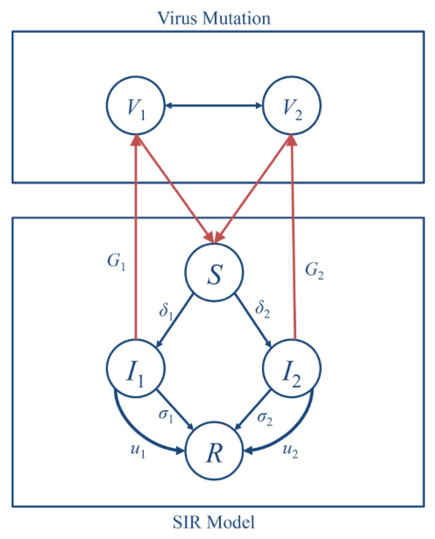
In this work, we coupled together two dynamic processes, i.e., the evolution of virus mutations and the epidemic process in human populations, as one dynamical system. The corresponding scheme of the system is illustrated in Figure 1. At the top level, two different types of the influenza virus compete to infect the host to continue their life cycles, and thereby lead to the spread of epidemics in the human population. The total population would contain several infected subpopulations that correspond to different virus types. On the bottom level, the human population is divided into subpopulations: the susceptible (S), the infected (I), and the recovered (R).

Spreading of viruses can be controlled using prevention measures such as medical treatment or isolation of infected individuals of population. Thus, at this level, we considered the SIR model with those control parameters.

At the top level of coupled dynamical system, we used evolutionary dynamics to describe the mutations within the virus population. We first describe the interactions between two virus types using an evolutionary-game model, for which we defined pure strategies, fitness, and rule of changes in a population. In the game, two types of viruses compete for human organisms, and, depending on the strength of the virus, one type can survive or vanish from the virus population.

We assume that the virus has two types or strains, denoted by $V_1$ and $V_2$, and without loss of generality, we assume that $V_2$ dominates virus $V_1$. The fitness of virus type $V_i$ in the population is ${\overline{J}}_i(V_i,V_j),i,j=1,2$, which depends on the survivability of the virus among its infected population (e.g., human beings). The life cycle of viruses requires a host organism, and occupation of such an organism leads to energy costs. Hence, virus payoff ${\overline{J}}_i$ is composed of two components: one is the utility of occupying the host organism, and the other is the cost, i.e., energy costs, ${\overline{J}}_i=b_i-C_i$, $b_i>0$, $C_i>0$, $b_i<C_i$, $C_2<C_1.$ Utility of occupation $b_i=b\left(I_i\right)$, as well as energy costs $C_I=C\left(I_i\right)$, are the functions of population state $I_i$ and, hence, mixed strategies $x_1,x_2\in [0,1]$ over set $(V_1,V_2)$ are also dependent on the population states. Here, a mixed strategy is defined as the fraction of corresponding virus types circulating in a population. Thereby, the state of the virus population is defined as value $x\left(t\right)=(x_1\left(t\right),x_2\left(t\right))$, where $x_1\left(t\right)+x_2\left(t\right)=1,\forall t\in [0,T]$.

Depending on virus strength, the number of people infected by different virus types is different. We used two flows of epidemic processes in a human population to describe our model and the population. We used $I_1$ to denote the population state for the subpopulation infected by the Type 1 virus, and $I_2$ is the state for the subpopulation infected by the Type 2 virus. Both viruses spread over the entire human population, and the interactions between two viruses when attacking the same human organism are described with the following four scenarios:

• if virus $V_1$ meets virus $V_1$, then utility for both is equal to $\frac{b_1-C_1}{2}$. The virus incurs energy costs $C_1$ with probability $1/2$ if it cannot occupy a host organism, and achieves utility of $b_1$ with probability $1/2$ if it succeeds in occupation.
• if virus $V_1$ competes with virus $V_2$, then virus $V_1$ obtains utility of 0, and $V_2$ obtains a payoff of $b_2$.
• if virus $V_2$ meets $V_2$, then both viruses obtain a payoff of $\frac{b_2-C_2}{2}$.

The above four competition cases between the two types of viruses are summarized in the following matrix representation:

	$V_1$	$V_2$
$V_1$	$({\displaystyle \frac{b_1-C_1}{2}},{\displaystyle \frac{b_1-C_1}{2}})$	$(0,b_2)$
$V_2$	$(b_2,0)$	$({\displaystyle \frac{b_2-C_2}{2}},{\displaystyle \frac{b_2-C_2}{2}})$.

According to the theory of evolutionary games [25], we compared the payoff of the i-th pure strategy with the average payoff of the total population. If the difference was positive, then the number of individuals using this pure strategy increases, or otherwise decreases. The average payoff of population $u:R^2\to R$ is defined as

$$u(x,x)=\sum _{i=1}^k{x}_{i}u(e^i,x),$$

where $e^i\in R^2,i=1,2,$ is a vector with i-th element being one and 0 otherwise, indicating the i-th pure strategy; u is a continuous function. The payoff of the i-th pure strategy is defined by $u(e^i,x)=e^{i}Ax,$ where A is the payoff matrix of the current symmetric game, and $x_i\left(t\right)$ is a fraction of virus $V_i$ [26].

To describe the evolution of the virus, we need to use a system of differential equations. In the current work, we focused on replicator dynamics [27] to describe changes of states in virus populations.

$${\dot{x}}_i=\epsilon [u(e^i,x)-u(x,x)]x_i,$$

(1)

where $\epsilon \in R_{+}$ is the time-scaling factor. Since the mutation process in a virus population and the epidemic process in a human population may develop with different speeds (e.g., virus can mutate faster than spread in human populations), $\epsilon$ can be used to describe such difference in the time scale of the two dynamics.

The stationary state of System of differential Equation (1) leads to a symmetric Nash equilibrium [26,27]. Therefore, depending on parameters $b_i$ and $C_i$, the game has two asymmetric Nash equilibria $(1,0)$, $(0,1)$ corresponding to the strategies in which all populations are types $V_1$ and $V_2$, respectively; and one symmetric Nash equilibrium $(\overline{x},\overline{x})$, where $\overline{x}=({\overline{x}}_1,{\overline{x}}_2)$, ${\overline{x}}_1=\frac{a_2}{a_1+a_2},{\overline{x}}_2=\frac{a_1}{a_1+a_2}$, here $a_1=\frac{b_1-C_1}{2}-b_2$, $a_2=\frac{b_2-C_2}{2}$. The symmetric case is more interesting since both virus types have influence on the human population. By using the evolutionary scenario of virus behaviors, we can predict which type of virus will prevail in a human population. Hence, this knowledge can correct treatment therapy and, at the same time, decrease the total cost of epidemics.

4. Epidemic Process for an Urban Population

Consider a total urban population of size N with two types of viruses circulating in the population during epidemic season. The human population is divided into four groups: the susceptible, the infected by virus $V_1$, the infected by virus $V_2$, and the recovered. The susceptible are a subpopulation of human beings that are not infected by viruses but could be infected by one or both types of viruses, and they do not have immunity to them. We assume that, in human populations, two types of viruses coexist at the same time. Human organisms can be occupied by both types of viruses, and, hence, this leads to competition between viruses for the host. Depending on virus strength, we observed that the number of people infected by virus i or by virus j can be different, and people infected by virus $V_1$ or $V_2$ belong to the infected subpopulation. The recovered subpopulation consists of people recovered from being infected. The mixing of urban populations allows viruses to spread quickly, and each person in the population is assumed to be in contact with others with equal probability. Hence, when an infected individual interacts with a susceptible one, the virus spreading is made possible. A virus with higher virulence, by our assumption, has a higher probability of success in spreading when interaction occurs between an infected individual and a susceptible individual.

4.1. Epidemic Dynamics

We modeled a virus spreading in an urban population using the epidemiological SIR model, where a system of differential equations is used to describe the fraction of the urban population as a function of time. Then, at time t, $n_S\left(t\right)$, $n_{I_1}\left(t\right)$, $n_{I_2}\left(t\right)$, $n_R\left(t\right)$ correspond to fractions of the population who are susceptible, infected by virus $V_1$, infected by virus $V_2$, and recovered, respectively; for all t, condition $N=n_S+n_{I_1}+n_{I_2}+n_R$ is justified. Define $S\left(t\right)=\frac{n_S\left(t\right)}{N},I_1\left(t\right)=\frac{n_{I_1}\left(t\right)}{N}$, $I_2\left(t\right)=\frac{n_{I_2}\left(t\right)}{N}$, $R\left(t\right)=\frac{n_R\left(t\right)}{N}$, $(R\left(t\right)=1-S\left(t\right)-I_1\left(t\right)-I_2\left(t\right))$ as portions of the susceptible, the infected and the recovered in the population. At the beginning of epidemic process $t=0$, most people in the population belong to the Susceptible subpopulation, a small group in the total population is infected, and the other people are in the recovered subpopulation. Hence, the initial states are: $0<S\left(0\right)=S^0<1$, $0<I_1\left(0\right)=I_1^0<1$, $0<I_2\left(0\right)=I_2^0<1$, $R\left(0\right)=1-S^0-I_1^0-I_2^0.$

We extended the simple SIR model introduced by References [6,28] to describe the situation with two virus types:

$$\begin{array}{c}{\displaystyle \frac{dS}{dt}=-{\delta }_{1}S\left(t\right)I_1\left(t\right)-{\delta }_{2}S\left(t\right)I_2\left(t\right);}\hfill \\ {\displaystyle \frac{d{I}_1}{dt}=({\delta }_{1}S\left(t\right)-{\sigma }_1-u_1\left(t\right))I_1\left(t\right);}\hfill \\ {\displaystyle \frac{d{I}_2}{dt}=({\delta }_{2}S\left(t\right)-{\sigma }_2-u_2\left(t\right))I_2\left(t\right);}\hfill \\ {\displaystyle \frac{dR}{dt}=({\sigma }_1+u_1\left(t\right))I_1\left(t\right)+({\sigma }_2+u_2\left(t\right))I_2\left(t\right);}\hfill \end{array}$$

(2)

where ${\delta }_i$ are the infection rates for virus $V_i$, $i=1,2$, We can interpret self-recovery rate ${\sigma }_1$ for virus $V_1$ or ${\sigma }_2$ for virus $V_2$, which shows the probability that infected nodes from subgroups $I_1$ or $I_2$ are recovered from the infection without causing any costs to our system. Infection rate is defined as the product of infection transmissibility, i.e., the probability of infection being transmitted during contact:

$${\delta }_i\left(t\right)={\delta }_i(t-\mathsf{\Delta }t)+{\delta }_i(t-\mathsf{\Delta }t)(I_i\left(t\right)-I_i(t-\mathsf{\Delta }t)),$$

(3)

where ${\delta }_i\left(0\right)={\delta }_{i_0}{I}_i\left(0\right).$ Here ${\delta }_{i_0},i=1,2$ determine the virulence of the particular virus or the ability to infect a susceptible host.

In this work, changes in the virus population influence the parameters of the SIR model; therefore, the number of infected is a function of corresponding virus subpopulation $x_i$, $I_i\left(t\right)=I_i(x_i,t),i=1,2$. We let $I_i(x_i,t)$ be linear and ${\delta }_i\left(t\right)$ take the following form:

$${\delta }_i\left(t\right)={\delta }_i(t-\mathsf{\Delta }t)+{\delta }_i(t-\mathsf{\Delta }t)(I_i(x_i,t)-I_i(x_i,t-\mathsf{\Delta }t)).$$

Then, the SIR model can be rewritten as follows:

$$\begin{array}{c}{\displaystyle \frac{dS}{dt}=-{\delta }_1\left(t\right)S\left(t\right)-{\delta }_{2}S\left(t\right);}\hfill \\ {\displaystyle \frac{d{I}_1}{dt}={\delta }_1\left(t\right)S\left(t\right)-{\sigma }_1{I}_1\left(t\right)-u_1\left(t\right)I_1\left(t\right);}\hfill \\ {\displaystyle \frac{d{I}_2}{dt}={\delta }_2\left(t\right)S\left(t\right)-{\sigma }_2{I}_2\left(t\right)-u_2\left(t\right)I_2\left(t\right);}\hfill \\ {\displaystyle \frac{dR}{dt}=({\sigma }_1+u_1\left(t\right))I_1\left(t\right)+({\sigma }_2+u_2\left(t\right))I_2\left(t\right).}\hfill \end{array}$$

(4)

In the model above, the infection rate is captured in the evolution of the mutation process in the urban population. Medical treatment or quarantine isolation reduces the number of infected individuals in the urban population. These prevention measures can be interpreted as control parameters in the system defined as $u=(u_1,u_2)$; here, $u_i$ are fractions of the infected that are quarantined or under intensive medical treatment: $0\le u_1\left(t\right)\le 1$, $0\le u_2\left(t\right)\le 1,forallt$.

4.2. Objective Function

In this work, we minimize overall cost in time interval $[0,T]$. At any given t, the following costs exist in the system: $f_1\left(I_1\left(t\right)\right),f_2\left(I_2\left(t\right)\right)$, infected costs; $g\left(R\right(t\left)\right)$, benefit rate; $h_1\left(u_1\left(t\right)\right),h_2\left(u_2\left(t\right)\right)$, costs for medical treatments (i.e., quarantine or removal) that help reduce the epidemic spread; $k_{I_1}$, $k_{I_1}$, $k_R$, costs and benefit for invective and recovered at the end of the epidemic. Here, functions $f_i\left(I_i\right)$ are non-decreasing and twice-differentiable, convex functions, i.e., $f_i\left(0\right)=0$, $f_i\left(I_i\right)>0$ for $I_i>0,i=1,2.$, $g\left(R\right)$ is non-decreasing and differentiable function and $g\left(0\right)=0$, $h_i\left(u_i\left(t\right)\right)$ is twice-differentiable and increasing function in $u_i\left(t\right)$ such as $h_i\left(0\right)=0$, $h_i\left(u_i\left(t\right)\right)>0,i=1,2,$ when $u_i\left(t\right)>0$. We show the structure of the optimal control strategies for the general case of costs functions. Hence, in particular cases this conditions will be satisfied for any functions with the same properties.

The cost for the aggregated system is given by

$$\begin{array}{c}J={\int }_0^T{f}_1\left(I_1\left(t\right)\right)+f_2\left(I_2\left(t\right)\right)-g\left(R\left(t\right)\right)+h_1\left(u_1\left(t\right)\right)+h_2\left(u_2\left(t\right)\right)dt+\\ k_{I_1}{I}_1\left(T\right)+k_{I_1}{I}_2\left(T\right)-k_{R}R\left(T\right),\end{array}$$

(5)

and the optimal-control problem is to minimize the cost, i.e., ${min}_{\{u_1,u_2\}}J.$ To simplify the analysis, we consider the case where $k_{I_1}=k_{I_1}=k_R=0$.

5. Optimal Control of Epidemics

We used Pontryagin’s maximum principle [29] to find optimal control $u\left(t\right)=(u_1\left(t\right),u_2\left(t\right))$ to the problem described in Section 4 above. Define associated Hamiltonian H and adjoint functions ${\lambda }_S$, ${\lambda }_{I_1}$, ${\lambda }_{I_2}$, ${\lambda }_R$ as follows:

$$\begin{array}{cc}\hfill H=& f_1\left(I_1\left(t\right)\right)+f_2\left(I_2\left(t\right)\right)-g\left(R\left(t\right)\right)+h_1\left(u_1\left(t\right)\right)+h_2\left(u_2\left(t\right)\right)+\hfill \\ & ({\lambda }_{I_1}-{\lambda }_S){\delta }_{1}S{I}_1+({\lambda }_{I_2}-{\lambda }_S){\delta }_{2}S{I}_2+({\lambda }_R-{\lambda }_{I_1}){\sigma }_1{I}_1+\hfill \\ & ({\lambda }_R-{\lambda }_{I_2}){\sigma }_2{I}_2-({\lambda }_{I_1}-{\lambda }_R)I_1{u}_1-({\lambda }_{I_2}-{\lambda }_R)I_2{u}_2.\hfill \end{array}$$

(6)

Here, we used condition $R\left(t\right)=1-S\left(t\right)-I_1\left(t\right)-I_2\left(t\right)$. We constructed an adjoint system as follows:

$$\begin{array}{l}{\dot{\lambda }}_S\left(t\right)=-{\displaystyle \frac{\partial H}{\partial S}}=-{\lambda }_S(-{\delta }_1{I}_1-{\delta }_2{I}_2)-{\lambda }_{I_1}{\delta }_1{I}_1;\hfill \\ {\dot{\lambda }}_{I_1}\left(t\right)=-{\displaystyle \frac{\partial H}{\partial I_1}}=-f_1^{\prime }\left(I_1\right)+{\lambda }_S{\delta }_{1}S-{\lambda }_{I_1}({\delta }_{1}S-{\sigma }_1)-{\lambda }_R{\sigma }_1;\hfill \\ {\dot{\lambda }}_{I_2}\left(t\right)=-{\displaystyle \frac{\partial H}{\partial I_2}}=-f_2^{\prime }\left(I_2\right)+{\lambda }_S{\delta }_{2}S-{\lambda }_{I_2}({\delta }_{2}S-{\sigma }_2)-{\lambda }_R{\sigma }_1;\hfill \\ {\dot{\lambda }}_R\left(t\right)=-{\displaystyle \frac{\partial H}{\partial R}}=\left(g^{\prime }\left(R\right)\right);\end{array}$$

(7)

with transversality conditions given by:

$${\lambda }_{I_1}\left(T\right)=0,{\lambda }_{I_2}\left(T\right)=0,{\lambda }_S\left(T\right)=0,{\lambda }_R\left(T\right)=0.$$

(8)

According to Pontryagin’s maximum principle, there exist continuous and piecewise continuously differentiable costate functions ${\lambda }_i$ that, at every point $t\in [0,T]$, where $u_1$ and $u_2$ are continuous, satisfy System (7) and Equation (8). In addition, we have:

$$(u_1,u_2)\in \arg \underset{{\overline{u}}_1,{\overline{u}}_2\in [0,1]}{min}H(\overline{\lambda },(S,I_1,I_2,R),({\overline{u}}_1,{\overline{u}}_2)).$$

(9)

5.1. Structure of Optimal Control

Based on previous research [12,16,29], in this subsection we show that optimal control $u\left(t\right)=(u_1\left(t\right),u_2\left(t\right))$ has the following structural results:

Proposition 1.

The following statements hold for the optimal-control problem described in Section 4:

• When $h_i(·)$ are concave functions, then there exist time moments $t_1\in [0,T]$, such that:

  $$u\left(t\right)=(u_1\left(t\right),u_2\left(t\right))=\left\{\begin{array}{c}(1,1),for0<t<t_1;\hfill \\ (0,0),for{t}_1<t<T.\hfill \end{array}\right.$$
• When $h_i(·)$ are strictly convex functions, then there exist time moments $t_0,t_1$, $0<t_0<t_1<T$ such that:

  $$u_i\left(t\right)=\left\{\begin{array}{c}0,{\varphi }_i\left(t\right)\le h_i^{\prime }\left(0\right),i=1,2;\hfill \\ h^{\prime -1}\left({\varphi }_i\right),h_i^{\prime }\left(0\right)<{\varphi }_i\left(t\right)\le h_i^{\prime }\left(1\right),i=1,2;\hfill \\ 1,h_i^{\prime }\left(1\right)<{\varphi }_i\left(t\right),i=1,2.\hfill \end{array}\right.$$

The proof of Proposition 1 requires auxiliary Lemma 1 and it is discussed in detail in Section 5.2. Before stating Lemma 1, we define functions ${\varphi }_i$ as follows:

$${\varphi }_1\left(t\right)=({\lambda }_{I_1}\left(t\right)-{\lambda }_R\left(t\right))I_1\left(t\right),{\varphi }_2\left(t\right)=({\lambda }_{I_2}\left(t\right)-{\lambda }_R\left(t\right))I_2\left(t\right).$$

Rewrite the Hamiltonian in terms of function $\varphi$ and we obtain:

$$\begin{array}{c}H=(f_1\left(I_1\left(t\right)\right)+f_2\left(I_2\left(t\right)\right)-g\left(R\left(t\right)\right)+({\lambda }_{I_1}-{\lambda }_S){\delta }_{1}S{I}_1+\hfill \\ ({\lambda }_{I_2}-{\lambda }_S){\delta }_{2}S{I}_2+({\lambda }_R-{\lambda }_{I_1}){\sigma }_1{I}_1+({\lambda }_R-{\lambda }_{I_2}){\sigma }_2{I}_2+\hfill \\ (h_1\left(u_1\left(t\right)\right)-{\varphi }_1{u}_1)+(h_2\left(u_2\left(t\right)\right)-{\varphi }_2{u}_2).\hfill \end{array}$$

(10)

For any admissible control ${\tilde{u}}_1,{\tilde{u}}_2$ and according to Equation (9), for all $t\in [0,T]$:

$$\begin{array}{c}[(h_1\left(u_1\left(t\right)\right)-{\varphi }_1{u}_1)+(h_2\left(u_2\left(t\right)\right)-{\varphi }_2{u}_2)]\le \hfill \\ h_1\left({\tilde{u}}_1\left(t\right)\right)-{\varphi }_1{\tilde{u}}_1)+(h_2\left({\tilde{u}}_2\left(t\right)\right)-{\varphi }_2{\tilde{u}}_2),\hfill \end{array}$$

(11)

then, we obtain

$$\begin{array}{c}(u_1\left(t\right),u_2\left(t\right))\in \arg \underset{\begin{array}{c}x\in [0,1],y\in [0,1]\hfill \end{array}}{min}(h_1\left(x\right)-{\varphi }_{1}x)+(h_2\left(y\right)-{\varphi }_{2}y).\hfill \end{array}$$

(12)

We observe that

$$\begin{array}{c}\underset{u_1,u_2}{min}[(h_1\left(u_1\left(t\right)\right)-{\varphi }_1{u}_1\left(t\right))+(h_2\left(u_2\left(t\right)\right)-{\varphi }_2{u}_2\left(t\right))]\hfill \\ =\underset{u_1}{min}(h_1\left(u_1\left(t\right)\right)-{\varphi }_1{u}_1)+\underset{u_2}{min}(h_2\left(u_2\left(t\right)\right)-{\varphi }_2{u}_2).\hfill \end{array}$$

Since $u_1=u_2=0$ are admissible control, using Equation (11), we obtain

$$\begin{array}{c}(h_1\left(u_1\left(t\right)\right)-{\varphi }_1{u}_1)+(h_2\left(u_2\left(t\right)\right)-{\varphi }_2{u}_2)\le \hfill \\ (h_1\left(0\right)-{\varphi }_{1}0)+(h_2\left(0\right)-{\varphi }_{2}0)=0,\mathrm{for}\mathrm{all}t.\hfill \end{array}$$

(13)

To prove Proposition 1, we consider the following auxiliary lemma:

Lemma 1.

Functions ${\varphi }_i,i=1,2$ are decreasing functions of t, for $t\in [t_0,T],$ $t_0\ge t\ge 0,$ while

$${\delta }_{i}S{I}_i-{\sigma }_i{I}_i\ge u_i,i=1,2.$$

(14)

Proof of Lemma 1.

The state and costate functions are differentiable functions; then, ${\varphi }_i$ are also differentiable functions at each time t, $t\in [0,T]$ at which functions $u_1,u_2$ are continuous. We have to show that $\dot{{\varphi }_i}<0$ at each time $t\in [t_0,T],$ $t_0\ge t\ge 0$. Consider function ${\varphi }_1$ given by

$$\begin{array}{c}\dot{{\varphi }_1}=-(f_1^{\prime }\left(I_1\right)-({\lambda }_{I_1}-{\lambda }_S){\delta }_{1}S-({\lambda }_R-{\lambda }_{I_1}){\sigma }_1-g^{\prime }\left(R\right))I_1-\hfill \\ ({\lambda }_R-{\lambda }_{I_1})({\delta }_{1}S{I}_1-{\sigma }_1{I}_1-I_1{u}_1),\hfill \end{array}$$

(15)

and, likewise, ${\varphi }_2$ as follows:

$$\begin{array}{c}\dot{{\varphi }_2}=-(f_2^{\prime }\left(I_2\right)-({\lambda }_{I_2}-{\lambda }_S){\delta }_{2}S-({\lambda }_R-{\lambda }_{I_2}){\sigma }_2-g^{\prime }\left(R\right))I_2-\hfill \\ ({\lambda }_R-{\lambda }_{I_1})({\delta }_{2}S{I}_2-{\sigma }_2{I}_2-I_2{u}_2).\hfill \end{array}$$

(16)

Here, $f_1^{\prime }\left(I_1\right)\ge 0$, $f_2^{\prime }\left(I_2\right)\ge 0$, $g^{\prime }\left(R\right)\ge 0$, ${\delta }_i\ge 0$, $I_1,I_2,S,R\ge 0$, then, the right-hand side of Expressions (15) and (16) are negative if conditions ${\delta }_{1}S{I}_1-{\sigma }_1{I}_1\ge u_1$ and ${\delta }_{2}S{I}_2-{\sigma }_2{I}_2\ge u_2$ are satisfied; otherwise, functions ${\varphi }_i$ are increasing. Term ${\delta }_{i}S{I}_i-{\sigma }_i{I}_i\ge u_i\ge 0$, $i=1,2$ can be interpreted as a condition for the beginning of the epidemic (see Reference [6]). The proof of Lemma 1 is completed. □

5.2. Proof of Proposition 1

In this subsection, we prove Proposition 1 under two cases of cost functions $h_i\left(u_i\right),i=1,2.$

5.2.1. $h_i$ Are Concave

Let $h_1$ and $h_2$ be concave ($h_1^{″}<0,h_2^{″}<0$); then, ($h_1\left(x\right)-{\varphi }_{1}x$) and ($h_2\left(y\right)-{\varphi }_{2}y$) are convex functions of x and y. For any time t, the unique mimimum is either in $x=0$ or $x=1$ ($y=0$ or $y=1$).

From Equation (10), we have that optimal $u_i$ satisfies $h_i\left(u_i\right)-u_i{\varphi }_i\le h_i\left({\tilde{u}}_i\right)-{\tilde{u}}_i{\varphi }_i$, where ${\tilde{u}}_i$ are any admissible control, ${\tilde{u}}_i\in [0,1]$. If $u_i=1$, then switching functions are satisfied ${\varphi }_i\ge h_i\left(1\right)$, and, if $u_i=0$, then ${\varphi }_i<h_i\left(1\right)$.

$$u_i\left(t\right)=\left\{\begin{array}{c}0,{\varphi }_i\left(t\right)<h_i\left(1\right),\hfill \\ 1,{\varphi }_i\left(t\right)\ge h_i\left(1\right).\hfill \end{array}\right.$$

(17)

Lemma 1 suggests that ${\varphi }_i$ are decreasing functions; then, there can be, at most, one time moment $t\in [0,T]$ at which ${\varphi }_i\left(t\right)=h_i^{\prime }\left(u_i\left(t\right)\right)$. Moreover, if such moment exists, for example, $t_1$, then ${\varphi }_i\left(t\right)<h_i\left(1\right)$ on $0\le t<t_1$ and ${\varphi }_i\left(t\right)\ge h_i\left(1\right)$ on $t_1\le t<T$. Then, Control (17) is satisfied.

5.2.2. $h_i(·)$ Are Convex

When $h_i(·)$ are strictly convex ($h_i^{″}>0$), then $\frac{\partial }{\partial x}(h_1\left(x\right)-{\varphi }_{1}x){\mid }_{x=x_1}=0$ and $\frac{\partial }{\partial y}(h_2\left(y\right)-{\varphi }_{1}y){\mid }_{y=y_1}=0$ at a $x\in [0,1]$ or $y\in [0,1]$, then $u_1\left(t\right)=x_1$ and $u_2\left(t\right)=y_1$, else $u_1\left(t\right)\in [0,1]$ and $u_2\left(t\right)\in [0,1]$. Then,

$$u_i\left(t\right)=\left\{\begin{array}{c}0,{\varphi }_i\left(t\right)\le h_i^{\prime }\left(0\right),i=1,2;\hfill \\ h^{\prime -1}\left({\varphi }_i\right),h_i^{\prime }\left(0\right)<{\varphi }_i\left(t\right)\le h_i^{\prime }\left(1\right),i=1,2.\hfill \\ 1,h_i^{\prime }\left(1\right)<{\varphi }_i\left(t\right),i=1,2.\hfill \end{array}\right.$$

(18)

Function ${\varphi }_i$, $h_i^{\prime }$, $u_i$ is continuous at all $t\in [0,T].$ In this case, $h_i$ is strictly convex and $h_i^{\prime }$ is a strictly increasing function, so $h^{\prime }\left(0\right)<h^{\prime }\left(1\right)$. Thus, there exist points $t_0,t_1$, $0<t_0<t_1<T$, so that Conditions (14) and (18) are satisfied; according to that, ${\varphi }_i$ is a decreasing function. In a time interval where ${\delta }_{i}S{I}_i-{\sigma }_i{I}_i<u_i,i=1,2$, functions ${\varphi }_i$ are increasing and Conditions (18) are rewritten. There may exist such time interval $[0,t_0)$ that $u_i=0$ and ${\varphi }_i\le h_i^{\prime }\left(0\right),i=1,2$; then, for time interval $[t_0,T]$, Conditions (18) continue to be satisfied.

Using auxiliary Lemma 2, we completed the proof of Proposition 1. From Lemma 1, we need to check that multipliers $({\lambda }_{I_1}\left(t\right)-{\lambda }_S\left(t\right))$, $({\lambda }_{I_2}\left(t\right)-{\lambda }_S\left(t\right))$, $({\lambda }_R\left(t\right)-{\lambda }_{I_1}\left(t\right))$ in Equations (15) and (16) are non-negative.

Lemma 2.

For all $0\le t\le T$, we have $({\lambda }_{I_1}\left(t\right)-{\lambda }_S\left(t\right))>0$, $({\lambda }_{I_2}\left(t\right)-{\lambda }_S\left(t\right))>0$ and $({\lambda }_R\left(t\right)-{\lambda }_{I_1}\left(t\right))>0$.

Property 1.

Let $w\left(t\right)$ be a continuous and piecewise differential function of t. Let $w\left(t_1\right)=L$ and $w\left(t\right)>L$ for all $t\in (t_1,\dots ,t_0]$. Then $\dot{w\left(t_1^{+}\right)\ge 0}$, where $w\left(t_1^{+}\right)=\underset{x\to x_0}{lim}v\left(x\right)$.

Property 2.

For any convex and differentiable function $y\left(x\right)$, which is 0 at $x=0$, $y^{\prime }\left(x\right)x-y\left(x\right)\ge 0$ for all $x\ge 0$.

Proof: We first prove the case for $t=T$ and then for $t<T$.

Step 1. At time T, we have $({\lambda }_{I_1}\left(T\right)-{\lambda }_S\left(T\right))=0$, $({\lambda }_{I_2}\left(T\right)-{\lambda }_S\left(T\right))=0$, and $({\lambda }_R\left(T\right)-{\lambda }_{I_1}\left(T\right))=0$ according to (8). ${\dot{\lambda }}_{I_1}\left(T\right)-{\dot{\lambda }}_S\left(T\right)=-f_1^{\prime }\left(I_1\left(T\right)\right)<0$ and by analogy ${\dot{\lambda }}_{I_2}\left(T\right)-{\dot{\lambda }}_S\left(T\right)=-f_2^{\prime }\left(I_2\left(T\right)\right)<0$ and ${\dot{\lambda }}_R\left(T\right)-{\dot{\lambda }}_{I_1\left(T\right)}=f_1^{\prime }\left(I_1\left(T\right)\right)+g\left(R\left(T\right)\right)>0$, therefore expressions $({\lambda }_{I_1}\left(T\right)-{\lambda }_S\left(T\right))$, $({\lambda }_{I_2}\left(T\right)-{\lambda }_S\left(T\right))$, $({\lambda }_R\left(T\right)-{\lambda }_S{I}_1\left(T\right))$ are positive in open interval $(0,T)$.

Step 2. (Proof by contradiction).

Let $t^{*}<T$ be the last time at which one of the inequality constraints holds:

Case I. In this case, we prove that $({\lambda }_{I_1}\left(t\right)-{\lambda }_S\left(t\right))>0.$ Suppose that $({\lambda }_{I_1}\left(t\right)-{\lambda }_S\left(t\right))=0$, $({\lambda }_{I_2}\left(t\right)-{\lambda }_S\left(t\right))=0$ and $({\lambda }_R\left(t\right)-{\lambda }_{I_1}\left(t\right))>0$ then

$$\begin{array}{c}{\dot{\lambda }}_{I_1}\left(t^{*}\right)-{\dot{\lambda }}_S\left(t^{*}\right)=f_1^{\prime }\left(I_1\right)-({\lambda }_{I_1}-{\lambda }_S){\delta }_{1}S-({\lambda }_R-{\lambda }_{I_1}){\sigma }_1-\hfill \\ ({\lambda }_S-{\lambda }_{I_1}){\delta }_1{I}_1-({\lambda }_S-{\lambda }_{I_2}){\delta }_2{I}_2,\hfill \end{array}$$

and hence we obtain that $({\dot{\lambda }}_{I_1}\left(t^{*}\right)-{\dot{\lambda }}_S\left(t^{*}\right))<0$. This contradicts Property 1 for function $({\lambda }_{I_1}\left(t^{*}\right)-{\lambda }_S\left(t^{*}\right))$, which means that $({\lambda }_{I_1}\left(t^{*}\right)-{\lambda }_S\left(t^{*}\right))>0.$

Now, let $({\lambda }_R\left(t\right)-{\lambda }_{I_1}\left(t\right))=0$ and $({\lambda }_R\left(t\right)-{\lambda }_{I_2}\left(t\right))=0$ and $({\lambda }_S\left(t\right)-{\lambda }_{I_1}\left(t\right))>0,({\lambda }_S\left(t\right)-{\lambda }_{I_2}\left(t\right))>0$.

$$\begin{array}{c}{\dot{\lambda }}_{I_1}\left(t^{*+}\right)-{\dot{\lambda }}_S\left(t^{*+}\right)=(-f_1^{\prime }\left(I_1\right)+{\lambda }_S{\delta }_{1}S-{\lambda }_{I_1}({\delta }_{1}S-{\sigma }_1)-{\lambda }_R{\sigma }_1)-\hfill \\ (-{\lambda }_S(-{\delta }_1{I}_1-{\delta }_2{I}_2)-{\lambda }_{I_1}{\delta }_1{I}_1)\hfill \\ =-f_1^{\prime }\left(I_1\right)-({\lambda }_{I_1}-{\lambda }_S){\delta }_{1}S-({\lambda }_R-{\lambda }_{I_1}){\sigma }_1+\hfill \\ ({\lambda }_{I_1}-{\lambda }_S){\delta }_1{I}_1+({\lambda }_{I_2}-{\lambda }_S){\delta }_2{I}_2\hfill \\ =-f_1^{\prime }\left(I_1\right)-({\lambda }_{I_1}-{\lambda }_S){\delta }_{1}S-({\lambda }_R-{\lambda }_{I_1}){\sigma }_1-\hfill \\ ({\lambda }_S-{\lambda }_{I_1}){\delta }_1{I}_1-({\lambda }_S-{\lambda }_{I_2}){\delta }_2{I}_2.\hfill \end{array}$$

(19)

If ${\delta }_1=0$ and ${\delta }_2=0$ and $({\lambda }_R\left(t\right)-{\lambda }_{I_1}\left(t\right))>0$ then ${\dot{\lambda }}_{I_1}\left(t^{*}\right)-{\dot{\lambda }}_S\left(t^{*}\right)<0$, this contradicts Property 1 for functions $({\lambda }_{I_1}\left(t^{*}\right)-{\lambda }_S\left(t^{*}\right))$ at time $t^{*}$, and such moment $t^{*}$ does not exist. Lemma 2 is proved in this case.

If ${\delta }_1>0$ and ${\delta }_2>0$, then the system of O.D.E. is autonomous, and hence the Hamiltonian and the control do not have the dependence of variable independent t.

$$\begin{array}{c}H(S\left(t\right),I_1\left(t\right),I_2\left(t\right),R\left(t\right),u_1\left(t\right),u_2\left(t\right),{\lambda }_S\left(t\right),{\lambda }_{I_1}\left(t\right),{\lambda }_{I_2}\left(t\right),{\lambda }_R\left(t\right))=constant.\hfill \end{array}$$

(20)

From Hamiltonian (6), we obtain

$$\begin{array}{c}H=f_1\left(I_1\left(t\right)\right)+f_2\left(I_2\left(t\right)\right)-g\left(R\left(t\right)\right)+h_1\left(u_1\left(t\right)\right)+h_2\left(u_2\left(t\right)\right)+\hfill \\ ({\lambda }_{I_1}-{\lambda }_S){\delta }_{1}S{I}_1+({\lambda }_{I_2}-{\lambda }_S){\delta }_{2}S{I}_2+({\lambda }_R-{\lambda }_{I_1}){\sigma }_1{I}_1+({\lambda }_R-{\lambda }_{I_2}){\sigma }_2{I}_2-\hfill \\ ({\lambda }_{I_1}-{\lambda }_R)I_1{u}_1-({\lambda }_{I_2}-{\lambda }_R)I_2{u}_2.\hfill \end{array}$$

(21)

Since $g\left(R\right)$ is a nondecreasing function, then $g\left(R\right(T\left)\right)\ge g\left(R\right(t\left)\right)$, and we obtain

$$\begin{array}{c}H-f_1\left(I_1\left(t\right)\right)+g(R\left(t\right)\ge f_2\left(I_2\left(t\right)\right)+h_1\left(u_1\left(t\right)\right)+h_2\left(u_2\left(t\right)\right)+\hfill \\ ({\lambda }_{I_1}-{\lambda }_S){\delta }_{1}S{I}_1+({\lambda }_{I_2}-{\lambda }_S){\delta }_{2}S{I}_2+\hfill \\ ({\lambda }_R-{\lambda }_{I_1}){\sigma }_1{I}_1+({\lambda }_R-{\lambda }_{I_2}){\sigma }_2{I}_2+\hfill \\ ({\lambda }_R-{\lambda }_{I_1})I_1{u}_1+({\lambda }_R-{\lambda }_{I_2})I_2{u}_2\ge 0.\hfill \end{array}$$

(22)

This follows from the assumptions on functions $f_1\left(I_1\right)$ and $h_1\left(u_1\right)$, $h_2\left(u_2\right)$, such that $I_1\left(T\right)>0$ then $f_1\left(I_1\right)>0$ and $u_1\left(t\right)>0$, $u_2\left(t\right)>0$; then, $h_1\left(u_1\right)\ge 0$, $h_2\left(u_2\right)\ge 0.$

From Hamiltonian (10), we have:

$$\begin{array}{c}H=(f_1\left(I_1\left(t\right)\right)+f_2\left(I_2\left(t\right)\right)-g\left(R\left(t\right)\right)+({\lambda }_{I_1}-{\lambda }_S){\delta }_{1}S{I}_1+\hfill \\ ({\lambda }_{I_2}-{\lambda }_S){\delta }_{2}S{I}_2+({\lambda }_R-{\lambda }_{I_1}){\sigma }_1{I}_1+({\lambda }_R-{\lambda }_{I_2}){\sigma }_2{I}_2\hfill \\ +(h_1\left(u_1\left(t\right)\right)-{\varphi }_1{u}_1)+(h_2\left(u_2\left(t\right)\right)-{\varphi }_2{u}_2).\hfill \end{array}$$

(23)

Therefore, we obtain

$$\begin{array}{c}{\displaystyle {\dot{\lambda }}_{I_1}\left(t\right)-{\dot{\lambda }}_S\left(t\right)=-f_1^{\prime }\left(I_1\right)+\frac{f_1\left(I_1\left(t\right)\right)+f_2\left(I_2\left(t\right)\right)-g(R\left(t\right)-H}{I_1}+}\hfill \\ {\displaystyle \frac{(h_1\left(u_1\left(t\right)\right)-{\varphi }_1{u}_1)}{I_1}+\frac{(h_2\left(u_2\left(t\right)\right)-{\varphi }_2{u}_2)}{I_1}-({\lambda }_S-{\lambda }_{I_2}){\delta }_{2}S\frac{I_2}{I_1}-}\hfill \\ {\displaystyle ({\lambda }_{I_2}-{\lambda }_R){\sigma }_2\frac{I_2}{I_1}+({\lambda }_{I_1}-{\lambda }_S){\delta }_1{I}_1+({\lambda }_{I_2}-{\lambda }_S){\delta }_2{I}_2}\hfill \\ {\displaystyle =\frac{1}{I_1}(f_1\left(I_1\right)-f_1^{\prime }\left(I_1\right)I_1)-\frac{1}{I_1}(H-f_2\left(I_2\right)+g\left(R\right))+}\hfill \\ {\displaystyle \frac{(h_1\left(u_1\left(t\right)\right)-{\varphi }_1{u}_1)}{I_1}+\frac{(h_2\left(u_2\left(t\right)\right)-{\varphi }_2{u}_2)}{I_1}-}\hfill \\ {\displaystyle ({\lambda }_S-{\lambda }_{I_2}){\delta }_{2}S\frac{I_2}{I_1}-({\lambda }_{I_2}-{\lambda }_R){\sigma }_2\frac{I_2}{I_1}-({\lambda }_S-{\lambda }_{I_1}){\delta }_1{I}_1-}\hfill \\ ({\lambda }_S-{\lambda }_{I_2}){\delta }_2{I}_2.\hfill \end{array}$$

(24)

Here, $f_1\left(I_1\right)$ is a convex increasing function and $f_1\left(0\right)=0$, $I_1>0$ and $(f_1\left(I_1\right)-f_1^{\prime }\left(I_1\right)I_1)\le 0$, by Property 2. From Transversality (8), and Lemmas (19) and (22), then ${\dot{\lambda }}_{I_1}\left(t\right)-{\dot{\lambda }}_S\left(t\right)<0$, which contradicts Property 1. Case I of the lemma follows.

Case II. We have to prove that $({\lambda }_{I_2}\left(t\right)-{\lambda }_S\left(t\right))>0$. This is a symmetric case to Case I. Using the same reasoning, we obtain

$${\displaystyle \begin{array}{c}{\dot{\lambda }}_{I_2}\left(t\right)-{\dot{\lambda }}_S\left(t\right)=-f^{\prime }\left(I_2\right)+({\lambda }_S-{\lambda }_{I_2}){\delta }_{2}S+({\lambda }_{I_2}-{\lambda }_R){\sigma }_2+({\lambda }_{I_1}-{\lambda }_S){\delta }_1{I}_1+\hfill \\ ({\lambda }_{I_2}-{\lambda }_S){\delta }_2{I}_2=\frac{1}{I_2}(f_2\left(I_2\right)-f_2^{\prime }\left(I_2\right)I_2)-\hfill \\ \frac{1}{I_2}(H-f_1\left(I_1\right)+g\left(R\right))+\frac{(h_1\left(u_1\left(t\right)\right)-{\varphi }_1{u}_1)}{I_2}+\hfill \\ \frac{(h_2\left(u_2\left(t\right)\right)-{\varphi }_2{u}_2)}{I_2}-({\lambda }_S-{\lambda }_{I_1}){\delta }_{1}S\frac{I_1}{I_2}-({\lambda }_{I_1}-{\lambda }_R){\sigma }_1\frac{I_1}{I_2}-\hfill \\ ({\lambda }_S-{\lambda }_{I_2}){\delta }_2{I}_2-({\lambda }_S-{\lambda }_{I_1}){\delta }_1{I}_1.\hfill \end{array}}$$

(25)

Thus, we have ${\dot{\lambda }}_{I_2}\left(t\right)-{\dot{\lambda }}_S\left(t\right)<0$ that contradicts Property 1, and, hence, functions $({\lambda }_{I_2}\left(t\right)-{\lambda }_S\left(t\right))>0$.

Case III. In this case, we prove that $({\lambda }_R\left(t\right)-{\lambda }_{I_1}\left(t\right))>0$ in a similar way.

$$\begin{array}{c}H-f_2\left(I_2\left(t\right)\right)+g(R\left(t\right)\ge -f_1\left(I_1\left(t\right)\right)+h_1\left(u_1\left(t\right)\right)+h_2\left(u_2\left(t\right)\right)+\hfill \\ ({\lambda }_{I_1}-{\lambda }_S){\delta }_{1}S{I}_1+({\lambda }_{I_2}-{\lambda }_S){\delta }_{2}S{I}_2+\hfill \\ ({\lambda }_R-{\lambda }_{I_1}){\sigma }_1{I}_1+({\lambda }_R-{\lambda }_{I_2}){\sigma }_2{I}_2+({\lambda }_R-{\lambda }_{I_1})I_1{u}_1+\hfill \\ ({\lambda }_R-{\lambda }_{I_2})I_2{u}_2\ge 0.\hfill \end{array}$$

(26)

This follows from the assumptions on functions $h_1\left(u_1\right)$, $h_2\left(u_2\right)$ such as $I_1\left(T\right)>0$ then $f_1\left(I_1\right)>0$ and $u_1\left(t\right)>0$, $u_2\left(t\right)>0$ then $h_1\left(u_1\right)\ge 0$, $h_2\left(u_2\right)\ge 0.$ Therefore, we obtain

$$\begin{array}{c}{\dot{\lambda }}_R\left(t\right)-{\dot{\lambda }}_{I_1}\left(t\right)=g^{\prime }\left(R\right)+f_1^{\prime }\left(I_1\right)-{\lambda }_{I_1}{\delta }_{1}S+{\lambda }_{I_2}({\delta }_{1}S-{\sigma }_1)+{\lambda }_R{\sigma }_1\hfill \\ =g^{\prime }\left(R\right)+f_1^{\prime }\left(I_1\right)+({\lambda }_{I_1}-{\lambda }_S){\delta }_{1}S+({\lambda }_R-{\lambda }_{I_1}){\sigma }_1\hfill \\ {\displaystyle =g^{\prime }\left(R\right)+f_1^{\prime }\left(I_1\right)+\frac{H}{I_1}-\frac{f_2\left(I_2\right)}{I_1}+}\hfill \\ {\displaystyle \frac{1}{I_1}(f_1^{\prime }\left(I_1\right)I_1-f_1\left(I_1\right))+\frac{g\left(R\right)}{I_1}+({\lambda }_S-{\lambda }_{I_2}){\delta }_{2}S\frac{I_2}{I_1}+}\hfill \\ {\displaystyle ({\lambda }_R-{\lambda }_{I_2}){\sigma }_2\frac{I_2}{I_1}-\frac{(h_1\left(u_1\left(t\right)\right)-{\varphi }_1{u}_1)}{I_1}-\frac{(h_2\left(u_2\left(t\right)\right)-{\varphi }_2{u}_2)}{I_1}.}\hfill \end{array}$$

(27)

From Transversality (8), Equation (13), and Lemmas (19) and (22), we obtain ${\dot{\lambda }}_R\left(t\right)-{\dot{\lambda }}_{I_1}\left(t\right)>0$ and by Property 1${\lambda }_R\left(t\right)-{\lambda }_{I_1}\left(t\right)>0$, Lemma 2 follows.

Together with Lemma 1, proof of Lemma 2 completes the proof of Proposition 1.

5.3. Quadratic Cost Functions

In this subsection, we consider a particular case of Proposition 1, where cost functions $h_i\left(u\right),i=1,2$ are quadratic, i.e.,

$$h_i\left(u\right)=a_0{u}_i^2+a_1{u}_i+a_2,a_0\ne 0.$$

(28)

The quadratic function is strictly convex if coefficient $a_0>0$, and we can apply the same arguments as in Case II of Lemma 1. Consider $\frac{\partial }{\partial x}(h_i\left(x\right)-{\varphi }_{i}x){\mid }_{x=x_1}=0$ from Proposition 1, where $h_i\left(u\right)$ is defined as in Function (28); then, we obtain:

$$\begin{array}{c}\frac{\partial }{\partial x}(h_i\left(x\right)-{\varphi }_{i}x){\mid }_{x=x_1}=\frac{\partial }{\partial x}(a_0{u}_i^2+a_1{u}_i+a_2-{\varphi }_{i}x){\mid }_{x=x_1}=2a_0{u}_i+a_1-{\varphi }_i.\hfill \end{array}$$

Hence, we arrive at the following form of optimal control:

$$u_i\left(t\right)=\left\{\begin{array}{c}0,{\varphi }_i\left(t\right)\le h_i^{\prime }\left(0\right),i=1,2;\hfill \\ \frac{{\varphi }_i-a_1}{2a_0},h_i^{\prime }\left(0\right)<{\varphi }_i\left(t\right)\le h_i^{\prime }\left(1\right),i=1,2.\hfill \\ 1,h_i^{\prime }\left(1\right)<{\varphi }_i\left(t\right),i=1,2.\hfill \end{array}\right.$$

(29)

Functions ${\varphi }_i$, $h_i^{\prime }$, $u_i$ are continuous at all $t\in [0,T].$ In this case, $h_i$ is strictly convex and $h_i^{\prime }$ is a strictly increasing function, so $h^{\prime }\left(0\right)<h^{\prime }\left(1\right)$. Thus, there exist points $t_0,t_1$, $0<t_0<t_1<T$, such that conditions (29) and (14) are satisfied, and ${\varphi }_i$ is a decreasing function. If Conditions (14) are broken, then there may exist such time interval $[0,t_0)$ that $u_i=0$ and ${\varphi }_i\le h_i^{\prime }\left(0\right),i=1,2$; then, for time interval $[t_0,T]$, Conditions (29) continue to be satisfied.

6. Numerical Simulation

In this section, we present numerical simulations to corroborate our results. Consider a city with population $N=$ 100,000 people, where two viruses, of different strengths, spread (${\delta }_{1_0}=0.4$ and ${\delta }_{2_0}=0.5$). At time moment $t=0$, half of the population are susceptible to the infection, i.e., $S\left(0\right)=0.5$. The initial Recovered subpopulation is $R\left(0\right)=0$. We set $18\%$ of population as infected by virus $V_1$, and $32\%$ of the population are infected by virus $V_2$, i.e., $I_1\left(0\right)=0.18$ and $I_2\left(0\right)=0.32$. The epidemic lasted for 45 days. We assumed that, in this experiment, the self-recovery rates were equal to ${\sigma }_1=0.001$ and ${\sigma }_2=0.002$. During the epidemic, people from the infected population incur infected costs and, hence, we defined cost functions as $f_1\left(I_1\right)=5I_1$, $f_2\left(I_2\right)=6I_2$; the benefit rate from the recovered subpopulation was $g\left(R\right)=0.1R$. In Section 5, we have shown that medical-treatment cost functions to describe the value of treatment can be chosen as concave or strictly convex. In our simulations, or concave cost functions, we used $h_1\left(u_1\right)=7u_1$, and $h_2\left(u_2\right)=9u_2$; for convex cost functions, we used $h_1\left(u_1\right)=15u_1^2$ and $h_2\left(u_2\right)=10u_2^2$. The costs here were measured in the same monetary units (m.u.), which could be US dollars, Chinese RMB, or Euros, depending on the context.

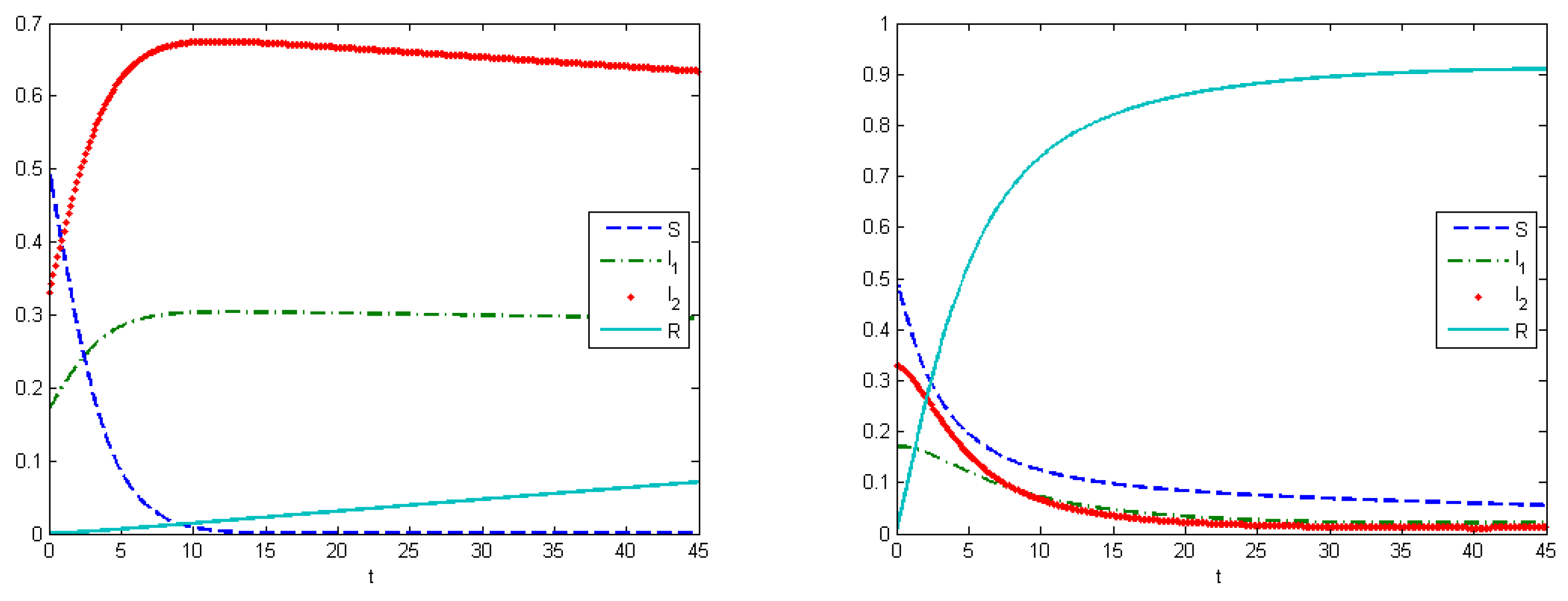
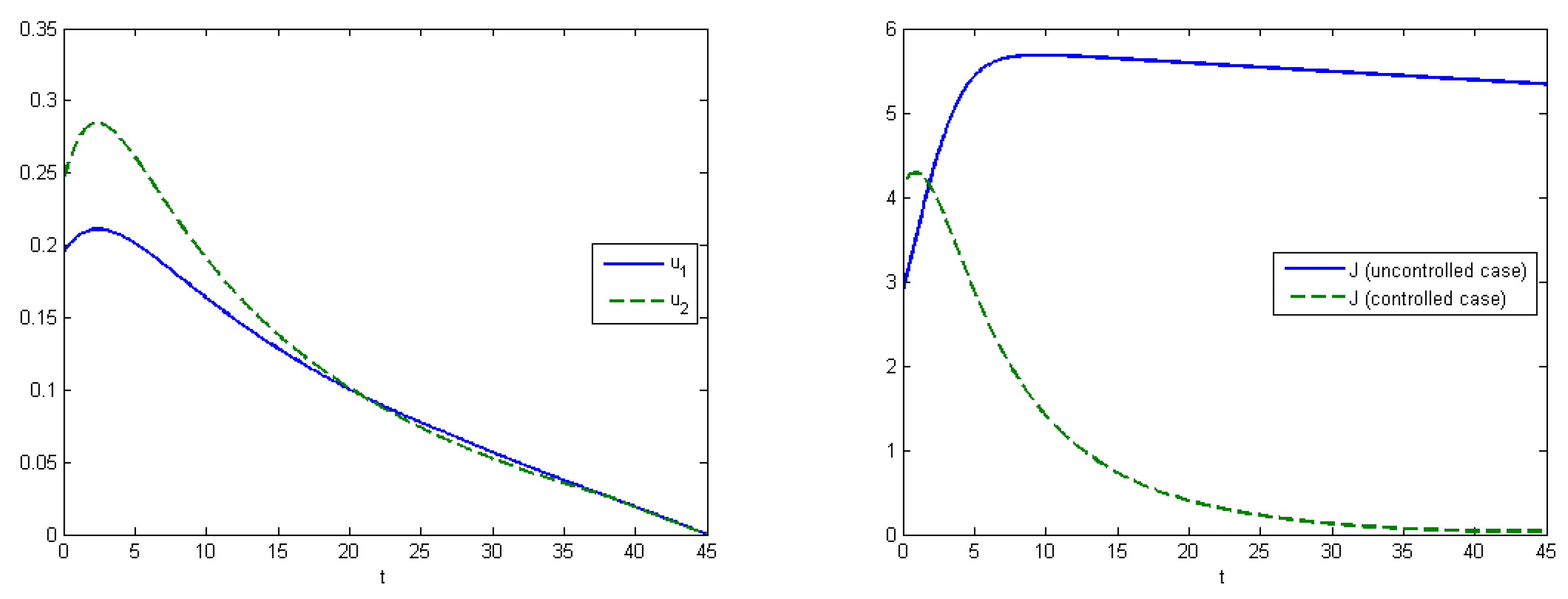
The first experiment shows the behavior of the system in the absence of treatment (control). As a control strategy, we used the medical treatment of the infected host, and the convex form of cost functions, i.e., $h_1\left(u_1\right)=15u_1^2$ and $h_2\left(u_2\right)=10u_2^2$. After simulations, we obtained that the maximum amount of replicas in the case without applying treatment were $I_1\left(t_1\right)=0.3031$ at $t_1=11.25$, and $I_2\left(t_2\right)=0.6742$ at $t_2=10.25$ (Figure 2). From Experiment 1, we can see that, in the absence of treatment in the end of epidemic period, our population had the following distribution of Infected hosts: $29\%$ are infected by first type of virus and $64\%$ are infected by the second type of virus. As we have self-recovery rate ${\sigma }_1=0.001$ and ${\sigma }_2=0.002$, a fraction of the Recovered is $R\left(T\right)=0.07$. In the case when we applied the control, the fraction of infected hosts was zero at the end of interval $T=45$, and the fraction of the recovered was $92\%$. There were also some susceptible nodes ($S\left(T\right)=0.07$) that were not affected by the epidemic. Comparing the controlled and uncontrolled case, the aggregated system costs were: $J=1004.43$ in the uncontrolled model and $J=268.35$ in the controlled model (Figure 3).

Experiment 2 represents the SIR model with virus mutation. Infection rates ${\delta }_i\left(t\right),i=1,2$ indicate the speed of viruses spreading in the population. In our work, it means that we take the competition between viruses for the host into account. Here, we supposed that the stronger virus captures more hosts. The strength of the virus depends on the infection rates, which change under a mutation process. In this experiment, infection rates changed by the formula ${\delta }_i\left(t\right)={\delta }_i(t-\mathsf{\Delta }t)+{\delta }_i(t-\mathsf{\Delta }t)(I_i\left(t\right)-I_i(t-\mathsf{\Delta }t))$ for $i=\{1,2\}$. Evolutionary dynamics allow us to estimate how viruses evolve in an urban population, and to calculate the Nash equilibrium. The Nash equilibrium shows the expected proportions of infected populations after a certain amount of time. This estimation can be useful when building forecasts and tactics to prevent an epidemic. We can allocate available resources in such way that the aggregated costs of the system are minimized. Using the SIR model, we illustrate how the system develops under various types of control.

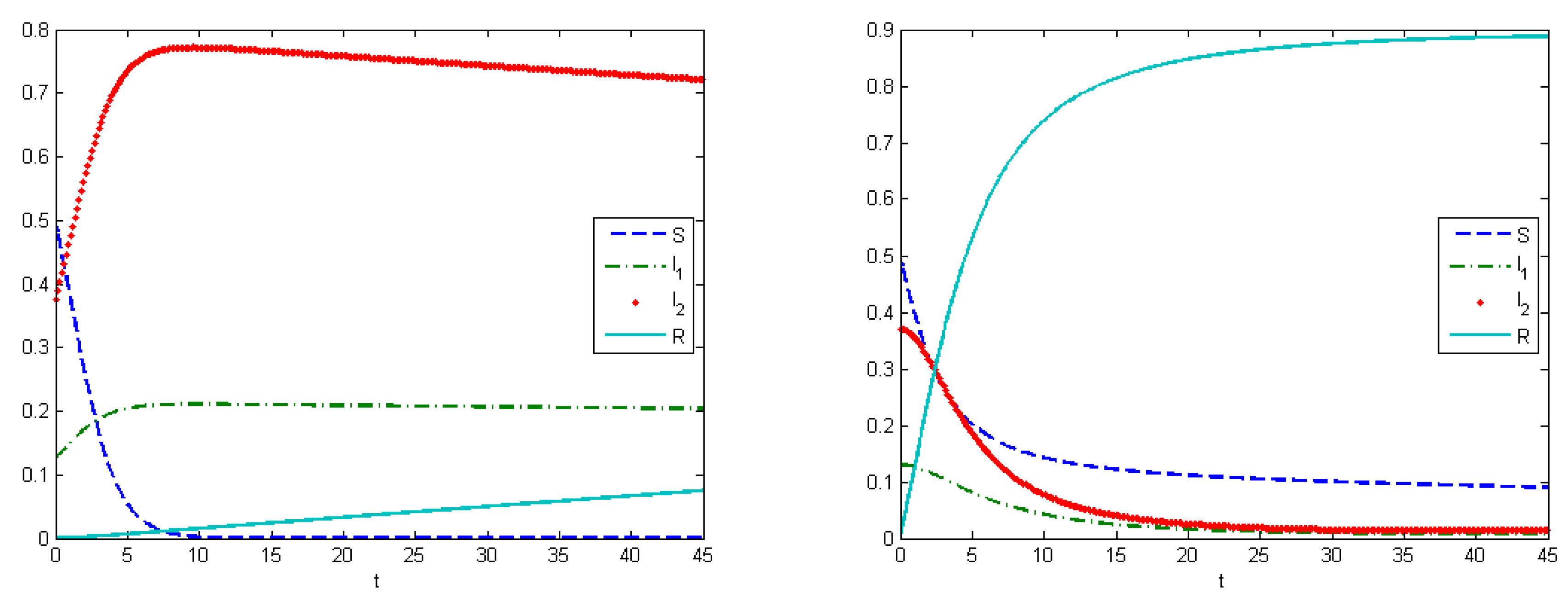
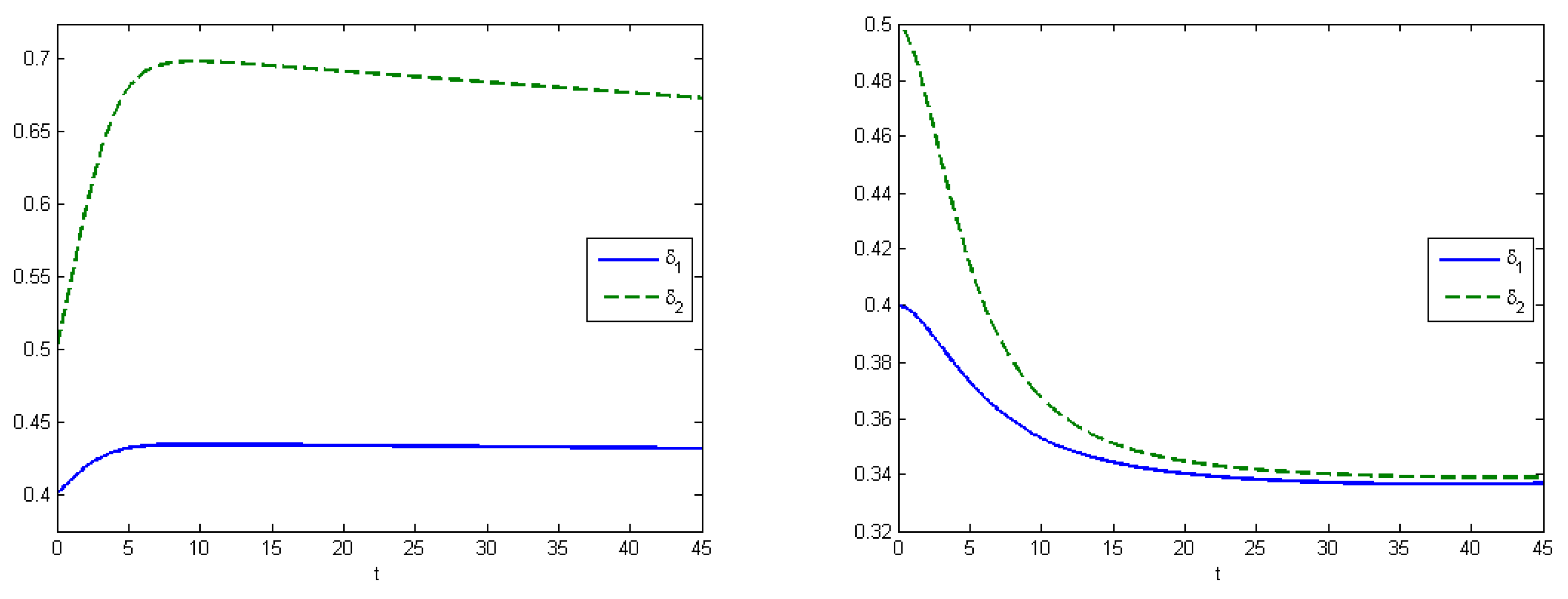
Here, we have utility of occupation functions as $b_1\left(I_1\right)=I_1$ and $b_2\left(I_2\right)=I_2$, and energy-cost functions are $C_1\left(I_1\right)=5I_1$ and $C_2\left(I_2\right)=2I_2$. According to these data, we observed that the Nash equilibrium was equal to $(0.24;0.76)$ in the case when we did not apply any treatment. Figure 4 (left) shows the behavior of the system in the uncontrolled case, where the maximum population of $V_1$ was $I_1\left(t_1\right)=0.2165$ at $t_1=11.25$ and the maximum population of $V_2$ was $I_2\left(t_2\right)=0.7746$ at $t_2=8.5$. By applying optimal treatment strategies, we observed that the maximal values for both types of viruses were equal to their initial state ($I_1\left(0\right)=0.12$ and $I_2\left(0\right)=0.38$). The structure of the optimal control in the case with the virus mutation is shown in Figure 5 (left). Comparison of aggregated costs is presented on Figure 5 (right). The aggregated system cost was $J=1048.5$ in the uncontrolled model and $J=294.59$ in the controlled model.

Experiment 3 shows the SIR model with the virus mutation (Figure 6). Utility-of-occupation functions were $b_1\left(I_1\right)=2I_1$ and $b_2\left(I_2\right)=2I_2$, and energy-cost functions were $C_1\left(I_1\right)=5I_1$ and $C_2\left(I_2\right)=3I_2$. The expected proportions of infected subpopulations were equal to the Nash equilibrium $(0.17;0.83)$, according to simulations we received that the difference between parameters $b_i$ and $C_i$ influences the equilibrium state. From Equation (1), we have that the fraction of the stronger virus is higher if the difference is smaller. Figure 7 demonstrates the change of the infection rates of Experiments 2 and 3. Under the application of optimal control, we have that the maximum values for both types of viruses are equal to their initial state ($I_1\left(0\right)=0.2$ and $I_2\left(0\right)=0.3$).

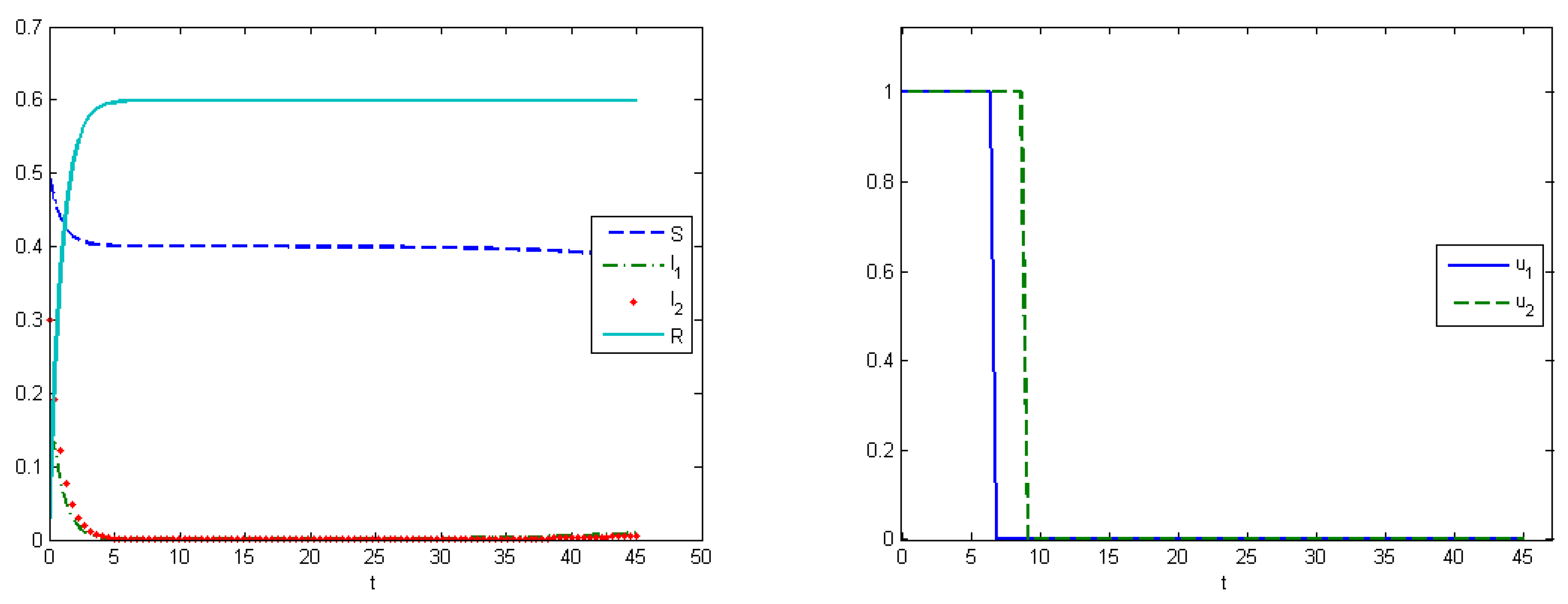
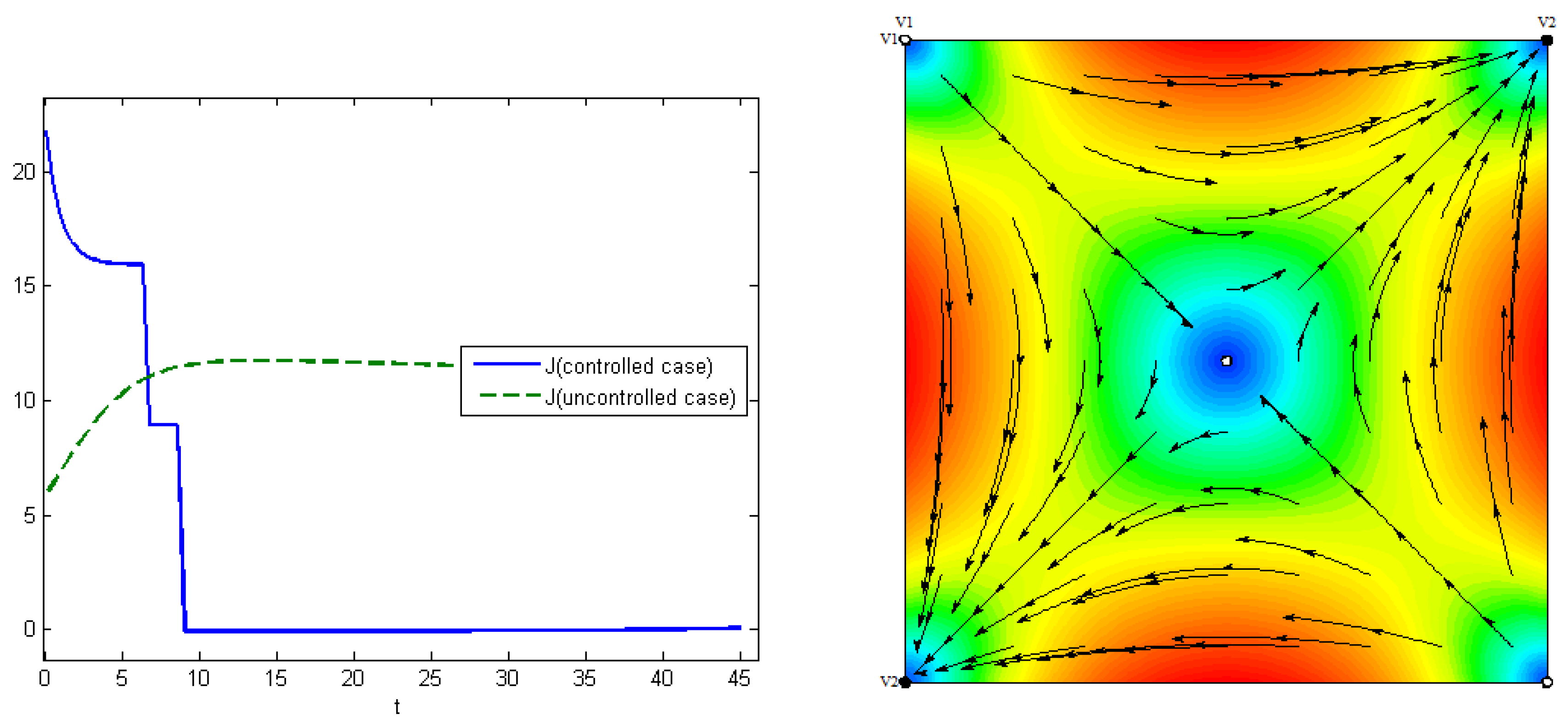
The fourth experiment describes the case when the costs for medical treatments are concave functions. In this case, we have proven in Section 5 that the optimal control has a “bang-bang” structure, i.e., Figure 8 (right). The control for the first type of virus is turned off on the seventh day, and, for the second type, on the ninth day. At the end of interval $T=45$, the proportion of the recovered hosts was $60\%$, while the remaining population was still susceptible to infection. The comparisons of the aggregated costs are presented on Figure 9 (left). Aggregated system cost was $J=1035.4$ in the uncontrolled model and $J=289.42$ in the controlled model.

Figure 9 (right) demonstrates the evolution of viruses over time in human populations. Here, we can see that there are three stationary states corresponding to three Nash equilibria, and that the convergence of solution trajectories of ODE (1) depends on the initial states.

7. Conclusions and Discussion

In this paper, we studied an epidemic model that takes into account the evolutionary dynamics of virus mutations. Different from other studies, we did not consider a group of latent individuals who are already infected but they do not have any clinical symptoms. Many studies have shown that this subgroup can intensively influence epidemic dynamics, but, in the current study, we concentrated on the extended SIR model, including the virus-mutation process. However, we believe that this additional group could enrich our future research. Classical SIR epidemic dynamics are strongly coupled with the replicator dynamics of the virus. We formulated an optimal-control problem in which we sought to minimize the costs of preventing outbreaks by describing the structure of the optimal treatment and quarantine strategies against infection from two different types of viruses. Using Pontryagin’s maximum principle, we showed that, depending on the structure of the cost functions, optimal control has a threshold structure. We corroborated our results with numerical examples, observing different switching times for the control strategies under models with and without virus mutations. As future work, we would extend this study to multiple types of viruses and apply different evolutionary dynamics to model the process of virus mutations, including imitative dynamics and best-response dynamics.

References

- Capasso, V. Mathematical Structures of Epidemic Systems; Lecture Notes in Biomathematics; Springer: Berlin/Heidelberg, Germany, 1993; Volume 97. [Google Scholar]
- Conn, M. Handbook of Models for Human Aging; Academic Press: London, UK, 2006. [Google Scholar]
- Newman, M.E.J. Threshold effects for two pathogens spreading on a network. Phys. Rev. Lett. 2005, 95, 108701. [Google Scholar] [CrossRef] [PubMed]
- Pastor-Satorras, R.; Castellano, C.; Van Mieghem, P.; Vespignani, A. Epidemic processes in complex networks. Rev. Mod. Phys. 2015, 87, 925–979. [Google Scholar] [CrossRef] [Green Version]
- Rota Bulò, S.; Bomze, I. Infection and immunization: A new class of evolutionary game dynamics. Games Econ. Behav. 2011, 71, 193–211. [Google Scholar] [CrossRef] [Green Version]
- Kermack, W.O.; McKendrick, A.G. A contribution to the mathematical theory of epidemics. Proc. R. Soc. 1927, 115, 700–721. [Google Scholar] [CrossRef]
- Wickwire, K.H. A note on the optimal control of carrier-borne epidemics. J. Appl. Probab. 1975, 12, 565–568. [Google Scholar] [CrossRef]
- Behncke, H. Optimal control of deterministic epidemics. Optim. Control Appl. Methods 2000, 21, 269–285. [Google Scholar] [CrossRef]
- Francis, P.J. Optimal tax/subsidy combinations for the flu season. J. Econ. Dyn. Control 2004, 28, 2037–2054. [Google Scholar] [CrossRef]
- Butler, D. Flu surveillance lacking. Nature 2012, 483, 520–522. [Google Scholar] [CrossRef] [PubMed] [Green Version]
- Taynitskiy, V.; Gubar, E.; Zhu, Q. Optimal Security Policy for Protection Against Heterogeneous Malware. In Proceedings of the International Conference on “Network Games, Control and Optimization” (NETGCOOP 2016), Avignon, France, 23–25 November 2016; pp. 199–210. [Google Scholar]
- Khouzani, M.H.R.; Sarkar, S.; Altman, E. Optimal control of epidemic evolution. In Proceedings of the 30th International Conference on Computer Communications (INFOCOM), Shanghai, China, 10–25 April 2011; pp. 1683–1691. [Google Scholar]
- Newman, L.H. What we know about Friday’s massive east coast Internet outage. Wired Magazine, 20 October 2016. [Google Scholar]
- Rohloff, K.R.; Başar, T. Deterministic and stochastic models for the detection of random constant scanning worms. ACM Trans. Model. Comput. Simul. (ACM TOMACS) 2008, 18, 1–24. [Google Scholar] [CrossRef]
- Khouzani, M.H.R.; Sarkar, S.; Altman, E. Dispatch then stop: Optimal dissemination of security patches in mobile wireless networks. In Proceedings of the 48th IEEE Conference on Decisions and Control (CDC), Atlanta, Georgia, USA, 15–17 December 2010; pp. 2354–2359. [Google Scholar]
- Khouzani, M.H.R.; Sarkar, S.; Altman, E. Maximum damage malware attack mobile wireless networks. In Proceedings of the 29th International Conference on Computer Communications (INFOCOM), San Diego, CA, USA, 15–19 March 2010; pp. 749–757. [Google Scholar]
- Omic, J.; Orda, A.; Van Mieghem, P. Protecting against network infections: A game theoretic perspective. In Proceedings of the 28th IEEE Conference on Computer Communications (INFOCOM), Rio de Janeiro, Brazil, 19–25 April 2009. [Google Scholar]
- Zhu, Q.; Bushnell, L.; Başar, T. Game-theoretic analysis of node capture and cloning attack with multiple attackers in wireless sensor networks. In Proceedings of the 51st IEEE Conference on Decision and Control (CDC’12), Maui, HI, USA, 10–13 December 2012. [Google Scholar]
- Fu, F.; Rosenbloom, D.; Wang, L.; Nowak, M. Imitation dynamics of vaccination behaviour on social networks. Proc. R. Soc. Lond. Ser. B 2011, 278, 42–49. [Google Scholar] [CrossRef] [PubMed] [Green Version]
- Taynitskiy, V.A.; Gubar, E.A.; Zhitkova, E.M. Structure of optimal control in the model of propagation of two malicious softwares. In Proceedings of the International Conference “Stability and Control Processes” in Memory of V.I. Zubov (SCP), Saint-Petersburg, Russia, 5–9 October 2015; pp. 261–264. [Google Scholar]
- Chowell, G.; Viboud, C.; Merler, S.; Vespignani, A. Perspectives on model forecasts of the 2014–2015 Ebola epidemic in West Africa: Lessons and the way forward. BMC Med. 2017, 15, 42. [Google Scholar] [CrossRef] [PubMed]
- Gjorgjieva, J.; Smith, K.; Chowell, G.; Sanchez, F.; Snyder, J.; Castillo-Chavez, C. The role of vaccination in the control of SARS. Math. Biosci. Eng. 2005, 2, 753–769. [Google Scholar] [PubMed]
- Bonhoeffer, S.; May, R.M.; Shaw, G.M.; Nowak, M.A. Virus dynamics and drug therapy. Proc. Natl. Acad. Sci. USA 1997, 94, 6971–6976. [Google Scholar] [CrossRef] [PubMed] [Green Version]
- Gubar, E.; Zhu, Q. Optimal Control of Influenza Epidemic Model with Virus Mutations. In Proceedings of the 12th Biannual European Control Conference, Zurich, Switzerland, 17–19 July 2013; IEEE Control Systems Society: New York, NY, USA, 2013; pp. 3125–3130. [Google Scholar]
- Maynard, S.J. Evolution and the Theory of Games; Cambridge University Press: Cambridge, UK, 1982. [Google Scholar]
- Weibull, J. Evolutionary Game Theory; The M.I.T. Press: Cambridge, MA, USA, 1995. [Google Scholar]
- Taylor, P.D.; Jonker, L.B. Evolutionarily stable strategies and game dynamics. Math. Biosci. 1978, 40, 145–156. [Google Scholar] [CrossRef]
- Khatri, S.; Rael, R.; Hyman, J. The Role of Network Topology on the Initial Growth Rate of Influenza Epidemic; Technical Report BU-1643-M; KeAi: Beijing, China, 2003. [Google Scholar]
- Pontryagin, L.S.; Boltyanskii, V.G.; Gamkrelidze, R.V.; Mishchenko, E.F. The Mathematical Theory of Optimal Processes; Interscience Publishers: Hoboken, NJ, USA, 1962. [Google Scholar]
Figure 1.
Transition rule: Scheme describes the reaction to two heterogeneous viruses circulating in a population. We assumed that the epidemic process could be controlled using treatment or quarantine methods. These measures can be considered as the control parameters in the system, which are used to reduce the size of the infected population and terminate the epidemic process.
Figure 2.
Experiment 1. Left: SIR model without virus mutation and without applying control. Initial states are , , maximum values are and . Epidemic peaks a reached at 11th and 10th days. Right: SIR model without virus mutation with application of control. Vertical axes show the fractions of the subpopulations.
Figure 3.
Experiment 1. Left: Optimal control in SIR model without virus mutation; cost functions are convex . Vertical axis shows the amount of applied control. Right: Comparison of aggregated costs of SIR model without virus mutation (Controlled model: ; uncontrolled model: ). Vertical axis shows the aggregated costs at time moment t in m.u.
Figure 4.
Experiment 2. Left: SIR model with virus mutation and without applying control. Maximum values are , . Epidemic peaks reached at the 11th and 8th days. Right: SIR model with virus mutation and application of control. Functions were convex. Vertical axes show the fractions of the subpopulations.
Figure 5.
Experiment 2. Left: Optimal control in the SIR model with virus mutation and convex cost functions . Vertical axis shows the amount of applied control. Right: Comparison of aggregated costs of the SIR model with virus mutation (Controlled model , uncontrolled model ). Vertical axis shows the aggregated costs at time moment t in m.u.
Figure 6.
Experiment 3. Left: SIR model with virus mutation and application of control. Functions are convex. Vertical axis shows the fractions of the subpopulations. Right: Optimal control in SIR model with virus mutation and convex-cost functions . Vertical axis shows the amount of applied control at time moment t.
Figure 7.
Left: Experiment 2. Infected rates of the SIR model with virus mutations (uncontrolled case). Utility-of-occupation functions were and . Cost functions were and . Infectious rates were and . Right: Experiment 3. Infected rates of the SIR model with virus mutations (controlled case). Utility-of-occupation functions were and . Cost functions were and . Infectious rates were and .
Figure 8.
Experiment 4. Left: SIR model with virus mutation and application of control. Functions are concave. Vertical axis shows the fractions of the subpopulations. Right: Optimal control in SIR model with virus mutation and concave-cost functions . Control was switched off at the seventh day for , and at the ninth day for . Vertical axis shows the amount of applied control at time moment t.
Figure 9.
Left: Experiment 4. Comparison of aggregated costs of the SIR model with virus mutation (Controlled model , uncontrolled model ). Vertical axis shows the aggregated costs at time moment t in m.u. Right: Simplex of mixed strategies of the symmetric bimatrix game for modeling virus mutations. In this numerical example, the set of Nash equilibrium was found to be .
© 2018 by the authors. Licensee MDPI, Basel, Switzerland. This article is an open access article distributed under the terms and conditions of the Creative Commons Attribution (CC BY) license (http://creativecommons.org/licenses/by/4.0/).
Share and Cite
MDPI and ACS Style
Gubar, E.; Taynitskiy, V.; Zhu, Q. Optimal Control of Heterogeneous Mutating Viruses. Games 2018, 9, 103. https://doi.org/10.3390/g9040103
AMA Style
Gubar E, Taynitskiy V, Zhu Q. Optimal Control of Heterogeneous Mutating Viruses. Games. 2018; 9(4):103. https://doi.org/10.3390/g9040103
Chicago/Turabian StyleGubar, Elena, Vladislav Taynitskiy, and Quanyan Zhu. 2018. "Optimal Control of Heterogeneous Mutating Viruses" Games 9, no. 4: 103. https://doi.org/10.3390/g9040103
Note that from the first issue of 2016, this journal uses article numbers instead of page numbers. See further details here.