On the Phase Diagrams of ⁴He Adsorbed on Graphene and Graphite from Quantum Simulation Methods

Abstract

The ground-state phase diagrams of ${}^4$He adsorbed on graphene and graphite are calculated using quantum simulation methods. In this work, a systematic investigation of the approximations used in such simulations is carried out. Particular focus is placed on the helium–helium (He–He) and helium–carbon (He–C) interactions, as well as their modern approximations. On careful consideration of other approximations and convergence, the simulations are otherwise (numerically) exact. The He–He interaction as approximated by a sum of pairwise potentials is quantitatively assessed. A similar analysis is made for the He–C interaction, but more thoroughly and with a focus on surface corrugation. The importance of many-body effects is discussed. Altogether, the results provide “reference data” for the considered systems. Using comparisons with experiments and first-principle calculations, conclusions are drawn regarding the quantitative accuracy of these modern approximations to these interactions.

1. Introduction

Quantum fluids and solids (QFS) are characterized by particles that interact through weak long-range forces, and for which their quantum kinetic energy $E_{\mathrm{k}}$ is much larger than $k_{\mathrm{B}}T$ where $k_{\mathrm{B}}$ is the Boltzmann constant and T is the temperature. For the solid phase [1], the quantum motion can lead to spatial fluctuations about the equilibrium lattice sites that are much larger than in any classical solid. These phases are important for several reasons, as they are key to the fundamental understanding of nature, technological applications, and applied interests of many scientific fields.

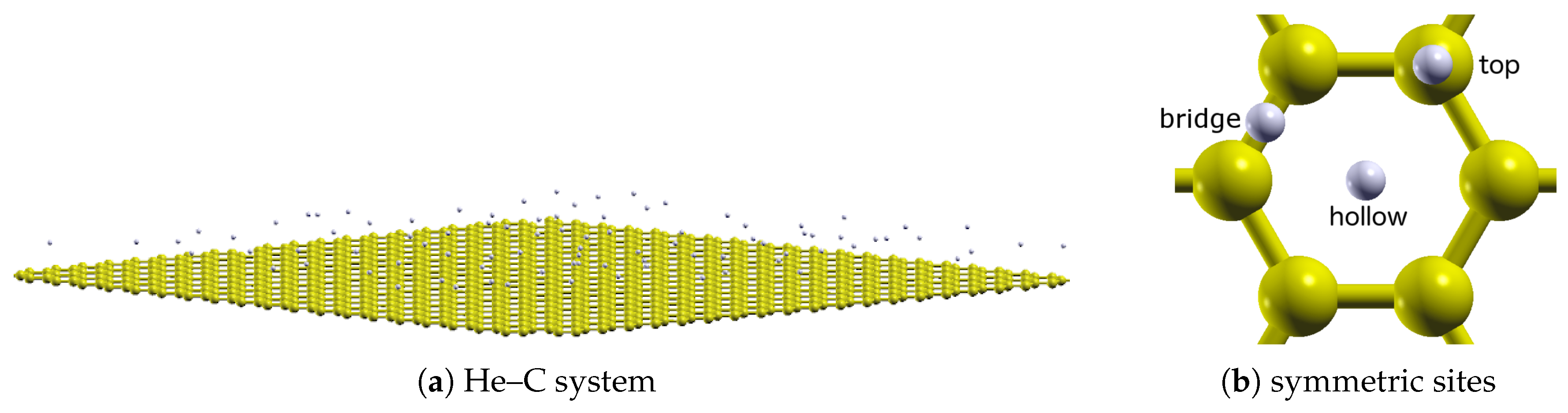
QFS often consist of lightweight particles (because of their large $E_{\mathrm{k}}$). Archetypical examples include hydrogen and helium, which are present in a wide range of thermodynamic conditions [2]. One such system that is the subject of many experimental and theoretical studies is the adsorption of helium on a carbon (often graphene or graphite) substrate. An example of this system is shown in Figure 1.

While studies of this system have been performed over several decades now, it is currently of interest with respect to its possible connection to a supersolid phase of matter [3].

Due to the strong attraction to the substrate, helium atoms adsorb layer by layer through at least seven distinct ones on graphite [4]. For the first two, equivalent densities are respectively about $1.5$ and $1.1$ times that of the bulk liquid, and highly compressed in vertical separation from the surface. In addition, several phases result from the interaction between the helium atoms (which will be referred to as the He–He interaction) and their interaction with the substrate (the He–C interaction). These have been studied computationally for both graphene [5,6,7,8,9,10] and graphite [5,6,11,12,13,14,15]. Experimental references will be made within this context.

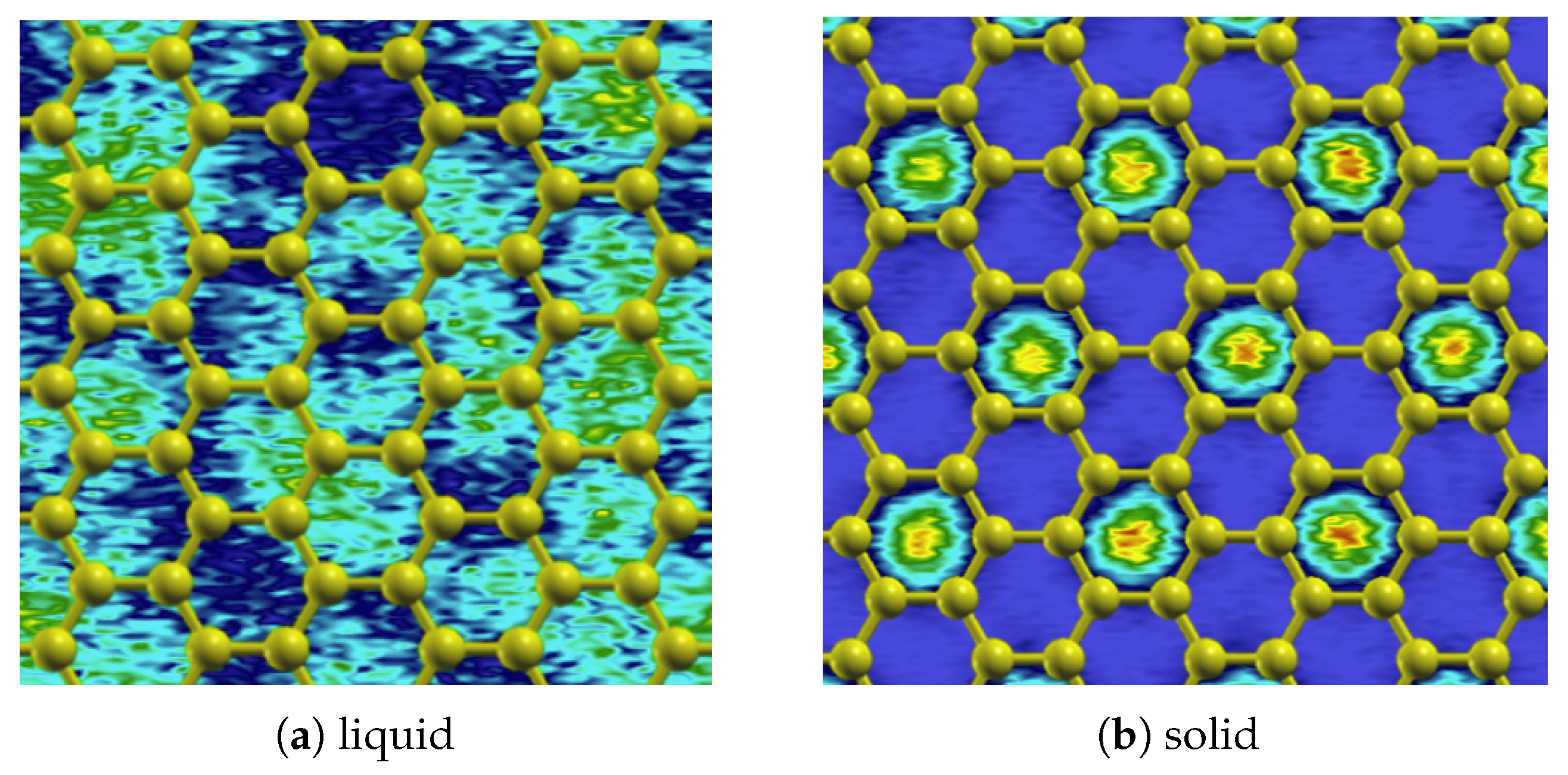
For the first adsorbed helium layer, the phase diagram is only somewhat understood. It is well established from heat-capacity [16,17] and neutron-diffraction [18] measurements that a commensurate (C) solid phase is stable in which one-third ($1/3$) of the available substrate adsorption sites (the hollow sites; see Figure 1b) are occupied in a $\sqrt{3}\times \sqrt{3}$ structure (called the $C_{1/3}$ phase); a representative density plot of this phase is shown in Figure 2b. At lower densities, it has been suggested (from experiments [19]) that the solid melts, forming a low-temperature liquid (possibly a superfluid) phase; an alternative scenario (from calculations [13]) is that the low-density monolayer is comprised of solid clusters and a low-density vapor.

While the general structural features in this region of the phase diagram seem somewhat established, the properties are less so and controversial. Consider again a possible supersolid phase (supersolidity is not actually considered herein, but the idea is nonetheless a motivation). For the first adsorbed layer, this was calculated in [6]. Additional calculations [7], however, suggested that the superfluidity and structural properties for the related vacancies could be a feature of the assumed He–C interaction. (The possibility of supersolidity has also been suggested for the second adsorbed layer [20]; for an opposing view, see [15].)

In this article, a relatively fundamental question is considered based on these results: Are the approximations to the interactions used in quantum simulations capable of achieving quantitative accuracy, even for the phase diagram? This is answered for the adsorption of ${}^4$He to graphene and graphite substrates. The quantitative accuracy of modern approximations to the He–He and He–C interactions are systematically investigated. These include the recently-proposed He–He pairwise potential of Przybytek et al. [21,22] and the He–C atom–bond pairwise potential [23] (both are discussed and motivated further in Section 2). Careful consideration of other approximations and convergence are made as well. Related questions are also considered: Are the He–C interactions developed for graphite suitable for studying graphene, and vice versa? In terms of interactions, why does graphite have a similar phase diagram to graphene? Etc.

This article is outlined as follows. The quantum simulation methods used are discussed next (Section 2). Results are then presented (Section 3). Following this, they are discussed (Section 4). Finally, conclusions are drawn and an outlook is provided (Section 5).

2. Methods

The ground-state phase diagrams of ${}^4$He adsorbed on graphene and graphite were calculated using quantum simulation methods. The ${}^4$He atoms were modeled quantum mechanically, under the adiabatic (approximation to the) elimination of the electronic degrees of freedom [24] (a priori, there is no reason to expect this approximation to be invalid). The carbon atoms, on the other hand, were modeled as classical, fixed particles.

The solution to the above problem is that of the many-body Schrödinger equation $\Psi (\mathbf{r};\mathbf{R})$ where $\mathbf{r}$ represents the ${}^4$He coordinates, parameterized on the carbon ones $\mathbf{R}$,

$$\mathcal{H}\Psi (\mathbf{r};\mathbf{R})=E\Psi (\mathbf{r};\mathbf{R})$$

(1)

where the Hamiltonian $\mathcal{H}$ describing the system under the above approximations is

$$\mathcal{H}=\sum _{i=1}^{N_{{}^4\mathrm{He}}}\frac{{-\hslash }^2}{{{2m}_4}_{\mathrm{He}}}{\nabla }_i^2+{\mathcal{V}}_{\mathrm{He}\text{–}\mathrm{He}}+{\mathcal{V}}_{\mathrm{He}\text{–}\mathrm{C}}$$

(2)

where the first term sums over the number of ${}^4$He atoms $N_{{}^4\mathrm{He}}$, ${\mathcal{V}}_{\mathrm{He}\text{–}\mathrm{He}}$ and ${\mathcal{V}}_{\mathrm{He}\text{–}\mathrm{C}}$ are the He–He and He–C interactions, respectively, and E is the energy.

The He–He interaction was modeled as a sum of pairwise potentials,

$${\mathcal{V}}_{\mathrm{He}\text{–}\mathrm{He}}\left(\mathbf{r}\right)=\sum _{(i,j)}^{{N_4}_{\mathrm{He}}}{V}_{\mathrm{He}\text{–}\mathrm{He}}\left(r_{ij}\right)$$

(3)

where $V_{\mathrm{He}\text{–}\mathrm{He}}$$\left(r_{ij}\right)$ is the potential between ${}^4$He atoms separated by a distance $r_{ij}=|{\mathbf{r}}_i-{\mathbf{r}}_j|$, and the sum runs over all such pairs $(i,j)$. Forms of $V_{\mathrm{He}\text{–}\mathrm{He}}$ considered were the HFD-B form [25] with the parameters of Aziz for helium from [26] and the more modern pairwise form of Przybytek et al. [21,22,27]. Note that the latter leads to better agreement with the experimental phase diagram of bulk ${}^4$He at all densities. For a recent evaluation of He–He potentials for predicting the ground-state energies and structural properties of the helium dimer (and trimers), see [28].

The He–C interaction was modeled as a sum of potentials between each ${}^4$He atom and the substrate,

$${\mathcal{V}}_{\mathrm{He}\text{–}\mathrm{C}}(\mathbf{r};\mathbf{R})=\sum _{i=1}^{{N_4}_{\mathrm{He}}}{V}_{\mathrm{He}\text{–}\mathrm{C}}({\mathbf{r}}_i;\mathbf{R})$$

(4)

where $V_{\mathrm{He}\text{–}\mathrm{C}}({\mathbf{r}}_i;\mathbf{R})$ is the potential between atom i and the entire carbon lattice (described by $\mathbf{R}$). Forms of $V_{\mathrm{He}\text{–}\mathrm{C}}$ considered were the 6–12 isotropic and anisotropic potentials [29] (both which can be written as a sum of pairwise potentials between helium and carbon atoms) and a more modern atom–bond pairwise potential [23] (which considers the interaction as additive atom–bond pairwise potentials [30] between helium atoms and carbon–carbon bonds [31]). Note that these potentials are based on different (types of) data; the former are the best fits to that from scattering experiments (for graphite), whereas the latter is fitted to that from first-principles calculations (for a model system for graphene). Because these forms of the He–C interaction are (all) decomposed as a sum of pairwise potentials, they can straightforwardly be (and are commonly) applied to different substrates (graphene or graphite, respectively). Though, it is an approximation that this can be done with equal accuracy.

Quantum Monte Carlo methods [32] were used to stochastically solve Equation (1). Both variational (VMC) and diffusion Monte Carlo (DMC) were used, as described below.

VMC was used first to variationally find the optimal parameters of a trial (T) solution ${\Psi }_{\mathrm{T}}$ to Equation (1). That considered was a symmetrized version [33] (and, in particular, its extension to two dimensions [34]) of the Nosanow–Jastrow form,

$${\Psi }_{\mathrm{T}}(\mathbf{r};\mathbf{R})=\left\{\prod _{(i,j)}^{{N_4}_{\mathrm{He}}}f\left(r_{ij}\right)\right\}\left\{\prod _{J=1}^{N_{\mathrm{s}}}\left(\sum _{i=1}^{{N_4}_{\mathrm{He}}}g\left(r_{iJ}^{xy}\right)\right)\right\}\left\{\prod _{i=1}^{{N_4}_{\mathrm{He}}}\psi \left(z_i\right)\right\}$$

(5)

where

$$f\left(r_{ij}\right)=e^{-\frac{1}{2}{\left(\frac{b_{\mathrm{He}\text{–}\mathrm{He}}}{r_{ij}}\right)}^5}$$

is a two-body (atoms i and j) correlation function,

$$g\left(r_{iJ}^{xy}\right)=e^{-{\alpha }_{\mathrm{He}\text{–}\mathrm{C}}{r_{iJ}^{xy}}^2}$$

is a one-body localization factor, which localizes atom i to the sites $J=1,2,\dots ,N_{\mathrm{s}}$ where $N_{\mathrm{s}}$ is number of solid (s) sites and $r_{iJ}^{xy}$ is the magnitude of the vector ${\mathbf{r}}_i-{\mathbf{R}}_J$ projected over the $xy$-plane, and $\psi \left(z_i\right)$ is a localization factor along the z direction. Note that this wavefunction properly and simultaneously accounts for the Bose–Einstein statistics of ${}^4$He, the necessary requirements of spatial solid order, and localization of particles along z.

$\psi$ was numerically calculated using a Numerov integration scheme [35], and according to the approach discussed in Section 3.2. The variational parameters of ${\Psi }_{\mathrm{T}}$ (Equation (5)) are $b_{\mathrm{He}\text{–}\mathrm{He}}$ and ${\alpha }_{\mathrm{He}\text{–}\mathrm{C}}$. The former was determined first and for the liquid phase (i.e., for ${\alpha }_{\mathrm{He}\text{–}\mathrm{C}}=0$), at the equilibrium density; the optimal value found was $3.04$ Å. Keeping this value fixed, ${\alpha }_{\mathrm{He}\text{–}\mathrm{C}}$ was determined for the solid ($C_{1/3}$) phase; the value found was $0.43$ Å${}^{-2}$.

Following this, DMC was used to project out the ground-state solution $\Psi$ (Equation (1)). Note that in this case of bosonic particles, the DMC method is (numerically) exact (i.e., to within statistical uncertainties). VMC, on the other hand, only provides a variational upper-bound to the true energy, depending on the trial wavefunction. In DMC, this wavefunction acts only as a “guiding” function; the quality which is related to convergence.

The He–C systems modeled consisted of $21\times 21$ unit cells of graphene (882 carbon atoms, and /layer, in the case of graphite).

Phase Diagrams

Phase diagrams are presented using the data obtained from the DMC simulations. Note that all energies are reported per particle ($/{N_4}_{\mathrm{He}}$). Note also that statistics (error bars) were calculated using blocking.

Liquid (l) energies $E_{\mathrm{l}}$ as a function of (surface) density $\sigma$ were fit to the commonly-used form

$$E_{\mathrm{l}}\left(\sigma \right)=E_{\mathrm{l}}\left({\sigma }_{\mathrm{eq}}\right)+B{\left(\frac{\sigma -{\sigma }_{\mathrm{eq}}}{{\sigma }_{\mathrm{eq}}}\right)}^2+C{\left(\frac{\sigma -{\sigma }_{\mathrm{eq}}}{{\sigma }_{\mathrm{eq}}}\right)}^3$$

(6)

where the equilibrium density is ${\sigma }_{\mathrm{eq}}$, the energy at this density is $E_{\mathrm{l}}\left({\sigma }_{\mathrm{eq}}\right)$, and A and B are constants.

The stability of the solid (including as the ground state) and also any region(s) of phase coexistence (with the liquid) were determined by double-tangent Maxwell constructions.

3. Results

In this section, the importance of the He–He and He–C interactions are first considered. The focus is on the phase diagram of ${}^4$He adsorbed on graphene—in particular, for monolayer coverages up to and just above the density of the $C_{1/3}$ phase at ${\sigma }_{\mathrm{s}}\approx 0.0636$ Å${}^{-2}$. An extension to graphite is then made. These results are sufficient to make both qualitative and quantitative comparisons to available experimental and first-principles data; this though is reserved for Section 4.

Note that, among the following subsections, results are repeated in a few instances. This is only to simplify the comparative analysis, and will be explicitly remarked on when done so.

3.1. He–He Interaction

Consider first the He–He interaction. In this section, this is considered directly; some aspects of this will be (indirectly) considered again in Section 3.2. Note that the following results were all obtained using the isotropic He–C potential to model the associated interaction.

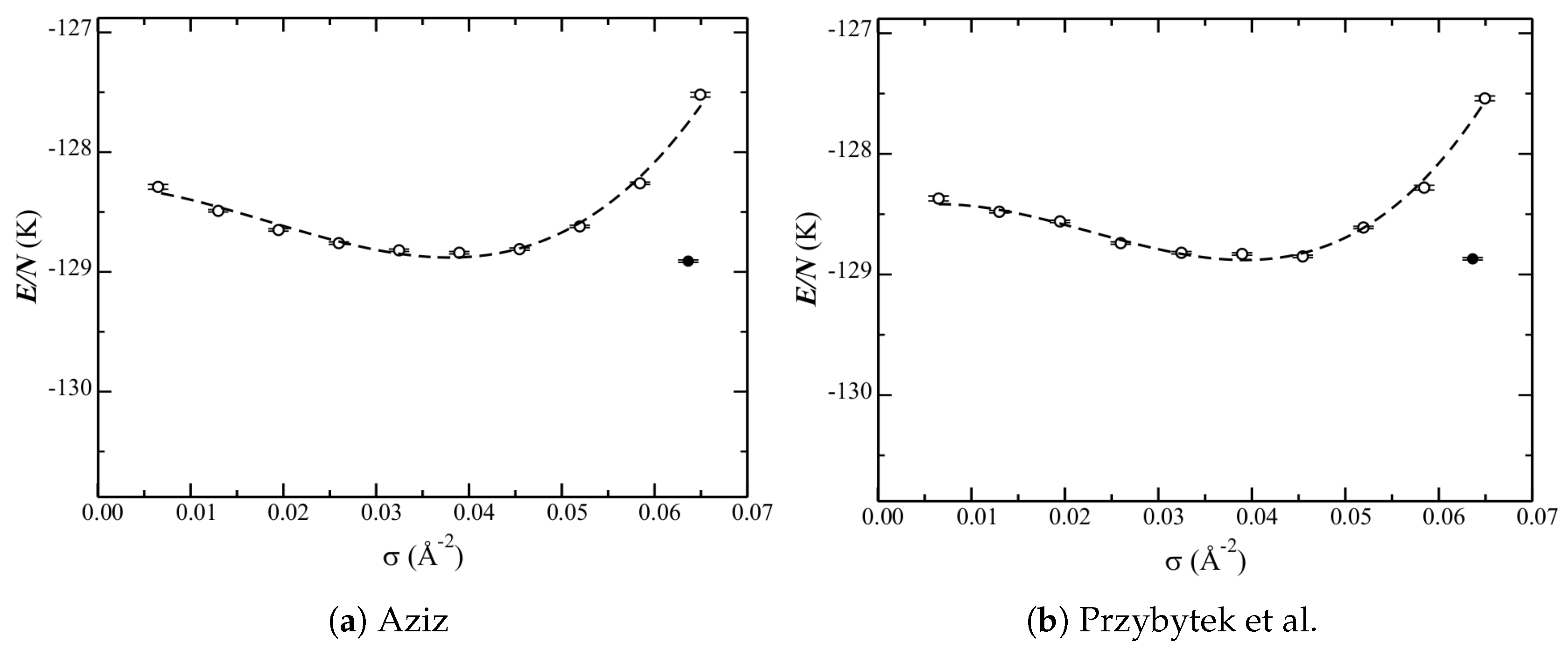
Figure 3 shows the phase diagrams for the two He–He potentials under consideration (Section 2). Corresponding data is reported in

Table 1. The data which corresponds to Figure 3. Results are shown for the two helium–helium (He–He) potentials V${}_{\mathrm{He}-\mathrm{He}}$ under consideration. Note that all quantities have been defined in relation to Equation (6) or at the start of (this) Section 3, except for the energy of the solid $E_{\mathrm{s}}$.

V${}_{\mathbf{He}-\mathbf{He}}$	${\mathit{\sigma }}_{\mathbf{eq}}$ (Å${}^{-2}$)	${\mathit{E}}_{\mathbf{l}}\left({\mathit{\sigma }}_{\mathbf{eq}}\right)$ (K)	${\mathit{E}}_{\mathbf{s}}\left({\mathit{\sigma }}_{\mathbf{s}}\right)$ (K)	${\mathit{E}}_{\mathbf{l}}\left({\mathit{\sigma }}_{\mathbf{s}}\right)$ (K)
Aziz	$0.0379\left(9\right)$	$-128.88\left(2\right)$	$-128.91\left(1\right)$	$-127.8\left(2\right)$
Przybytek et al.	$0.0392\left(6\right)$	$-128.88\left(2\right)$	$-128.87\left(1\right)$	$-127.7\left(1\right)$

. Qualitatively, the two potentials produce nearly identical results. Quantitatively, however, the potential of Przybytek et al. gives an important shift (higher) of the equilibrium liquid density (see below). The energies are otherwise relatively unaffected.

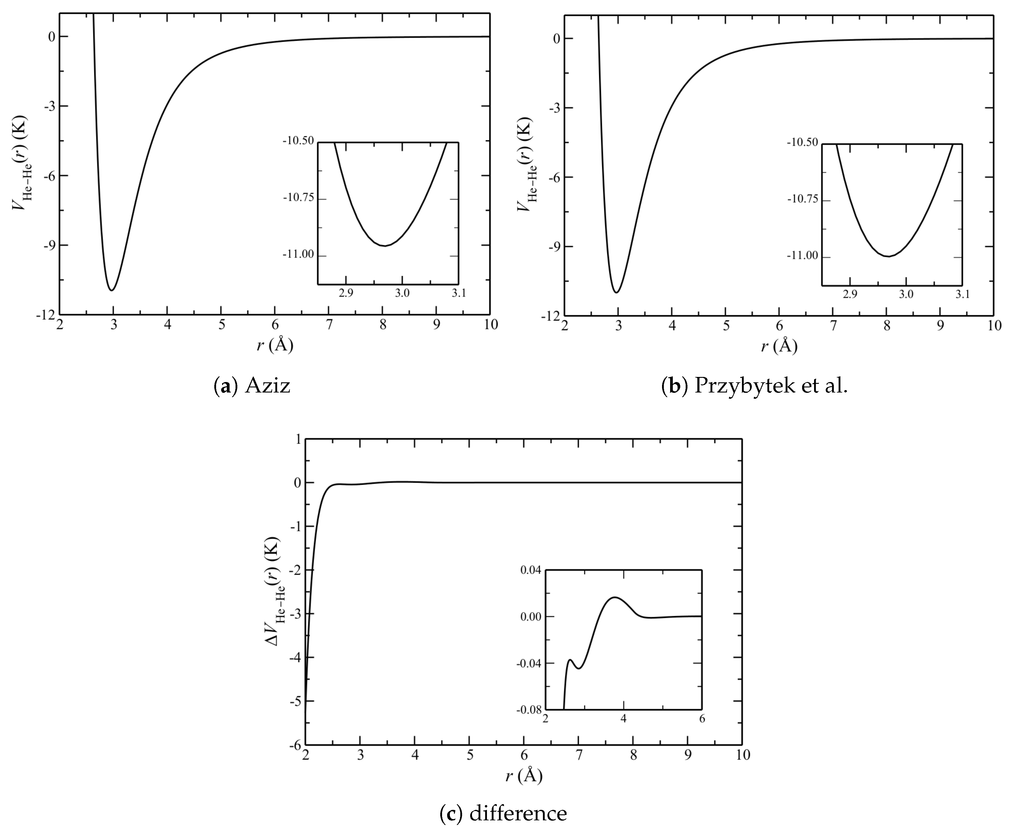
In order to understand the above results, Figure 4 shows the He–He potentials. As expected, they are very similar; this statement refers to both the locations of the minima and the general shapes on either side of them. The improvements of Przybytek et al. result in only a small increase in the well depth.

For the remainder of (this) Section 3, results based only on the He–He potential of Przybytek et al. are shown. In Section 4, it is discussed that this potential leads to an important quantitative improvement in comparison with experiment. Note that the other aspects of the considered systems are probably relatively insensitive to this choice in any case.

3.2. He–C Interaction

Consider now the He–C interaction. While the importance of corrugation has been considered before (either directly (e.g., [14]) or indirectly), thorough quantitative details are considered here.

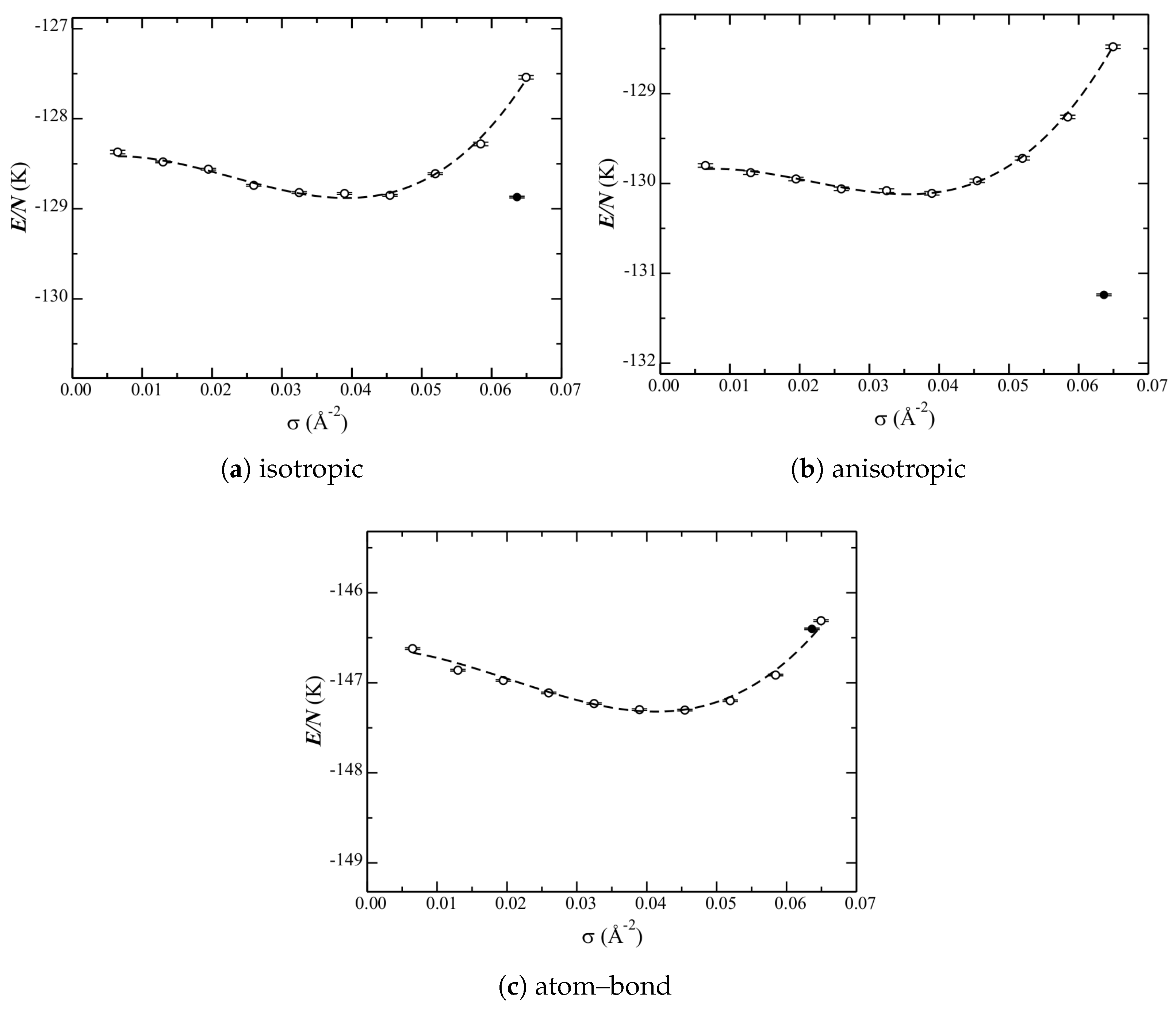
The phase diagram calculated with each of the three He–C potentials under consideration (Section 2) is shown in Figure 5. The corresponding data is reported in

Table 2. Corresponding data to Figure 5. Results are shown for the three helium–carbon (He–C) potentials V${}_{\mathrm{He}-\mathrm{C}}$ under consideration.

V${}_{\mathbf{He}-\mathbf{C}}$	${\mathit{\sigma }}_{\mathbf{eq}}$(Å${}^{-2}$)	${\mathit{E}}_{\mathbf{l}}\left({\mathit{\sigma }}_{\mathbf{eq}}\right)$ (K)	${\mathit{E}}_{\mathbf{s}}\left({\mathit{\sigma }}_{\mathbf{s}}\right)$ (K)	${\mathit{E}}_{\mathbf{l}}\left({\mathit{\sigma }}_{\mathbf{s}}\right)$ (K)
isotropic	$0.0392\left(6\right)$	$-128.88\left(2\right)$	$-128.87\left(1\right)$	$-127.7\left(1\right)$
anisotropic	$0.0355\left(5\right)$	$-130.12\left(1\right)$	$-131.24\left(1\right)$	$-128.6\left(2\right)$
atom–bond	$0.0413\left(7\right)$	$-147.32\left(3\right)$	$-146.401\left(9\right)$	$-146.79\left(9\right)$

.

The liquid curves are qualitatively similar for the isotropic and anisotropic potentials. That of the atom–bond though is different. Quantitatively, each potential has a different relative depth at the minimum (the equilibrium liquid density). From the low-density side, and from shallowest to deepest, are the curves for the anisotropic, isotropic, and atom–bond potentials. On the high-density side, the isotropic and anisotropic curves increase in energy significantly. The atom–bond potential, however, does not. There are also differences in the equilibrium liquid densities among the potentials. The anisotropic one results in the lowest density, whereas that of the atom–bond is just a bit higher than that of the isotropic one. Therefore, while the atom–bond potential looks qualitatively different, this could be related to the higher equilibrium liquid density shifting the entire curve higher.

The (relative) energies of the solid phase are significantly different for the three potentials. For the isotropic one (Figure 5a), the energy of the $C_{1/3}$ structure and the liquid at the equilibrium density are nearly within error bars (Table 2); therefore, the latter is stable (approximately) only at a single point. The anisotropic potential (Figure 5b), however, significantly lowers the energy of the $C_{1/3}$ structure; the solid is unambiguously the ground state. These results are in good agreement with previous calculations [5,6,7,8,9,10], but with using a different He–He potential. The atom–bond potential, however, raises the energy of the $C_{1/3}$ structure above that of the liquid. Note that a probable contribution to this is the shallow increase in energy of the high(er)-density liquid (as discussed above).

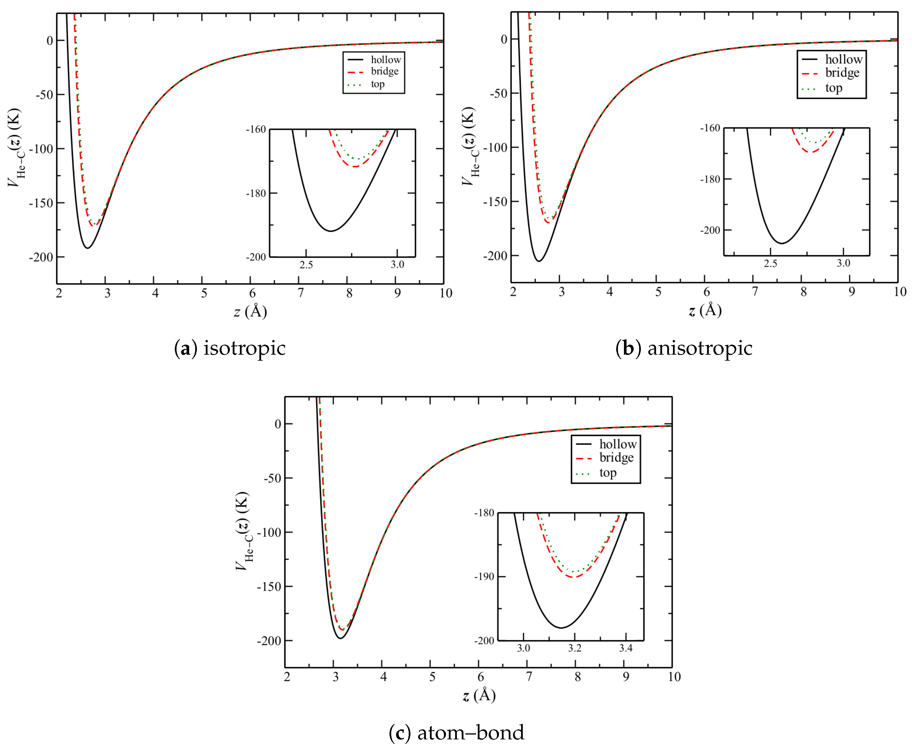
To understand the above, it is necessary to consider the quantitative properties of these potentials. Of particular importance is their corrugation, herein defined to be the relative difference in potential between the high-symmetry sites over the graphene plane (Figure 1b). This can be seen by $V_{\mathrm{He}\text{–}\mathrm{C}}$$\left(z\right)$, the He–C potential for a single helium atom as a function of its height z over the carbon surface.

The potentials $V_{\mathrm{He}\text{–}\mathrm{C}}$$\left(z\right)$ over the sites in Figure 1b for each of the He–C potentials are shown in Figure 6. Qualitatively, they are similar. The well depths increase from top and bridge to the hollow sites for each. In addition, the (relative) well depths for the bridge and top sites are comparable. Quantitatively however, those for the hollow sites are noticeably different. That for the anisotropic potential is largest, whereas that for the atom–bond potential is comparable to the other sites.

Looking at the He–C potential across the entire carbon surface and for all z alone however is insufficient to explain the observed properties of the phase diagram. Additional information is needed, in particular the separation of ${}^4$He atoms from the surface. For the purpose of this discussion, it turns out to be sufficient to consider only the equilibrium (most probable) separation $z_{\mathrm{e}}$.

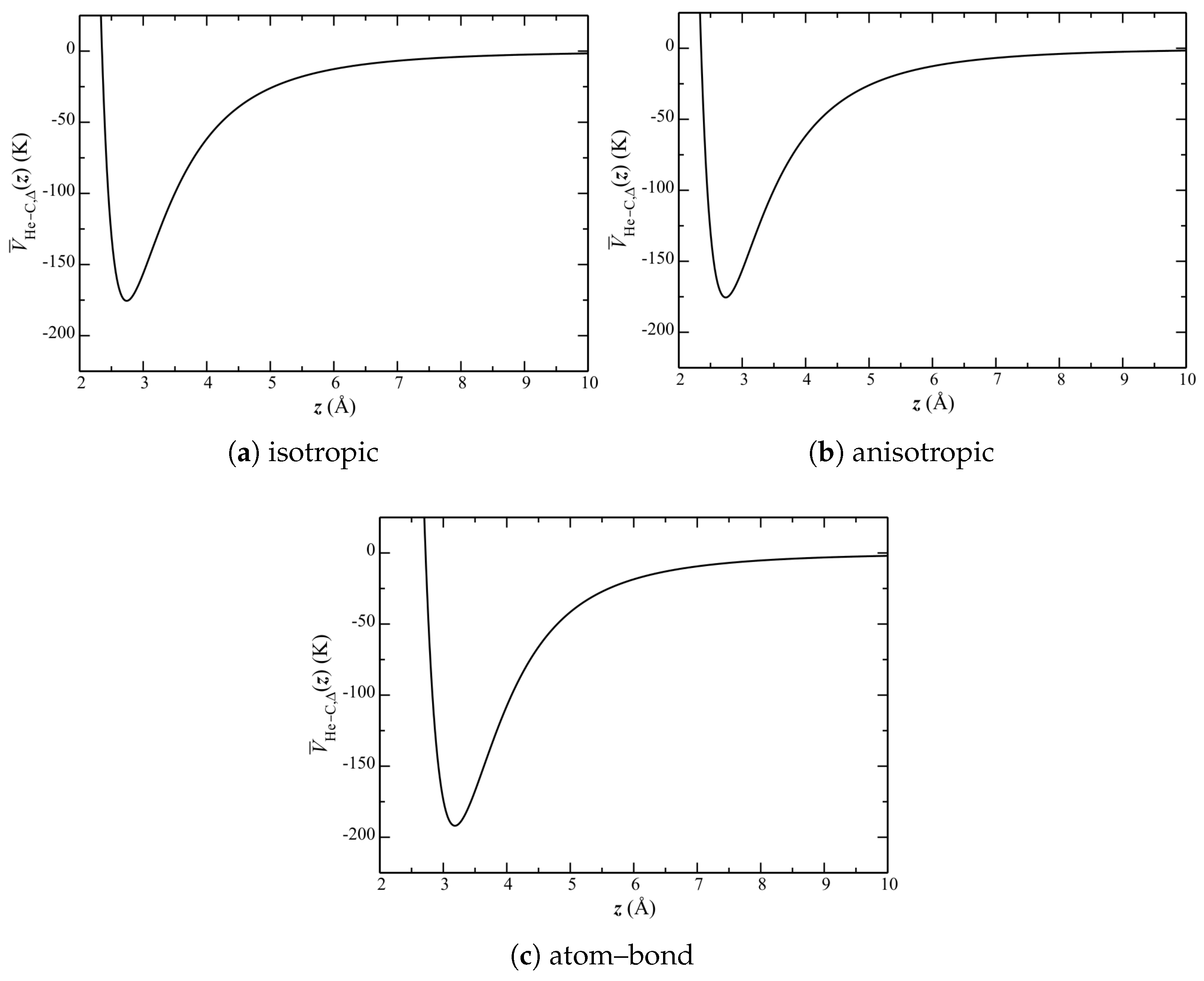
The separation of ${}^4$He atoms and their distribution is calculable directly from the simulations (and presented below). It is insightful, however, to first consider a single-body Schrödinger equation, with a potential ${\overline{V}}_{\mathrm{He}\text{–}\mathrm{C},△}$$\left(z\right)$ obtained as a lateral ($xy$) average (i.e., at each z) of $V_{\mathrm{He}\text{–}\mathrm{C}}$$\left(z\right)$ over the entire graphene plane.

Lateral-averaged potentials are shown in Figure 7. This side-by-side comparison shows that the isotropic and anisotropic potentials are qualitatively similar. The atom–bond potential, however, exhibits a much larger well depth, with a minimum at a much higher z.

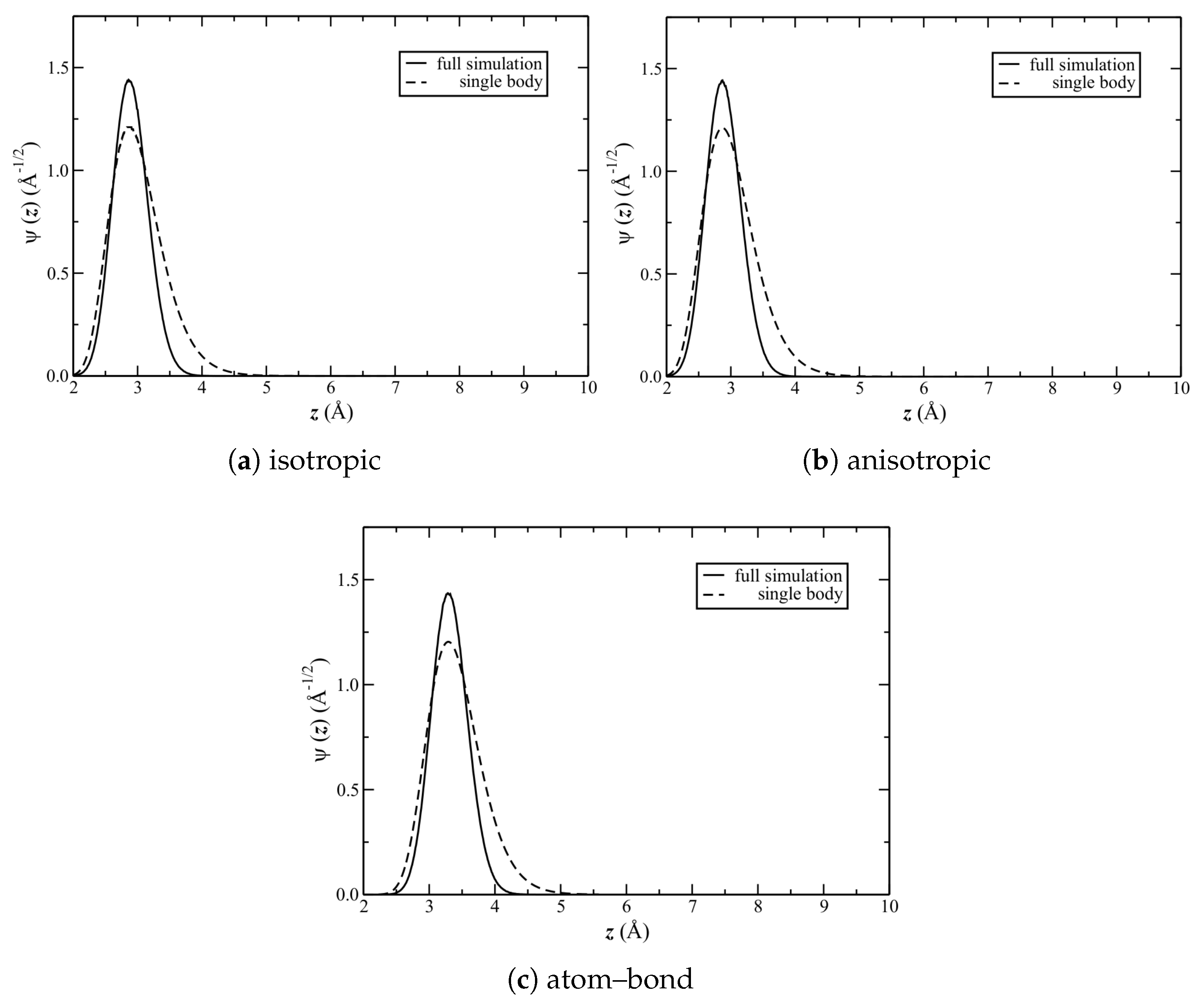
The solutions to the aforementioned Schrödinger equation for each of the potentials are shown in Figure 8. Shown also are full-simulation results, calculated at the equilibrium liquid densities (Table 2); note that the same $z_{\mathrm{e}}$ resulted also from calculating at the density of the $C_{1/3}$ structure (start of Section 3). The corresponding $z_{\mathrm{e}}$ and full width at half maximum (FWHM) are reported in

Table 3. The equilibrium separation of ${}^4$He atom(s) from the graphene plane $z_{\mathrm{e}}$, and the full width at half maximum (FWHM) of the associated distribution. Both single-body and full-simulation results are reported.

(a) single body			(b) full simulation
$\mathbf{V}$${}_{\mathbf{He}-\mathbf{C}}$	${\mathbf{z}}_{\mathbf{e}}$ (Å)	FWHM (Å)	${\mathbf{z}}_{\mathbf{e}}$ (Å)	FWHM (Å)
isotropic	$2.87$	$0.91$	$2.86$	$0.64$
anisotropic	$2.87$	$0.91$	$2.87$	$0.64$
atom–bond	$3.29$	$0.91$	$3.28$	$0.64$

.

First compare the single-body to full-simulation results. The latter are significantly more narrow (quantitatively, given by the FWHM). Figure 8 shows that the distributions are also (the most) different for $z>z_{\mathrm{e}}$. $z_{\mathrm{e}}$, however, as calculated by the two methods, are nearly identical. Consider now the difference between potentials. Interestingly, the FWHM is identical among them. This suggests that the shapes of the average potential wells (at least near the minima) are similar; and, hence, so is the average corrugation. $z_e$ is also the same for the isotropic and anisotropic potentials. It is significantly larger, however, for the atom–bond potential.

Consider now though the potential $V_{\mathrm{He}\text{–}\mathrm{C}}$($z_e$) (i.e., at the equilibrium separation) over the three symmetric sites (Figure 1b). The relative difference in potential at each of these sites represents the corrugation (defined above) felt by a ${}^4$He atom. These values are reported in

Table 4. Relative difference in $V_{\mathrm{He}\text{–}\mathrm{C}}$$\left(z\right)$ between the three symmetric sites (Figure 1b). Results are reported at $z=z_{\mathrm{e}}$ (Table 3b). Results are reported only to two decimal places.

V${}_{\mathbf{He}-\mathbf{C}}$	${\mathit{V}}_{\mathbf{top}}-{\mathit{V}}_{\mathbf{hollow}}$ (K)	${\mathit{V}}_{\mathbf{bridge}}-{\mathit{V}}_{\mathbf{hollow}}$ (K)	${\mathit{V}}_{\mathbf{top}}-{\mathit{V}}_{\mathbf{bridge}}$ (K)
isotropic	$9.31$	$7.93$	$1.38$
anisotropic	$15.60$	$13.29$	$2.31$
atom–bond	$5.56$	$4.93$	$0.63$

, and differences relative to the lateral averages are shown in

Table 5. The difference between $V_{\mathrm{He}\text{–}\mathrm{C}}$$\left(z_{\mathrm{e}}\right)$ and its lateral average ${\overline{V}}_{\mathrm{He}\text{–}\mathrm{C},△}$$\left(z_{\mathrm{e}}\right)$.

V${}_{\mathbf{He}-\mathbf{C}}$	${\overline{\mathit{V}}}_{\mathbf{He}\text{–}\mathbf{C},△}$$-{\mathit{V}}_{\mathbf{hollow}}$ (K)	${\overline{\mathit{V}}}_{\mathbf{He}\text{–}\mathbf{C},△}$$-{\mathit{V}}_{\mathbf{bridge}}$ (K)	${\overline{\mathit{V}}}_{\mathbf{He}\text{–}\mathbf{C},△}$$-{\mathit{V}}_{\mathbf{top}}$ (K)
isotropic	$5.86$	$-2.07$	$-3.45$
anisotropic	$9.89$	$-3.40$	$-5.71$
atom–bond	$4.19$	$-0.74$	$-1.37$

. There is a clear trend revealed by this table. The atom–bond potential is the least corrugated, followed by the isotropic and then (most significantly) anisotropic ones.

Finally, consider these results in the context of the phase diagram (Figure 5). Stronger corrugation leads to a lower equilibrium liquid density (Table 2). Regarding the stability of the $C_{1/3}$ structure, the deeper the (relative) well depth at an adsorption site (the hollow site; see Section 1), the harder it is to remove an atom (i.e., the more stable the solid). In this context, the results in Table 4 are also consistent with Figure 5. Differences on the order of kelvins therefore lead to significant quantitative changes in the phase diagram. This is despite the fact that well depths (at other z) are much deeper. Note that making more quantitative statements based only on $z_{\mathrm{e}}$ is probably not possible.

For the remainder of (this) Section 3, results based on the isotropic He–C potential are shown (unless otherwise stated). In Section 4, it is argued that this potential is the most accurate, though caution is needed.

3.3. Graphite

Nearly all experimental studies of ${}^4$He adsorbed on or scattered from a carbon surface are for graphite. All of the results presented earlier in this section, however, were for graphene. It is natural to ask whether these results can therefore be compared to experiment (as will be done in Section 4). It is also natural to ask the converse, of whether a He–C potential developed for graphite (such as the isotropic and anisotropic ones; see Section 2) might be inaccurate for studying adsorption on graphene.

${}^4$He adsorbed on graphite has been considered in prior calculations [5,6,11,12,13,14,15]. Because of this, and the fact that changing the He–He interaction will likely lead only to minor quantitative changes in the phase diagram (Section 3.1), results for these potentials are not (re-)reported in this section. Instead, quantitative details about the corrugation of the isotropic potential (only; see the remarks at the end of Section 3.2) are considered in the context of this prior work. This, however, motivates once more consideration of the atom–bond potential. Note that throughout this section, for one graphene layer, $N_{\mathrm{layers}}=1$, the results are repeated from Section 3.2. Note also that $N_{\mathrm{layers}}\ge 2$ is referred to as “graphite”.

A representative and recent prior study using the isotropic potential is that of [5]. Therein, it was found that the phase diagrams of graphene and graphite are qualitatively similar.

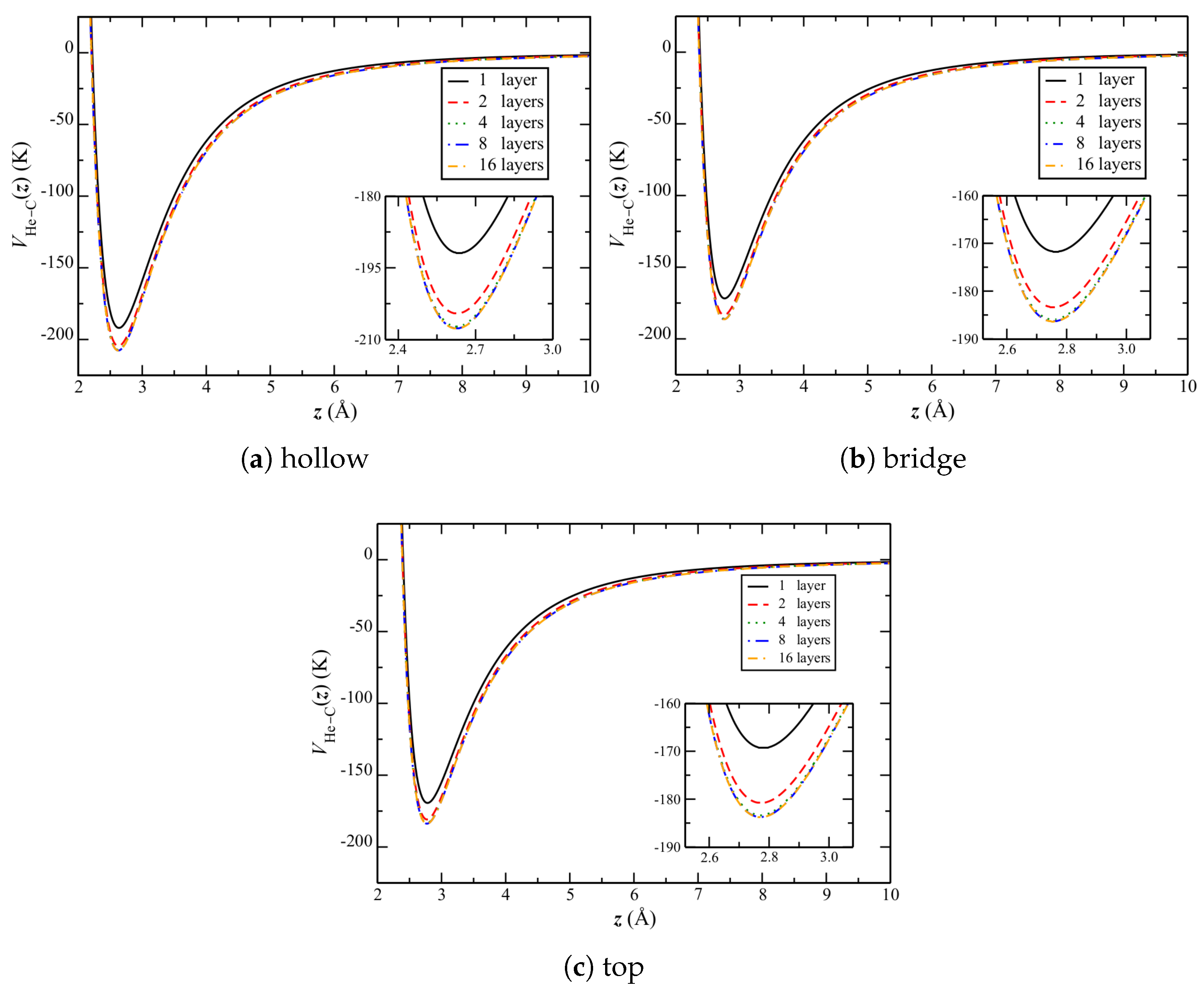
In order to understand this result, consider the changes in corrugation when going from graphene to graphite. Figure 9 shows the change in He–C potential over the three symmetric sites of the top graphene layer (Figure 1b), as the number of layers is increased. Qualitatively, the potential appears to uniformly decrease.

For the equilibrium separations reported in

Table 6. $z_{\mathrm{e}}$ and FWHM for graphite. Results are reported for an increasing number of graphene layers $N_{\mathrm{layers}}$, up to 16. Note that results are reported only for the single-body solution (see Section 3.2).

${\mathit{N}}_{\mathbf{layers}}$	${\mathit{z}}_{\mathbf{e}}$ (Å)	FWHM (Å)
2	$2.86$	$0.89$
4	$2.855$	$0.89$
8	$2.855$	$0.89$
16	$2.855$	$0.89$

, more quantitative results are reported in

Table 7. Relative difference in $V_{\mathrm{He}\text{–}\mathrm{C}}$$\left(z\right)$ between the three symmetric sites over the top graphene layer (Figure 1b) of graphite. Results are reported at $z=z_{\mathrm{e}}$ (Table 6).

${\mathit{N}}_{\mathbf{layers}}$	${\mathit{V}}_{\mathbf{top}}-{\mathit{V}}_{\mathbf{hollow}}$ (K)	${\mathit{V}}_{\mathbf{bridge}}-{\mathit{V}}_{\mathbf{hollow}}$ (K)	${\mathit{V}}_{\mathbf{top}}-{\mathit{V}}_{\mathbf{bridge}}$ (K)
2	$9.31$	$7.93$	$1.38$
4	$9.59$	$8.17$	$1.42$
8	$9.59$	$8.17$	$1.42$
16	$9.59$	$8.17$	$1.42$

and

Table 8. The difference between $V_{\mathrm{He}\text{–}\mathrm{C}}$$\left(z_{\mathrm{e}}\right)$ and ${\overline{V}}_{\mathrm{He}\text{–}\mathrm{C},△}$$\left(z_{\mathrm{e}}\right)$.

${\mathit{N}}_{\mathbf{layers}}$	${\overline{\mathit{V}}}_{\mathbf{He}\text{–}\mathbf{C},△}$$-{\mathit{V}}_{\mathbf{hollow}}$ (K)	${\overline{\mathit{V}}}_{\mathbf{He}\text{–}\mathbf{C},△}$$-{\mathit{V}}_{\mathbf{bridge}}$ (K)	${\overline{\mathit{V}}}_{\mathbf{He}\text{–}\mathbf{C},△}$$-{\mathit{V}}_{\mathbf{top}}$ (K)
2	$5.85$	$-2.08$	$-3.46$
4	$6.03$	$-2.14$	$-3.56$
8	$6.03$	$-2.14$	$-3.56$
16	$6.03$	$-2.14$	$-3.56$

. There are two significant observations to make from these tables. One is that the potentials at the symmetric sites all become stronger relative to the lateral average (Table 8), with increased repulsion at the bridge and top sites and attraction at the hollow one, with an increasing number of layers. That is, the corrugation becomes stronger. The other is that the relative well depth at the hollow site increases significantly more than the repulsion at either of the other two sites.

Despite the above, there is relatively little change in the equilibrium separation of atoms (Table 6). This might be due to that there are more bridge and top sites, as compared to hollow ones.

Increasing corrugation suggests that the solid phase will possibly become (more) stabilized relative to the liquid. This would have the most significant (qualitative) change for the atom–bond potential (see Section 3.2).

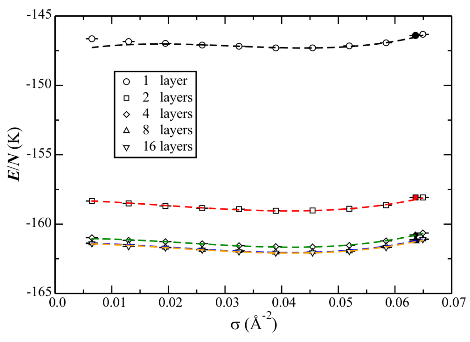
Motivated by this suggestion, the phase diagram calculated with the atom–bond potential, for an increasing number of layers, is shown in Figure 10. Corresponding data is reported in

Table 9. The corresponding data to Figure 10.

${\mathit{N}}_{\mathbf{layers}}$	${\mathit{\sigma }}_{\mathbf{eq}}$ (Å${}^{-2}$)	${\mathit{E}}_{\mathbf{l}}\left({\mathit{\sigma }}_{\mathbf{eq}}\right)$ (K)	${\mathit{E}}_{\mathbf{s}}\left({\mathit{\sigma }}_{\mathbf{s}}\right)$ (K)	${\mathit{E}}_{\mathbf{l}}\left({\mathit{\sigma }}_{\mathbf{s}}\right)$ (K)
1	$0.0413\left(7\right)$	$-147.32\left(3\right)$	$-146.401\left(9\right)$	$-146.79\left(9\right)$
2	$0.0417\left(5\right)$	$-159.05\left(1\right)$	$-158.20\left(1\right)$	$-158.25\left(9\right)$
4	$0.0418\left(5\right)$	$-161.67\left(2\right)$	$-160.78\left(1\right)$	$-160.86\left(9\right)$
8	$0.0416\left(6\right)$	$-162.05\left(1\right)$	$-161.117\left(9\right)$	$-161.21\left(9\right)$
16	$0.0417\left(6\right)$	$-162.09\left(2\right)$	$-161.21\left(1\right)$	$-161.26\left(9\right)$

. As suspected, the increased corrugation acts to stabilize the solid. Whereas for graphene the liquid remains the ground state at the density of the solid, the addition of even one layer causes the energies to be within error bars. Note that this situation then does not change (e.g., the solid eventually becoming the ground state), with an increasing number of layers, within the uncertainties of the calculations. The interpretation (for this He–C potential) could be that the liquid is stable as the ground-state on graphite, until reaching the density of the solid, where they are then in equilibrium.

4. Discussion

The phase diagrams of ${}^4$He adsorbed on graphene and graphite were calculated; the results are presented in Section 3. Particular focus was placed on the importance of the He–He (Section 3.1) and He–C (Section 3.2) interactions. By careful consideration also of other approximations and convergence (see Section 2), the simulations are otherwise (numerically) exact.

The He–He interaction (Section 3.1) was found to have only a quantitative effect on the phase diagram (for the pairwise potentials considered). The He–C interaction (Section 3.2), however, had much more significant and both qualitative and quantitative effects. The results were found to be relatively insensitive to the consideration of graphene (Section 3.1 and Section 3.2) or graphite (Section 3.3). They are therefore discussed non-specifically below.

Assuming the validity of the pairwise forms of these potentials (see Section 2), for the moment, their accuracy may be assessed through comparison to both experiment and first-principles data.

Consider first the comparison to experiment. Several properties of the phase diagram can be compared. The equilibrium liquid density has been determined from heat-capacity measurements [19], and is about $0.04$ Å${}^{-2}$. While the phase diagrams (Figure 3) for the He–He potentials of Aziz and Przybytek et al. are similar, the latter is in better quantitative agreement (Table 1) with this. Considering therefore only the latter potential for this discussion, it is found (Section 3.2) that only the isotropic and atom–bond He–C potentials are consistent with this (Table 2). The anisotropic potential, however, does not lead to a ground-state liquid, and has an equilibrium liquid density that is much too low.

Another property that can be compared is the equilibrium separation of atoms. Both the isotropic and anisotropic He–C potentials agree very well (Table 6) with the experimental value of $z_e=2.85$ Å [36]. $z_e$ for the atom–bond potential, however, is much too large.

The stability of the $C_{1/3}$ structure is a well-established feature of the experimental phase diagram (as discussed in Section 1). The atom–bond potential, however, does not exhibit an unambiguous stable solid phase. Even for the case of graphite (Section 3.3), for which the solid and the liquid are in equilibrium, it is likely that corrections to the remaining approximations (see below) would destabilize the solid.

There is also the experimental possibility of an equilibrium between the liquid and $C_{1/3}$ structure [19]. While none of the considered He–C potentials are consistent with this possibility, corrections to the remaining approximations (see below) may lead to this, by “softening” the interactions.

In addition to the phase diagram, it is also possible to compare binding energies. These are known from scattering experiments [37]. Computationally, these are computed as the energy levels of the single-body Schrödinger equation (as discussed in Section 3.2). For graphite, this has already been done for the isotropic and anisotropic [29] and atom–bond [23] potentials. The former two give similar results, with all values slightly underestimated. The latter overestimates them, most significantly for the lowest energy levels.

The above comparisons provide important insight into the approximations to the He–C interaction. Consider, in particular, the corrugation. That of the atom–bond potential is much too weak; the isotropic one is a bit too strong; and, finally, that of the anisotropic one is much too strong.

The above insight is consistent with comparisons to first-principles data [23]. While the atom–bond potential, for example, is quite accurate for the bridge and top sites (Figure 1b), it significantly underestimates the well depth for the hollow one. Note that the importance of this would also impact the potential at the equilibrium separation of atoms. The statements above for the relative differences in the isotropic and anisotropic potentials are also consistent with this.

All of the interactions considered assume that the He–He and He–C interactions can be approximated separately and by a sum of pairwise potentials (Section 2). An important consideration is therefore the extent to which many-body effects play a role. Note that with consideration of a fixed carbon lattice, and the interpretation of the He–C potential as that of a ${}^4$He atom with the entire carbon lattice (Section 2), such “many-body effects” refer to the addition of a ${}^4$He atom(s) to the above interactions.

Consider first the many-body effects in the He–He interaction. The first correction to this would be that of He–He–He. The aforementioned (Section 2) recent evaluation [28] of different He–He potentials found, for three considered models of three-body interactions, that the effect for ${}^4$He${}_3$ was less than $0.001$ K. It therefore seems unlikely that there would be quantitative changes to the results reported herein, based on this or higher-order interactions.

Another consideration is the many-body effects related to the He–C interaction, the first correction being that of He–He–C; in other words, a substrate-mediated change in the He–He interaction. A standard approximation to this, meaningful for graphite, is given by the so-called McLachlan interaction [38]. This has also been considered in prior work [5] (see also Section 3.2). Based on this, the energy of the liquid at its equilibrium density is increased by $0.20\left(1\right)$ K, while that of the solid is increased by $0.37\left(1\right)$ K. Assuming that the former can be considered as a uniform shift in the liquid curve of the phase diagram, it can be qualitatively said that this correction would soften the He–He interaction, and destabilize the solid.

Quantitatively, the many-body corrections to the He–C interaction would be enough to play an important role in the phase diagram. Even a relative shift in the stability of the solid by $0.17\left(1\right)$ K, based on the above discussion, would be enough to make the liquid the equilibrium ground-state for the isotropic potential (see Table 2), and lead to a coexistence region with the solid [19].

5. Conclusions

The phase diagrams of ${}^4$He adsorbed on graphene and graphite were calculated using quantum simulation methods. By careful consideration of convergence, the methods used (Section 2) are (numerically) exact up to the approximations of the He–He and He–C interactions (and the adiabatic approximation). These were investigated in detail in Section 3 and Section 4.

The results were shown to be qualitatively insensitive to the form of modern pairwise He–He potentials, which has now been calculated and fit to an analytical form (Przybytek et al.) with high accuracy. Quantitatively, however, the results (Section 3.1) are slightly improved (Section 4). It was discussed (Section 4) that many-body effects are not likely to change this.

The He–C interaction, however, plays a significant role both qualitatively and quantitatively. Modern pairwise potentials all give significantly different results (Section 3.2). Consider first though that such potentials do all give similar lateral-averaged shapes (Figure 7). Therefore, the average corrugation, irrespective of the potential, seems correct. The phase diagram (Figure 5), however, depends significantly on the choice of potential. Based on the discussion in Section 4, it seems clear that the corrugation of the anisotropic potential is much too strong, and that of the atom–bond potential too weak. The isotropic potential is also a bit too strong, although it seems to be the most accurate. Many-body effects though are also expected (Section 4) to play an important quantitative role. Details on the corrugation and many-body effects seem to be needed on the order of kelvins. This is far below the accuracy of modern approximations to the He–C interaction.

Only phase diagrams were considered in this work. Not considered, for example, were properties of the systems. A notable example is superfluidity, and its possible leading to a supersolid phase (as discussed in Section 1). Quantitative accuracy for such properties may be even more challenging than for the phase diagram though, because of sensitivities to the He–He and He–C interactions. Therefore, considering them without a more accurate He–C interaction hardly seems worthwhile.

Looking forward, it is clear that what is needed is a better understanding of and a more accurate approximation to the He–C interaction. This includes both in the pairwise interaction between a helium atom and the carbon surface, and any substrate-mediated change in the He–He interaction. Treating the carbon atoms quantum mechanically [10] will also be important. Only with these considerations can quantitatively meaningful statements be made. These will be the subjects of future work.

References

- Cazorla, C.; Boronat, J. Simulation and understanding of atomic and molecular quantum crystals. Rev. Mod. Phys. 2017, 89, 035003. [Google Scholar] [CrossRef]
- McMahon, J.M.; Morales, M.A.; Pierleoni, C.; Ceperley, D.M. The properties of hydrogen and helium under extreme conditions. Rev. Mod. Phys. 2012, 84, 1607–1653. [Google Scholar] [CrossRef]
- Boninsegni, M.; Prokof’ev, N.V. Colloquium: Supersolids: What and where are they? Rev. Mod. Phys. 2012, 84, 759–776. [Google Scholar] [CrossRef]
- Zimmerli, G.; Mistura, G.; Chan, M.H.W. Third-sound study of a layered superfluid film. Phys. Rev. Lett. 1992, 68, 60–63. [Google Scholar] [CrossRef] [PubMed]
- Gordillo, M.C.; Boronat, J. 4He on a Single Graphene Sheet. Phys. Rev. Lett. 2009, 102, 085303. [Google Scholar] [CrossRef] [PubMed]
- Gordillo, M.C.; Cazorla, C.; Boronat, J. Supersolidity in quantum films adsorbed on graphene and graphite. Phys. Rev. B 2011, 83, 121406. [Google Scholar] [CrossRef]
- Kwon, Y.; Ceperley, D.M. 4He adsorption on a single graphene sheet: Path-integral Monte Carlo study. Phys. Rev. B 2012, 85, 224501. [Google Scholar] [CrossRef]
- Happacher, J.; Corboz, P.; Boninsegni, M.; Pollet, L. Phase diagram of 4He on graphene. Phys. Rev. B 2013, 87, 094514. [Google Scholar] [CrossRef]
- Gordillo, M.; Boronat, J. Phase Diagrams of 4He on Flat and Curved Environments. J. Low Temp. Phys. 2013, 171, 606–612. [Google Scholar] [CrossRef] [Green Version]
- Gordillo, M.C. Diffusion Monte Carlo calculation of the phase diagram of 4He on corrugated graphene. Phys. Rev. B 2014, 89, 155401. [Google Scholar] [CrossRef]
- Gottlieb, J.M.; Bruch, L.W. Ground state of monolayer 4He/graphite: Quantum liquid versus quantum solid. Phys. Rev. B 1993, 48, 3943–3948. [Google Scholar] [CrossRef]
- Whitlock, P.A.; Chester, G.V.; Krishnamachari, B. Monte Carlo simulation of a helium film on graphite. Phys. Rev. B 1998, 58, 8704–8715. [Google Scholar] [CrossRef]
- Pierce, M.E.; Manousakis, E. Monolayer Solid 4He Clusters on Graphite. Phys. Rev. Lett. 1999, 83, 5314–5317. [Google Scholar] [CrossRef]
- Pierce, M.E.; Manousakis, E. Role of substrate corrugation in helium monolayer solidification. Phys. Rev. B 2000, 62, 5228–5237. [Google Scholar] [CrossRef]
- Corboz, P.; Boninsegni, M.; Pollet, L.; Troyer, M. Phase diagram of 4He adsorbed on graphite. Phys. Rev. B 2008, 78, 245414. [Google Scholar] [CrossRef]
- Bretz, M.; Dash, J.G.; Hickernell, D.C.; McLean, E.O.; Vilches, O.E. Phases of He3 and He4 Monolayer Films Adsorbed on Basal-Plane Oriented Graphite. Phys. Rev. A 1973, 8, 1589–1615. [Google Scholar] [CrossRef]
- Bretz, M.; Dash, J.G.; Hickernell, D.C.; McLean, E.O.; Vilches, O.E. Erratum: Phases of He3 and He4 monolayer films adsorbed on basal-plane oriented graphite. Phys. Rev. A 1974, 9, 2814–2814. [Google Scholar] [CrossRef]
- Carneiro, K.; Ellenson, W.D.; Passell, L.; McTague, J.P.; Taub, H. Neutron-Scattering Study of the Structure of Adsorbed Helium Monolayers and of the Excitation Spectrum of Few-Atomic-Layer Superfluid Films. Phys. Rev. Lett. 1976, 37, 1695–1698. [Google Scholar] [CrossRef]
- Greywall, D.S.; Busch, P.A. Heat capacity of fluid monolayers of 4He. Phys. Rev. Lett. 1991, 67, 3535–3538. [Google Scholar] [CrossRef] [PubMed]
- Crowell, P.A.; Reppy, J.D. Reentrant superfluidity in 4He films adsorbed on graphite. Phys. Rev. Lett. 1993, 70, 3291–3294. [Google Scholar] [CrossRef] [PubMed]
- Przybytek, M.; Cencek, W.; Komasa, J.; ach, G.; Jeziorski, B.; Szalewicz, K. Relativistic and Quantum Electrodynamics Effects in the Helium Pair Potential. Phys. Rev. Lett. 2010, 104, 183003. [Google Scholar] [CrossRef] [PubMed]
- Przybytek, M.; Cencek, W.; Komasa, J.; ach, G.; Jeziorski, B.; Szalewicz, K. Erratum: Relativistic and Quantum Electrodynamics Effects in the Helium Pair Potential [Phys. Rev. Lett. 104, 183003 (2010)]. Phys. Rev. Lett. 2012, 108, 129902. [Google Scholar] [CrossRef]
- Bartolomei, M.; Carmona-Novillo, E.; Hernández, M.I.; Campos-Martínez, J.; Pirani, F. Global Potentials for the Interaction between Rare Gases and Graphene-Based Surfaces: An Atom–Bond Pairwise Additive Representation. J. Phys. Chem. C 2013, 117, 10512–10522. [Google Scholar] [CrossRef]
- Born, M. Die Gültigkeitsgrenze der Theorie der idealen Kristalle und ihre Überwindung. In Festschrift zur Feier des Zweihundertjährigen Bestehens der Akademie der Wissenschaften in Göttingen; Springer: Berlin/Heidelberg, Germany, 1951; pp. 1–16. [Google Scholar]
- Aziz, R.A.; Chen, H.H. An accurate intermolecular potential for argon. J. Chem. Phys. 1977, 67, 5719–5726. [Google Scholar] [CrossRef]
- Aziz, R.A.; Janzen, A.R.; Moldover, M.R. Ab Initio Calculations for Helium: A Standard for Transport Property Measurements. Phys. Rev. Lett. 1995, 74, 1586–1589. [Google Scholar] [CrossRef] [PubMed]
- Cencek, W.; Przybytek, M.; Komasa, J.; Mehl, J.B.; Jeziorski, B.; Szalewicz, K. Effects of adiabatic, relativistic, and quantum electrodynamics interactions on the pair potential and thermophysical properties of helium. J. Chem. Phys. 2012, 136, 224303. [Google Scholar] [CrossRef] [PubMed]
- Stipanović, P.; Markić, L.V.; Boronat, J. Elusive structure of helium trimers. J. Phys. B At. Mol. Opt. Phys. 2016, 49, 185101. [Google Scholar] [CrossRef]
- Carlos, W.E.; Cole, M.W. Interaction between a He atom and a graphite surface. Surf. Sci. 1980, 91, 339–357. [Google Scholar] [CrossRef]
- Pirani, F.; Albertí, M.; Castro, A.; Teixidor, M.M.; Cappelletti, D. Atom–bond pairwise additive representation for intermolecular potential energy surfaces. Chem. Phys. Lett. 2004, 394, 37–44. [Google Scholar] [CrossRef]
- Pirani, F.; Cappelletti, D.; Liuti, G. Range, strength and anisotropy of intermolecular forces in atom–molecule systems: an atom–bond pairwise additivity approach. Chem. Phys. Lett. 2001, 350, 286–296. [Google Scholar] [CrossRef]
- Needs, R.J.; Towler, M.D.; Drummond, N.D.; Ríos, P.L. Continuum variational and diffusion quantum Monte Carlo calculations. J. Phys. Condens. Matter 2010, 22, 023201. [Google Scholar] [CrossRef] [PubMed]
- Cazorla, C.; Astrakharchik, G.E.; Casulleras, J.; Boronat, J. Bose–Einstein quantum statistics and the ground state of solid 4He. New J. Phys. 2009, 11, 013047. [Google Scholar] [CrossRef]
- Cazorla, C.; Astrakharchik, G.E.; Casulleras, J.; Boronat, J. Ground-state properties and superfluidity of two- and quasi-two-dimensional solid 4He. J. Phys. Condens. Matter 2010, 22, 165402. [Google Scholar] [CrossRef] [PubMed]
- Pillai, M.; Goglio, J.; Walker, T.G. Matrix Numerov method for solving Schrödinger’s equation. Am. J. Phys. 2012, 80, 1017–1019. [Google Scholar] [CrossRef]
- Carneiro, K.; Passell, L.; Thomlinson, W.; Taub, H. Neutron-diffraction study of the solid layers at the liquid-solid boundary in 4He films adsorbed on graphite. Phys. Rev. B 1981, 24, 1170–1176. [Google Scholar] [CrossRef]
- Ruiz, J.; Scoles, G.; Jonsson, H. On the laterally averaged interaction potential between He atoms and the (0001) surface of graphite. Chem. Phys. Lett. 1986, 129, 139–143. [Google Scholar] [CrossRef]
- McLachlan, A. Van der Waals forces between an atom and a surface. Mol. Phys. 1964, 7, 381–388. [Google Scholar] [CrossRef]
Figure 1.
(a) A cutaway of graphene and adsorbed helium atoms. A single layer is shown, but up to 16 (as an approximation to graphite) are considered in this work. (b) High-symmetry sites over the graphene plane. These will be referred to as the hollow, bridge, and top sites. Note that these results were calculated using the helium–helium (He–He) potential of Przybytek et al. and the isotropic helium–carbon (He–C) potential (discussed in Section 2).
Figure 2.
Density plots of (a) the liquid, at the equilibrium density, and (b) solid () phases. See the text for (general) details. Note that these results were calculated using the He–He potential of Przybytek et al. and the isotropic He–C potential.
Figure 3.
Phase diagram of He adsorbed on graphene. Energies E per particle (abbreviated as ) as a function of (surface) density are shown for the two He–He potentials under consideration.
Figure 4.
The He–He potential as a function of pairwise separation r. The insets in (a,b) show expanded views of the minima; and (c) shows the difference between potentials, , with the inset showing an expanded view of the region near and just above the minima.
Figure 5.
Phase diagram of He adsorbed on graphene. Results are shown for the three He–C potentials under consideration. Open circles correspond to liquid data, the dashed lines are fits to this data (Equation (6)), and filled circles correspond to the phase. Note that (a) is the same as in Figure 3b.
Figure 6.
The He–C potential as a function of height z over the three symmetric sites of the graphene plane (Figure 1b). The insets show expanded views of the minima.
Figure 7.
Lateral-averaged He–C potential .
Figure 8.
(from Equation (5)). Both single-body and full-simulation results are shown.
Figure 9.
over the three symmetric sites of the top graphene layer (Figure 1b) of graphite. Results are shown for increasing numbers of graphene layers, up to 16.
Figure 10.
Phase diagram of He adsorbed on graphite. Note that these results were calculated using the atom–bond He–C potential.