Smeared Lattice Model as a Framework for Order to Disorder Transitions in 2D Systems


1
Military Academy of the Republic of Belarus, Minsk 220057, Belarus
2
Institute for Nuclear Problems, Belarus State University, Minsk 220050, Belarus
*
Author to whom correspondence should be addressed.
Crystals 2018, 8(7), 290; https://doi.org/10.3390/cryst8070290
Submission received: 15 June 2018
/
Revised: 11 July 2018
/
Accepted: 12 July 2018
/
Published: 14 July 2018
(This article belongs to the Special Issue Selected Papers from "The 1st International Electronic Conference on Crystals")
Abstract
:Order to disorder transitions are important for two-dimensional (2D) objects such as oxide films with cellular porous structure, honeycomb, graphene, Bénard cells in liquid, and artificial systems consisting of colloid particles on a plane. For instance, solid films of porous alumina represent almost regular crystalline structure. We show that in this case, the radial distribution function is well described by the smeared hexagonal lattice of the two-dimensional ideal crystal by inserting some amount of defects into the lattice.Another example is a system of hard disks in a plane, which illustrates order to disorder transitions. It is shown that the coincidence with the distribution function obtained by the solution of the Percus–Yevick equation is achieved by the smoothing of the square lattice and injecting the defects of the vacancy type into it. However, better approximation is reached when the lattice is a result of a mixture of the smoothed square and hexagonal lattices. Impurity of the hexagonal lattice is considerable at short distances. Dependencies of the lattice constants, smoothing widths, and contributions of the different type of the lattices on the filling parameter are found. The transition to order looks to be an increase of the hexagonal lattice fraction in the superposition of hexagonal and square lattices and a decrease of their smearing.
1. Introduction
It is well known that for particles on a plane interacting via a certain potential, the existence of a periodic crystal is impossible at nonzero temperature [1,2,3,4]. However, there exist a number of two-dimensional (2D) objects in nature that exhibit crystalline-like ordering. Usually these objects have nonperfect crystalline structure, and a question arises about transition from order to disorder. It is noteworthy that the order–disorder transition was experimentally studied from the general point of view in [5], where the destruction of a graphene layer by electron beam was investigated. A continuous transition from the crystalline state to the glassy state occurred as a result of irradiation. At the initial stage of irradiation, individual defects appeared in the lattice. Then, the glassy (disordered) regions surrounding crystallites (perfectly oriented regions) emerged. In the disordered regions, the destruction of the order initially manifested itself as pentagonal and heptagonal cells instead of hexagonal ones. The area occupied by crystallites decreased with an increase in the irradiation dose.
As was believed in [5], the experiment confirmed the validity the two competing theories of the order–disorder transition. They involve, on the one hand, the theory of crystallites [6], according to which an amorphous substance incorporates crystal-like agglomerates linked by disordered regions, and, on the other hand, the theory of random networks (see review [7]), which assumes that the order is destroyed throughout the entire volume of a substance, so that the crystal lattice transforms into random chains of atoms due to the distortion and breakage of some bonds. Thus, it follows from the experiment in [5] that single defects are formed at the initial stages. Then the theory of crystallites proves to be valid; further, the theory of random networks starts to work. We propose to take into consideration two mechanisms in order to simulate the radial distribution function of 2D systems. The first one implies the formation of vacancy-type defects (i.e., the absence of atoms in some lattice sites) while the crystal lattice structure is retained. The second mechanism corresponds to the destruction of the crystal lattice and is implemented via peak broadening in the structure factor and limitation of the peak height at large wave numbers. The method of crystal lattice smearing was used to construct an empirical radial distribution function [8]. This method was applied to describe the structure of some simple liquids [9,10,11,12,13,14,15]. A similar method of smearing of coordinate circles was used to describe artificial 2D crystals [16,17]. Here we consider a slightly different method consisting in the random shifting of the crystal nodes.
2. Radial Distribution Function for Porous Aluminum Oxide Layer
Oxide films with a cellular porous structure are formed upon the electrochemical oxidation (anodization) of aluminum and many aluminum alloys in solutions of various acids. The film thickness may be as large as hundreds of micrometers, while the pore radius size is tens of nanometers. Such films have been studied for more than 50 years. They are widely applied as anticorrosion, wear-resistant, electro-insulating, and decorative coatings in microelectronic and optical devices, membranes, and sensors. Under a combination of certain conditions, including acid concentration and type, a film can be grown as an ordered array of cylindrical pores similar to a 2D periodic lattice [18,19,20]. Various theories describing the ordered structure of pores in aluminum oxide fabricated by anodization have been proposed [21,22]. However, presently there is no complete understanding of the regularities of ordered structure formation, hence the radial distribution function of pores cannot be calculated theoretically. At the same time, knowledge of the radial distribution function is necessary for optical calculations. For example, the effective refractive index of a medium consisting of porous aluminum oxide depends strongly on the radial distribution function [23]. The imaginary part of the effective refractive index is particularly sensitive to the form of the radial distribution function. As for the experimental determination of the radial distribution function using an electron microscope, its accuracy is limited by finite sample sizes [24]. Thus, one needs semi-empirical models to describe the radial distribution function of pores in porous aluminum oxide. It is reasonable to suggest that the ordered structure of porous aluminum oxide is something intermediate between the 2D crystal and an amorphous substance. Therefore, it is meaningful to study porous aluminum oxide from the viewpoint of general principles of the order–disorder transition [25,26].
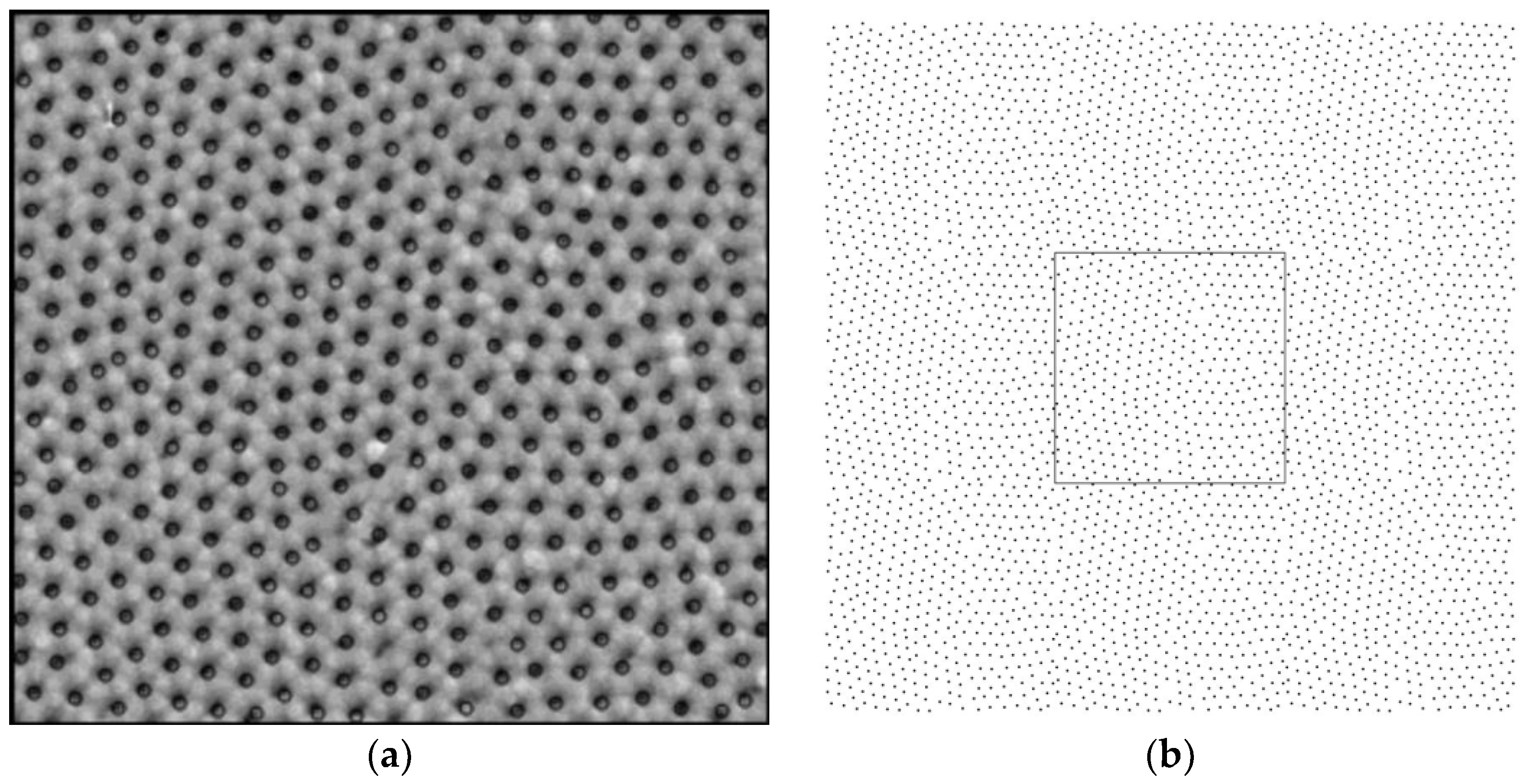
Let us first analyze a real sample of porous aluminum oxide in order to understand the form of the radial distribution function that we should seek. In practice, there is generally a photograph of the sample that can be analyzed by statistical methods [24]. In this study, we used the electron microscopy image obtained in [27], shown in Figure 1a. There are computer programs that can determine the centers of cylindrical holes [24], which analyze the contrast of pixels. However, we plotted the pore centers manually. The average distance between pores in the sample was on the order of 100 nm [27]. To avoid edge effects and at the same time have an opportunity to calculate the radial correlation function at somewhat larger distances, we increased the sample area by parallel translations along the coordinate axes and diagonals (Figure 1b). Although this increase in area gave rise to a certain error, it allowed us to increase the distance at which the correlation function can be calculated. Then, using a computer program, we counted the number of pores between the circles of radii and (including the pores of the extended sample) in the neighborhood of each selected pore of the initial sample. Such calculation was performed for each pore of the initial sample, and then the average value was found. A binary distribution function of the pore density distribution was calculated by the formula
where is the number of pores in the region between the circles of radii and , and is the number of pores in the sample. The correction factor in Equation (1) takes into account the fact that the selected pore cannot be situated within its environment. The radial distribution function related to the function by the expression is usually used, where is the average surface density of pores in the sample. Thus, the calculation of the radial distribution function is similar to the calculation in the Monte Carlo method, except for the fact that the sample in the Monte Carlo method is generated, while the method at hand deals with an experimental sample. In this way, the radial distribution function was obtained. However, the statistical uncertainty and the error due to edge effects restrict the direct use of this function for optical calculations, since they give rise to errors in the calculation of integrals. At the same time, this accuracy is quite sufficient to construct an empirical distribution function to compare with the experimental one. A further objective of our study was to derive a smooth empirical distribution function that could be used in optical calculations. A starting point of our approach is the binary distribution function of particles for an ideal 2D crystal with a certain hexagonal lattice, shown in Figure 2a. The crystal structure is described, e.g., in [16,25,26]. The two-particle distribution function is a sum of the Dirac delta-function terms:
where represents a two-dimensional delta function by Dirac, and are position vectors of particles in an ideal lattice. The particles are situated in the nodes of the crystalline lattice. Summation in Equation (2) is performed over all the particles, except one, being in an origin of coordinates. As we have one particle per cell, an average density of the particles in an ideal crystal is easily calculated: where is an area of a crystal cell, is a lattice constant (i.e., diameter of a circle inscribed into the cell, as shown in Figure 2), and is the number of edges of a cell.
The correlation function is denoted as . To proceed from order (an ideal crystal) to disorder, we suggest forming the defects of the vacancy type at the first stage. This means there is a probability that a particle in a node will be lacking. As a result, the distribution function takes the form
where denotes a distribution function at this first stage, is the surface density of the particles in a sample, and is a distance at which it is known that the distribution function is apparently zero. Equation (3) suggests that the correlation function of an ideal crystal is exponentially restricted at large . Besides, it is taken into account that should have the correct asymptote at infinity, where it is equal to , and should be equal to zero at . At the second stage, the spreading of a lattice by means of some integral transformation is carried out:
where we suppose
The integral transformation given by Equations (4) and (5) maps a set of the integrable functions defined on a two-dimensional region into itself. At , , as in (3). Normalizing factor is equal to
where is a zero-order modified Bessel function of the first kind. The above expression for implies that the action of the transformation in Equation (4) to the function whose value is some constant does not change it. As a result, one comes to
We do not consider an orientation order and a loss of it here, and an averaged over orientation of the vector (polar coordinates are used) is considered. Thus, all the directions are equivalent, and the pare distribution function depends only on distance . As a result, we come to the following formula for :
where summation is performed not over the nodes, but over coordinate circles on which the nodes are situated, and is the number of nodes lying on each th coordinate circle.
3. Hard Disks in a Plane
Let us consider a quite different system, namely, hard disk fluid. This system, on the one hand, attracts mathematicians and physicists with its simplicity, while on the other hand, it is a test bed to explore transition from order to disorder, hard disc liquid to hexatic, liquid to hexagonal crystal, and liquid to maximally random jammed state [28,29,30,31,32]. The pair distribution function characterizes the important features of the system as compressibility and the equation of state [33,34]. The limiting case of a distribution function of hard disks under increasing disk concentration is the hexagonal lattice, i.e., a two-dimensional crystal. It is reasonable that at densities close to maximum, the two-particle distribution function can be described by the smearing of a hexagonal lattice. At lower concentrations of particles, the methods of integral equations [35], based on a decoupling of the Bogolubov chain of equations, work well. In particular, the Percus–Yevick integral equation [29,35] is usually used. The question arises as to whether the smeared lattice model works not only in proximity to a crystal, but also at medium concentrations. Below we consider this model at the range of medium concentration of disks.
Comparison with Solutions of the Percus–Yevick Equation
Disk concentration is characterized by the packing fraction , where is a disk radius. It is evident that , because the centers of the two hard disks are separated by at least this distance. The value of the lattice constant has to depend on . The question arises as to what lattice should be smeared to obtain the correct pair distribution function. It turns out that qualitative agreement with solutions of the Percus–Yevick equation is achieved if a square lattice is smeared. On the other hand, it is obvious that under increased disk density, we should come to a hexagonal lattice. To take this into account, we suggest the following model:
i.e., the radial distribution function is a superposition of two terms obtained by the spreading of square and hexagonal lattices with weight functions that depend on the distance. The functions and are calculated by Equation (8). The parameter determining spreading of the lattice depends on distance as ; that is, the nodes situated farther away are more strongly smeared. A comparison of the results with solutions of the Percus–Yevick equation is shown in Figure 4 and Figure 5. It should be noted that the Percus–Yevick equation is not analytically solved for hard disks on a plane, therefore numerical methods were used. It seems very interesting that the “tails” of the distribution function shown in Figure 4b and Figure 5b are modeled with high accuracy. The Percus–Yevick equation stops working when the filling parameter is greater than 0.63, which restricts the present analysis. However, it is evident that parameterization of the radial distribution function given by Equation (8) will be useful for higher disk concentrations, where phase transitions occur. Table 1 contains all the parameters used in the calculations. For simplicity, we assume that the parameters and determining smearing and some amount of defects/vacancies are the same for both lattices; however, the lattice constants are taken differently. As one can see, the spreading and number of defects decrease with increasing , i.e., the system tends to go from disorder to order. The interesting question is why the square lattice plays a major role in this range of packing fraction, and why the admixture of the triangle lattice shown in Figure 1c does not lead to a better coincidence.
4. Conclusions
Radial distribution function parameterization based on the smeared lattice model is presented. This parameterization describes the same footing as porous aluminum oxide and 2D hard disk fluid. The smeared lattice model is based on two effects: the first is the vacancy type of defect formation and the second is destruction of the crystal lattice by smearing. The success of this parameterization shows that even liquid of hard disks contains features of a crystal. The model will serve as a tool for a description of the phase transitions in 2D fluids. Variational methods [36] could be used to calculate the model parameters, such as spreading, probability of defects, and lattice constants by minimization of some function [36].
Author Contributions
Both of the Authors developed the theoretical model. Besides, N.L.C. analyzed the data for porous aluminum oxide layer and find numerical solution for the Percus–Yevick equation for hard disks in a plane.
Funding
The Authors ask European Physical Society (EPS) to support publication of this paper, but at the moment of this final version submission there is no EPS decision yet. If the EPS support will take place the Authors will be grateful to EPS. No other external funding was used for this research.
Conflicts of Interest
The authors declare no conflict of interest.
References
- Peierls, R.E. Transformation tempretures. Helv. Phys. Acta Suppl. 1934, 2, 81–83. [Google Scholar]
- Landau, L.D. On the theory of phase transitions I. Phys. Z. Sowjet. 1937, 11, 26–35. [Google Scholar] [CrossRef]
- Landau, L.D. On the theory of phase transitions II. Phys. Z. Sowjet. 1937, 11, 545–555. [Google Scholar]
- Mermin, N.D. Crystalline order in two dimensions. Phys. Rev. 1968, 176, 250–254. [Google Scholar] [CrossRef]
- Eder, F.R.; Kotakoski, J.; Kaiser, U.; Meyer, J.C. A journey from order to disorder—Atom by atom transformation from graphene to 2D carbon glass. Sci. Rep. 2014, 4, 4060. [Google Scholar] [CrossRef] [PubMed]
- Warren, B.E. X-ray Diffraction Study of the Structure of Glass. Chem. Rev. 1940, 26, 237–255. [Google Scholar] [CrossRef]
- Wright, A.C.; Thorpe, M.F. Eighty years of random networks. Phys. Status Solidi B 2013, 250, 931–936. [Google Scholar] [CrossRef]
- Prins, G.A.; Petersen, H. Theoretical diffraction patterns corresponding to some simple types of molecular arrangement in liquids. Physica 1936, 3, 147–153. [Google Scholar] [CrossRef]
- Glauberman, A.E. On the theory of a local order inliquids. Zh. Eksp. Teor. Fiz. 1952, 22, 249–250. [Google Scholar]
- Tsvetkov, V.P. About structure of the liquid metals. Izv. Vyssh. Uchebn. Zaved. Ser. Fiz. 1960, 1, 145–154. [Google Scholar]
- Franchetti, S. On a model for monoatomic liquids. Nuovo Cim. B 1968, 55, 335–347. [Google Scholar] [CrossRef]
- Medvedev, N.N.; Naberukhin, Y.I. Description of the radial distribution function of liquid argon in the quasi-crystalline model of liquids. Phys. Chem. Liq. 1978, 8, 167–187. [Google Scholar] [CrossRef]
- Baer, S. Form of the radial distribution function and the structure factor, derived from the “structural diffusion” model for liquids. Phys. A Stat. Mech. Its Appl. 1978, 91, 603–611. [Google Scholar] [CrossRef]
- Skryshevskii, A.F. Structural Analysis of Liquids and Amorphous Solids; Vysshaya Shkola: Moscow, Russia, 1980; p. 49. [Google Scholar]
- Medvedev, N.N.; Naberukhin, Y.I.; Semenova, I.Y. The radial distribution function and structure factor of liquid and amorphous gallium as described by the quasi-crystalline model. J. Non-Cryst. Solids 1984, 64, 421–432. [Google Scholar] [CrossRef]
- Miskevich, A.A.; Loiko, V.A. Coherent transmission and reflection of a two-dimensional planar photonic crystal. Zh. Eksp. Teor. Fiz. 2011, 140, 5–20. [Google Scholar] [CrossRef]
- Cherkas, N.L.; Cherkas, S.L. Model of the radial distribution function of pores in a layer of porous aluminum oxide. Crystallogr. Rep. 2016, 61, 285–290. [Google Scholar] [CrossRef]
- Masuda, H.; Fukuda, K. Ordered metal nanohole arrays made by a two-step replication of honeycomb structures of anodic alumina. Science 1995, 268, 1466–1468. [Google Scholar] [CrossRef] [PubMed]
- Jessensky, O.; Müller, F.; Gösele, U. Self-organized formation of hexagonal pore arrays in anodic alumina. Appl. Phys. Lett. 1998, 72, 1173–1175. [Google Scholar] [CrossRef]
- Nielsch, K.; Choi, J.; Schwirn, K. Self-ordering Regimes of Porous Alumina: The 10 Porosity Rule. Nano Lett. 2002, 2, 677–680. [Google Scholar] [CrossRef]
- Parkhutik, V.P.; Shershulsky, V.I. Theoretical modelling of porous oxide growth on aluminium. J. Phys. D 1992, 25, 1258–1263. [Google Scholar] [CrossRef]
- Singh, G.K.; Golovin, A.A.; Aranson, I.S. Formation of self-organized nanoscale porous structures in anodic aluminum oxide. Phys. Rev. B 2006, 73, 205422. [Google Scholar] [CrossRef]
- Cherkas, N.L. Electromagnetic wave in a medium consisting of parallel dielectric cylinders. Opt. Spektrosk. 1996, 81, 990–996. [Google Scholar]
- Yakovleva, N.M.; Yakovlev, A.N.; Gafiyatullin, M.M.; Denisov, A.I. Computer diagnostics of the mesoscopic structure of the nanoporous oxides of aluminum. Zavod. Lab. Diagn. Mater. 2009, 75, 21–26. [Google Scholar]
- Kaatz, F.H. Measuring the order in ordered porous arrays: Can bees outperformhumans? Naturwissenschaften 2006, 93, 374–378. [Google Scholar] [CrossRef] [PubMed]
- Vodopivec, A.; Kaatz, F.H.; Mohar, B. Topographical distance matrices for porous arrays. J. Math. Chem. 2010, 47, 1145–1153. [Google Scholar] [CrossRef]
- Lutich, A.A.; Gaponenko, S.V.; Gaponenko, N.V.; Molchan, I.S.; Sokol, V.A.; Parkhutik, V. Anisotropic light scattering in nanoporousmaterials: A photon density of states effect. Nano Lett. 2004, 4, 1755–1758. [Google Scholar] [CrossRef]
- Fernandez, J.F.; Alonso, J.J.; Stankiewicz, J. Melting of systems of hard disks by Monte Carlo simulations. Phys. Rev. E 1997, 55, 750–764. [Google Scholar] [CrossRef]
- Adda-Bedia, M.; Katzav, E.; Vella, D. Solution of the Percus-Yevick equation for hard disks. J. Chem. Phys. 2008, 128, 184508. [Google Scholar] [CrossRef] [PubMed] [Green Version]
- Kapfer, S.C.; Krauth, W. Sampling from a polytope and hard-disk Monte Carlo. J. Phys. Conf. Ser. 2013, 454, 012031. [Google Scholar] [CrossRef] [Green Version]
- Gaal, A.T. Long-range order in a hard disk model. Electron. Commun. Probab. 2014, 19, 1–9. [Google Scholar] [CrossRef]
- Atkinson, S.; Stillinger, F.H.; Torquato, S. Existence of isostatic, maximally random jammed monodisperse hard-disk packings. Proc. Natl. Acad. Sci. USA 2014, 111, 18436–18441. [Google Scholar] [CrossRef] [PubMed] [Green Version]
- Engel, M.; Anderson, J.A.; Glotzer, S.C.; Isobe, M.; Bernard, E.P.; Krauth, W. Hard-disk equation of state: First-order liquid-hexatic transition in two dimensions with threesimulation methods. Phys. Rev. E 2013, 87, 042134. [Google Scholar] [CrossRef] [PubMed]
- Sokołowski, S. A note on the two-dimensional radial distribution function. Czec. J. Phys. B 1978, 28, 713–720. [Google Scholar] [CrossRef]
- Kovalenko, N.P.; Fisher, I.Z. Method of integral equations in statistical theory of liquids. Uspekhi Fizicheskih Nauk 1972, 108, 209–239. [Google Scholar] [CrossRef]
- Arinshtein, E.A. A model of the liquid-crystal phase transition and the quasicrystal model of liquid. Theor. Math. Phys. 2007, 151, 571–585. [Google Scholar] [CrossRef]
Figure 1.
(a) Photograph of the sample of porous aluminum oxide layer from [8]. Circles around pore centers are plotted. (b) Array of pore centers obtained by a parallel translation of the pore centers in the initial array along the coordinate axes and the diagonals of the sample. The region containing pore centers in the starting sample is selected by a rectangle.

Figure 2.
The two-dimensional lattices: (a) hexagonal, (b) square, (c) triangular.

Figure 3.
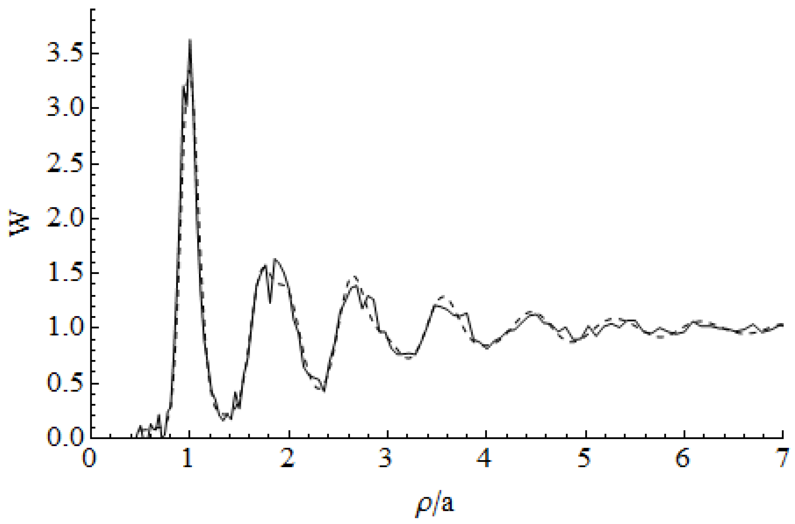
Radial distribution function of pores in porous aluminum oxide: experimental sample (solid curve) and our calculation (dashed curve).
Figure 3.
Radial distribution function of pores in porous aluminum oxide: experimental sample (solid curve) and our calculation (dashed curve).

Figure 4.
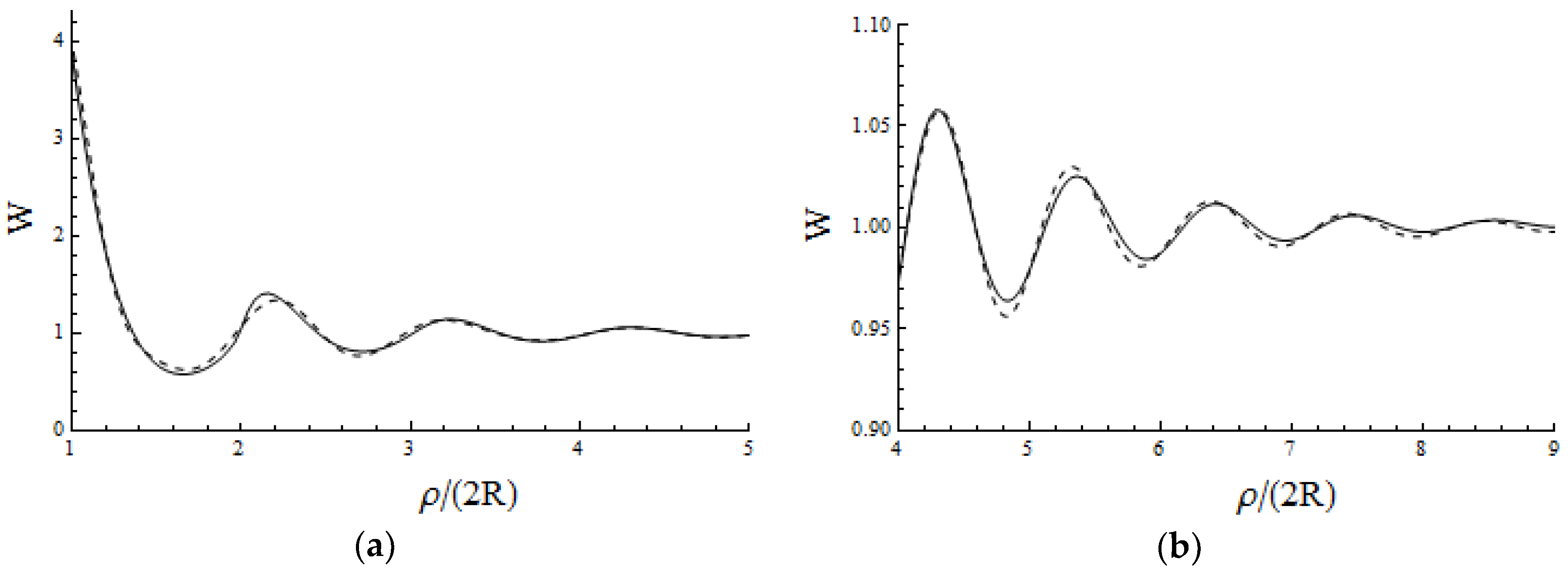
Radial distribution function for filling (a) in the range , and (b) in the range (“a tail of the distribution function”). Solid line is a solution of the Percus–Yevick equation; dashed line corresponds to the smeared lattice model.
Figure 4.
Radial distribution function for filling (a) in the range , and (b) in the range (“a tail of the distribution function”). Solid line is a solution of the Percus–Yevick equation; dashed line corresponds to the smeared lattice model.

Figure 5.
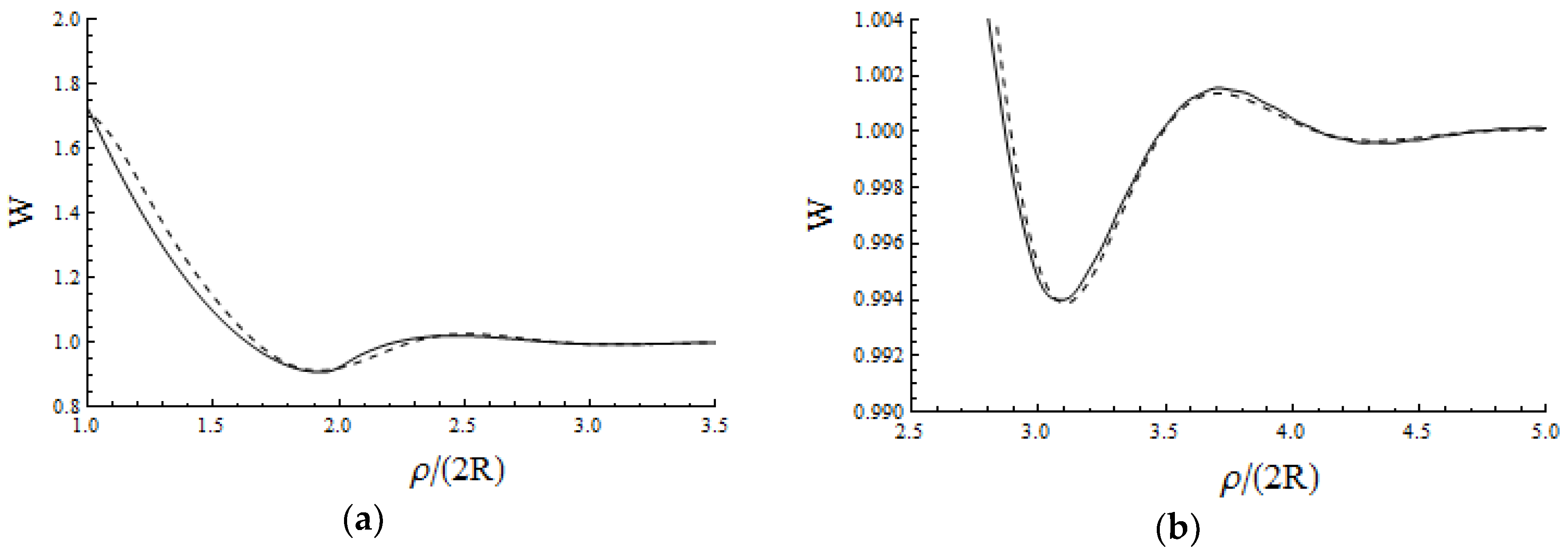
Radial distribution functions for filling (a) in the range , and (b) in the range (“a tail of the distribution function”). Solid line is a solution of the Percus–Yevick equation; dashed line corresponds to the smeared lattice model.
Figure 5.
Radial distribution functions for filling (a) in the range , and (b) in the range (“a tail of the distribution function”). Solid line is a solution of the Percus–Yevick equation; dashed line corresponds to the smeared lattice model.


Table 1.
Constants of lattices and for modeling of the radial distribution function at various packing fractions , and all the other parameters in Equations (7)–(9).
Table 1.
Constants of lattices and for modeling of the radial distribution function at various packing fractions , and all the other parameters in Equations (7)–(9).
| 0.62 | 1.04 | 1.1 | 0.158 | 0.027 | 0.4 |
| 0.6 | 1.056 | 1.12 | 0.176 | 0.03 | 0.41 |
| 0.55 | 1.095 | 1.14 | 0.192 | 0.1 | 0.45 |
| 0.5 | 1.11 | 1.2 | 0.2 | 0.2 | 0.53 |
| 0.45 | 1.112 | 1.3 | 0.209 | 0.5 | 0.7 |
| 0.4 | 1.115 | 1.6 | 0.213 | 0.9 | 1.1 |
| 0.35 | 1.117 | 2.1 | 0.224 | 1.4 | 0.75 |
| 0.3 | 1.12 | 2.3 | 0.236 | 2 | 0.6 1 |
1 All the quantities are dimensionless.
© 2018 by the authors. Licensee MDPI, Basel, Switzerland. This article is an open access article distributed under the terms and conditions of the Creative Commons Attribution (CC BY) license (http://creativecommons.org/licenses/by/4.0/).
Share and Cite
MDPI and ACS Style
Cherkas, N.L.; Cherkas, S.L. Smeared Lattice Model as a Framework for Order to Disorder Transitions in 2D Systems. Crystals 2018, 8, 290. https://doi.org/10.3390/cryst8070290
AMA Style
Cherkas NL, Cherkas SL. Smeared Lattice Model as a Framework for Order to Disorder Transitions in 2D Systems. Crystals. 2018; 8(7):290. https://doi.org/10.3390/cryst8070290
Chicago/Turabian StyleCherkas, Nadezhda L., and Sergey L. Cherkas. 2018. "Smeared Lattice Model as a Framework for Order to Disorder Transitions in 2D Systems" Crystals 8, no. 7: 290. https://doi.org/10.3390/cryst8070290
Note that from the first issue of 2016, this journal uses article numbers instead of page numbers. See further details here.