Molecular Dynamics Analysis of Synergistic Effects of Ions and Winter Flounder Antifreeze Protein Adjacent to Ice-Solution Surfaces

Abstract

The control of freezing saline water at the micrometer level has become very important in cryosurgery and cryopreservation of stem cells and foods. Adding antifreeze protein to saline water is a promising method for controlling the freezing because the protein produces a gap between the melting point and the freezing point. Furthermore, a synergistic effect of the solutes occurs in which the freezing point depression of a mixed solution is more noticeable than the sum of two freezing point depressions of single-solute solutions. However, the mechanism of this effect has not yet been clarified. Thus, we have carried out a molecular dynamics simulation on aqueous solutions of winter flounder antifreeze protein and sodium chloride or calcium chloride with an ice layer. The results show that the cations inhibit the hydrogen bond among water molecules not only in the salt solutions but also in the mixed solutions. This inhibition depends on the local number of ions and the valence of cations. The space for water molecules to form the hydrogen bonds becomes small in the case of the mixed solution of the protein and calcium chloride. These findings are consistent with the synergistic effect. In addition, it is found that the diffusion of ions near positively-charged residues is attenuated. This attenuation causes an increase in the possibility of water molecules staying near or inside the hydration shells of the ions. Furthermore, the first hydration shells of the cations become weak in the vicinity of the arginine, lysine and glutamic-acid residues. These factors can be considered to be possible mechanisms of the synergistic effect.

1. Introduction

The control of freezing water at micrometer levels has become very important in recent years in various fields: (1) cryopreservation of food and food ingredients [1,2]; (2) cryopreservation of blood, stem cells and organs to be transplanted [3]; (3) cryosurgery [4]; and (4) ice slurry for cooling or energy storage [5].

Several methods have been developed for this control of freezing. Quick freezing is a promising method to avoid the rapid growth of ice crystals and the destruction of preserved materials. However, this type of freezing requires a lot of electrical energy. Another promising method is the use of an additive, which functions to lower the freezing point while retaining the melting point. The growth of ice can be arrested by controlling the preservation temperature in a gap between these two points. Antifreeze proteins (AFPs) are appropriate additives because they produce a wide gap between the two points despite their low concentration. Furthermore, they do not increase osmotic pressure significantly and are non-toxic.

Among various AFPs discovered, HPLC6, the major fraction of winter flounder AFP, has been widely studied. HPLC6 consists of 37 amino-acid residues, and forms a helical structure [6]. Although the majority of these amino-acid residues are alanine, four threonine residues are positioned at nearly identical distances on one line parallel to the helical axis. Bi-pyramidal ice crystals, covered with ($20\overline{2}1$) pyramidal faces, are usually observed in the HPLC solution when the temperature is between the two points in a quasi-equilibrium condition. The distance between the oxygen atoms on these pyramidal faces is nearly identical to the distance between the threonine residues. Thus, it had been hypothesized that the hydrogen atoms of the threonine residues were bonded permanently to the oxygen atoms on the pyramidal faces in the ice crystal and that the water molecules were prevented from bonding to the ice surface by the Gibbs–Thomson (or Kelvin) effect [7,8]. On the other hand, Haymet et al. [9] showed by using mutants of HPLC6 that the hydrophobic interaction between the methyl group in the threonine residues and the ice surfaces plays a more important role in the ice growth inhibition mechanism than the hydrogen bond. Furthermore, Baardsnes et al. [10] suggested, from their experimental results with another mutant, that three alanine residues and an adjacent threonine residue in the central part of the HPLC6 form a surface binding to the ice. Based on these results, Davies et al. [11] and Jorov et al. [12] discussed theoretically the key role of the alanine-rich surfaces of HPLC6 in the ice-growth inhibition mechanism.

To elucidate the ice growth inhibition mechanism of HPLC6 in more detail, molecular dynamics simulations were carried out [13,14,15,16]. The simulation results showed the following scenarios: (1) there is no significant gain of hydrogen bonds of HPLC6 to the water molecules at the ice surface [13]; (2) the specific side of HPLC6, including not only the threonine residues but also the alanine residues, is oriented toward the pyramidal faces [14]; and (3) HPLC6 binds stably to the pyramidal faces when the hydrophobic residues bind to the faces [15,16]. Taken together, these results show that the van der Waals’ interactions play an important role in the binding of AFPs onto the ice surface.

Despite these results, the antifreeze mechanism due to HPLC6 in the winter flounder has not yet been fully understood. In particular, the effect of other solutes on the ice/AFP interaction has not yet been discussed in detail. Liquid, not only in winter flounder but also in food, cells, and organs, contains ions. Evans et al. [17] observed that the freezing point depression for the mixed aqueous solution of HPLC6 and sodium chloride is significantly more than the sum of the freezing point depression of the HPLC6 solution and that of salt solution (The freezing point depression of salt solutions occurs through a colligative mechanism, while this depression of AFP solutions and mixed solutions occurs through a non-colligative mechanism). This difference in the freezing point depression is due to the synergistic effect of the salt and the AFP, and is likely to be a result of the hydration shells surrounding the dissolved ions [17]. Kristiansen et al. [18] observed a similar effect for the mixed solutions of insect AFP and various salts including calcium chloride. Hagiwara and Aomatsu [19] obtained results of the depression of interface temperature in the unidirectional freezing of mixed solutions of HPLC6 and sodium chloride, which was consistent with the synergistic effects. They also discovered a decrease in the ion concentration with time at the interface of a mixed solution of HPLC6 and sodium permanganate. Hayakari and Hagiwara [20] carried out a molecular dynamics analysis on a mixed solution of HPLC6 and sodium chloride near the pyramidal face of an ice layer. They obtained the conclusion that the translational motion and freely-rotational motion of HPLC6 were attenuated by the ions as a result of the hydration of the ions. They also concluded that the approach of HPLC6 towards the ice surface with the settlement of rotation of HPLC6, caused by the hydration of ions, enhanced the interaction between a part of the protein including the threonine residues and the water molecules on the ice surface. This interaction is thought to be a possible mechanism of the synergistic effect. However, more research works, in particular molecular dynamics analysis for the mixture of AFP and other ions, are necessary for elucidating the synergistic effect.

In the present study, we carry out molecular dynamics simulations for the dilute aqueous solution of HPLC6, sodium ions, calcium ions and chloride ions near a thin ice layer covered with secondary prism or pyramidal faces, in order to analyze the interaction between the ice and AFP and the effect of ions on the interaction. The secondary prism face is the face of the ice showing the most growth [21]. Thus, the effects of solutes on the ice growth are expected to be the most noticeable. On the other hand, the pyramidal face is the face of the ice showing the least growth. Thus, the amino acid residues of HPLC6, which are bound on this face, are almost stationary. We selected the pyramidal faces only when we examined whether amino acid residues of HPLC6 influence the diffusion of the cations. It is preferable to attenuate the motion and rotation of HPLC6 for measuring the displacement and diffusion coefficient of cations.

2. Computational Procedures

We have been revising our in-house simulation program for many years [20,22,23,24,25,26]. In the present study, we have revised our program further.

2.1. Assumptions

In the main computation, we adopted the Canonical ensemble. Thus, the number of molecules, the volume of the computational domain, and the temperature were assumed to be unchanged. On the other hand, in the preliminary computation, we changed the temperature and energy to obtain the initial condition. Based on our previous study [20], we assumed that the impact of the change in the ensemble would be negligible in the period of 300 ps.

2.2. Governing Equations

The Newton–Euler equations for the translational and rotational motions of the molecules were solved at each time step, and were integrated with respect to time by using the Gear algorithm [27]. We used a 5-value Gear algorithm to the Newton equation for the translational motion, in which the time derivatives up to the fifth order were considered. We adopted a 4-value Gear algorithm to the Euler equation for the rotation. All the computations were carried out with a time step of 0.5 fs. Periodic boundary conditions were also imposed on the computational domain.

2.3. Temperature Scaling

We kept the temperature constant in a specific region for the specific period mentioned below. For this procedure, the statistical temperature, T, was defined by the total energy of the translational motion for all the molecules, K_T, and that of the rotational motion for the molecules, K_R. The temperature is written as follows:

$$T=\frac{1}{2}\left(\frac{2}{3k_{B}N}{K}_T+\frac{2}{3k_{B}N}{K}_R\right)=\frac{1}{3k_{B}N}\left(\frac{1}{2}{\displaystyle \sum _{i=1}^{N}m}{v}_i{}^2+\frac{1}{2}{\displaystyle \sum _{i=1}^N\left(I_{p{x}_i}{\omega }_{p{x}_i}{}^2+I_{p{y}_i}{\omega }_{p{y}_i}{}^2+I_{p{z}_i}{\omega }_{p{z}_i}{}^2\right)}\right),$$

(1)

where k_B is the Boltzmann constant, N is the total number of molecules, m is the mass of molecules, and I_p is the inertia moment based on its principal axis. Temperature scaling was carried out locally for certain periods in which the translational velocity, v, and the angular velocity, ω, of each molecule were changed by the following equation:

$$v_i{}^{\left(new\right)}=v_i{}^{\left(old\right)}\sqrt{\frac{T_{pd}}{T}},{\omega }_i{}^{\left(new\right)}={\omega }_i{}^{\left(old\right)}\sqrt{\frac{T_{pd}}{T}},$$

(2)

where T_pd is the predetermined temperature.

2.4. Production of Mixtures

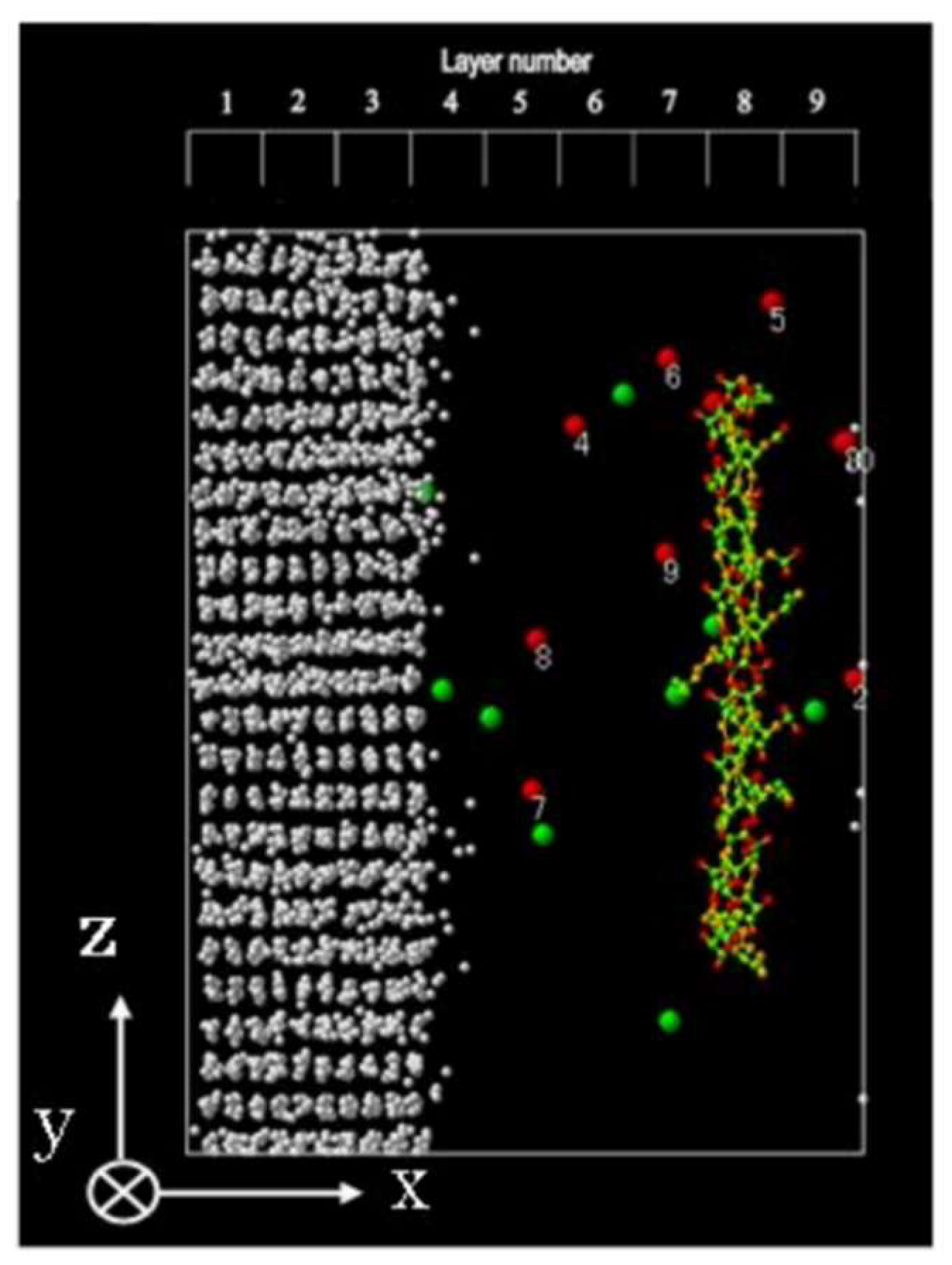
2.4.1. In the Case of Ice Layers with Prism Faces

We produced the mixture by using the following three-stage procedure in a similar way to that adopted in [26].

Stage 1: First, a small ice cube with Ih structure was formed. This procedure is the same as that described in our previous study [22]. A total of 360 water molecules were in a cubic domain of approximately 2.25 nm. In this domain, the center of mass of each molecule was allocated at the lattice of the Ih structure. The orientation of hydrogen atoms was randomly determined. Secondly, 24 ice cubes were connected to each other in order to form a large rectangular prism of ice. The dimensions of the new ice crystal were approximately 6.736 nm × 4.667 nm × 8.800 nm. The x-, y- and z-axes were located along the median, shortest, and longest edges of the rectangular prism, respectively.

Stage 2: A region of one-third in the x-direction of the rectangular prism was specified as the ice layer. The outside of the ice layer was defined as the liquid region. The computation started. The temperature for the liquid region was set at 370 K at the initial instant in order to ensure liquidization. It was decreased in steps to 250 K in a period of 350 ps (See

Table 1. Predetermined temperatures for producing the mixture of water an ice layer with prism faces.

Periods [ps]	0–50	50–100	100–150	150–200	200–250	250–300	300–350	350–
Tpd for ice [K]	10	50	100	150	200	250	260	250
Tpd for water [K]	370	370	340	310	290	280	260	250

). The restraint of the molecules in the ice was carried out at 10 K in order to reduce the impact of melting. Then, the temperature of the ice layer was increased in steps to 250 K in the period (See Table 1). The secondary prism faces were realized at the interface.

Stage 3: In the cases with the HPLC6 model, some water molecules were removed from a cocoon-shaped region in the computation result at 350 ps. The longest axes of these regions, and thus the axes of the model, were parallel to the z-axis (See Figure 1). The model was introduced into the region so that the four threonine residues of the model faced the interface at this instant.

In addition, in the cases containing the ions, a number of water molecules from the computation result at 350 ps, which were selected arbitrarily, were replaced with sodium ions, calcium ions or chloride ions. Based on our previous study [20], we assumed that the impact of the introduction of solutes would be negligible in the period of 300 ps, except for the interaction between the solutes. This exception is due to the diffusion or slow motion of ions. To simulate the NVT ensemble after 350 ps, we adopted the method developed by Nosé [28]. The computations continued until 2 ns for all the cases. This period is not too short compared with the period of 4 ns in the case of the simulation for an ice layer and water with a HPLC6 model in Ref. [15].

2.4.2. In the Cases of Ice Layers with Pyramidal Faces

We produced the mixture by using the following five-stage procedure in the same way as that developed in [20].

Stage 1: The same ice cube as that described in Section 2.4.1 was used. 60 ice cubes were connected to each other in order to form another large rectangular prism of ice.

Stage 2: Water molecules inside two regions of the triangular prisms and two regions of the pentagonal prisms were removed in order to obtain a new rectangular prism ice crystal. The two smallest surfaces of this rectangular prism were covered with the pyramidal face of ($20\overline{2}1$). The dimensions of the new ice crystal were 6.74 nm × 7.00 nm × 8.80 nm. The x-, y-, and z-axes were located along the shortest, median, and longest edges of the rectangular prism, respectively.

Stage 3: A region of approximately 32% in the y-direction of the rectangular prism was specified as the ice layer. One third of the layer in the middle of the y-direction was considered as the core of the ice layer. The outside of the ice layer was defined as the liquid region.

Stage 4: The computation started. The temperature for the liquid region was set at 370 K at the initial instant in order to ensure liquidization. It was decreased in steps to 280 K in a period of 100 ps (See

Table 2. Predetermined temperatures for producing the mixture of water an ice layer with pyramidal faces.

Periods [ps]	0–50	50–60	60–65	65–70	70–75	75–80	80–85	85–90	90–95	95–100
Tpd for ice [K]	0	0	0	0	0	50	100	150	200	250 (200)
Tpd for water [K]	370	350	330	310	290	280	280	280	280	280

). The restraint of the molecules in the ice was carried out at 0 K for the first 75 ps in order to reduce the impact of the melting. Then, the temperature for the ice layer was increased in steps for the first 95 ps and then maintained at 200 K in the core region of the ice layer and at 250 K in the surface region of the layer (See Table 2).

Stage 5: The method for introducing the protein model into the liquid water region is the same as that explained in Section 2.4.1. Consequently, the α-helical axis of HPLC6 aligned with the $\langle 10\overline{1}2\rangle$ vector of the pyramidal face. Due to the periodic boundary conditions, the distance between the adjacent protein molecules is 6.74 nm in the x-direction. This distance is wider than that of approximately 5 nm, which is the footprint of the protein/ice-surface interaction measured by Grandum et al. [29]. They measured the grooves and ridges on the ice surface with a scanning tunnel microscope. Thus, the dimension of our computational domain is sufficiently large.

A number of water molecules from the computation result at 100 ps, which were selected arbitrarily, were replaced with sodium ions, calcium ions or chloride ions in the cases containing the ions.

The method developed by Nosé was used to simulate the NVT ensemble after 100 ps. The computations continued in the period of 1 ns.

2.5. Potential Functions of Water Molecules

The TIP4P/Ice potential function proposed by Abascal et al. [30] was used for the potential function of the interaction between two water molecules. This potential was developed by the re-parameterization of the TIP4P potential [31], and has been used for ice. The TIP4P potential consists of the Coulomb potential and the Lennard–Jones potential. The numerical constants for TIP4P/Ice are almost the same as those for TIP4P except for the potential well depth of Lennard–Jones potential and the electric charges of the Coulomb potential. These parameters for TIP4P/Ice are approximately 36% and 13% higher than those of TIP4P, respectively. The Ewald summation (See Frenkel and Smit [32]) was used for the Coulomb potential in order to reduce the electrical force of distant molecules. The parameters for the Ewald summation; i.e., the width of the Gaussian distribution, the maximum value of the vector for the location of the image cell in the physical space, and the maximum value of the vector for the location of the image cell in the Fourier space—were the same as those adopted in our previous study [24].

2.6. Model of HPLC6

Table 3. Winter flounder antifreeze protein.

	Primary Structure	Molecular Weight
Winter flounder AFP	DTASDAAAAAALTAANAKAAAELTAANAAAAAAATAR	3243 Da

D: Aspartic acid, T: Threonine, S: Serine, A: Alanine, L: Leucine, N: Asparagine, K: Lysine, E: Glutamic acid, R: Arginine.

shows the primary structure of HPLC6. We adopted a rigid, helical model of HPLC6, which was similar to that used by Nada and Furukawa [15]. The location of atoms was decided based on the result obtained by Sicheri and Yang [8]. The rigidity can be considered as an overestimation of the hydrogen bond between two adjacent sites in the axial direction of the model. Flexibility can be considered by adopting an algorithm, such as SHAKE developed by Ryckaert et al. [33]. However, we did not include any algorithm for the flexibility because the time scale (or frequency) of deformation of HPLC6 due to the interaction between the model and water molecules is not clear. In addition, the fluctuation of dihedral angles of the central amino-acid residues of HPLC6 was within 9 degrees, according to the molecular dynamics simulation with AMBER by Cheng and Merz [34]. Therefore, we think that the rigid model is not too unrealistic. If we obtain results, which clearly show the validity of flexible HPLC6 models from the viewpoint of the length scale and time scale, we will show our results by using a new, flexible model in a future paper.

The OPLS parameters developed by Jorgensen et al. [35] were adopted as the potential parameters of each site of the model. The sum of the electric charges assigned to the groups in the amino-acid residues were −1. The cutoff radius was set at 1.5 nm. This is to avoid the unrealistic interaction through the ice layer between a water molecule in solution near one side of the ice layer and a water molecule in solution near the other side of the ice layer. The center of the radius was set at the indicator point of each group of sites. The parameters for the Ewald summation for the water molecules, mentioned in Section 2.5, were used also for the Coulomb potential of the sites of amino-acid residues of HPLC6 in order to reduce the electrical force between the sites and distant water molecules.

2.7. Model of Ions

The models developed by Chowdhuri and Chandra [36] were used for the sodium and chloride ions, while the model proposed by Chialvo [37] was used for the calcium ions.

2.8. Computational Conditions

The computational conditions in the present study were compared with those in the literature [13,14,15,16,20] in

Table 4. Comparison of computational conditions.

		Dalal [13]	Wierzbicki [14]	Nada [15]	Hayakari [20]	Todde [16]		Present Study
Ice Face		Pyramidal	Pyramidal	Pyramidal	Pyramidal	Prism	Pyramidal	Prism	Pyramidal
Domain size [nm3]		8.4 × 4.0 × 7.8	5.6 × 12.0 × 7.6	7.0 × 5.7 × 7.0	6.7 × 7.0 × 8.8	6.1 × 21.7 × 5.9	18.1 × 6.7 × 7.5	6.7 × 4.7 × 8.8	6.7 × 7.0 × 8.8
Ice thickness [nm]		1.4	3.8	1.4	2.3	11	9	2.3	2.3
Number of H2O molecules	liquid solid	5484 2841	11,292 5313	6520 2160	8570 4185	12,288 12288	14,724 14076	5537 1 2880	8541 2 4185
Number of AFP molecules		1	2	1	1	1	1	1	1
AFP conc. [mg/mL]		32	31	26	19	13	11	29	19
Number of cations		-	-	-	24	-	-	10	15
Ion conc. [mol/L]		-	-	-	0.15	-	-	0.10	0.10
Temperature [K]		190	165	268	260	228	228	250	250
Ensemble		NVT	NVT	NPT	NV	NPT	NPT	NVT	NVT
Potential functions		TIP3P	TIP3P	6site	TIP4P/Ice	TIP4P	TIP4P	TIP4P/Ice	TIP4P/Ice

¹ 5527 in the case of CaCl₂; ² 8526 in the case of CaCl₂.

. It is found from this table that the dimension of the liquid region and the concentration of solutes are reasonable.

3. Statistical Quantities

We discuss the following statistical quantities. These are the same as those defined in our previous studies [20,24,25,26] except for the tetrahedricity parameter.

3.1. Radial Distribution Function (RDF)

The RDF between an atom of a water molecule or an ion, and the oxygen atoms in a spherical shell is defined as follows (See, for example, Allen and Tildesley [38]):

$$g\left(r\right)=\frac{V}{4\pi r^2\Delta r{N}^2}\langle {\displaystyle \sum _i{\displaystyle \sum _{j\ne i}\delta \left(r_i-r_j\right)}}\rangle ,$$

(3)

where r=|r_i − r_j| is the distance between two atoms (or between a site and an atom), V is the volume of the computation domain, Δr is the thickness of the shell, N is the number of oxygen atoms, and δ is the delta function. Δr was equal to 0.01 nm. Please note that the total number of water molecules in the spherical domain (0 < r < ∞) was not identical because the water molecules inside the ice layer were not included in the summation in this equation.

3.2. Hydrogen Bond Correlation Function (HBCF)

In our previous study [25], we used the hydrogen-bond correlation function (hereafter abbreviated to HBCF) to analyze the hydrogen bond among water molecules. The function is defined as follows:

$$C_{HB}\left(t\right)=\frac{\langle {\displaystyle \sum _j^N{n}_{HBj}\left(t_0+t\right)n_{HBj}\left(t_0\right)}\rangle }{\langle {\displaystyle \sum _j^N{n}_{HBj}\left(t_0\right)n_{HBj}\left(t_0\right)}\rangle },$$

(4)

where n_HBj (t₀) is the number of water molecules bonded with a molecular j at a reference time t₀, and n_HBj (t₀ + t) is the number of water molecules that have maintained the hydrogen bond with a molecular j for the period of t. The cluster structure was identified by only the distance of water molecules from a specific water molecule. In the present study, we focus on water molecules in the first hydration shell of a specific ion.

3.3. Diffusion Coefficient

The diffusion coefficient can be obtained from the following equation:

$$D_S=\underset{t\to \infty }{\lim }\frac{1}{6t}\langle {\left|r_j\left(t_1+t\right)-r_j\left(t_1\right)\right|}^2\rangle ,$$

(5)

where t₁ is defined as an instant when the mean square displacement obeys the power law with time [39]. The mean square displacement, D(t), is defined by the following equation:

$$D\left(t\right)=\frac{1}{N}\langle {\displaystyle \sum _j{\left|{\mathit{r}}_j\left(t_0+t\right)-{\mathit{r}}_j\left(t_0\right)\right|}^2}\rangle ,$$

(6)

where r_j is the position vector of a molecular j, t is time, t₀ is a reference time, N is the number of molecules and the angle bracket shows a time mean value. The mean squared deviation (MSD) was obtained from the position vectors for the periods of 10 ps at an interval of 0.5 ps. The moving-averaged values of the MSD were obtained over the period of 50 ps.

3.4. Tetrahedricity Parameter

We adopted the tetrahedricity parameter [40] as an index to estimate water molecular structure in the liquid phase. The tetrahedricity parameter M_T is expressed by the following equation:

$$M_T=\frac{{\displaystyle {\sum }_{i>j}{\left(l_i-l_j\right)}^2}}{15\langle l^2\rangle }$$

(7)

where l_i are the lengths of the six edges of a tetrahedron. If the nearest four water molecules to a water molecule form a tetrahedron, M_T becomes nearly zero. On the other hand, if the distances between two of four water molecules differ from each other, M_T becomes nearly a unity. Thus, the tetrahedricity parameter shows the degree of the water structure.

4. Results and Discussion

We will discuss the results for the system of solutions with a thin ice layer covered with secondary prism faces in Section 4.1, Section 4.2, Section 4.3, Section 4.4 and Section 4.5. We will then discuss the results for the system of solutions with a thin ice layer covered with pyramidal faces in Section 4.6. The results obtained were thermodynamically non-equilibrium because the diffusion of ions and the interaction of solutes are too slow to capture their developed state.

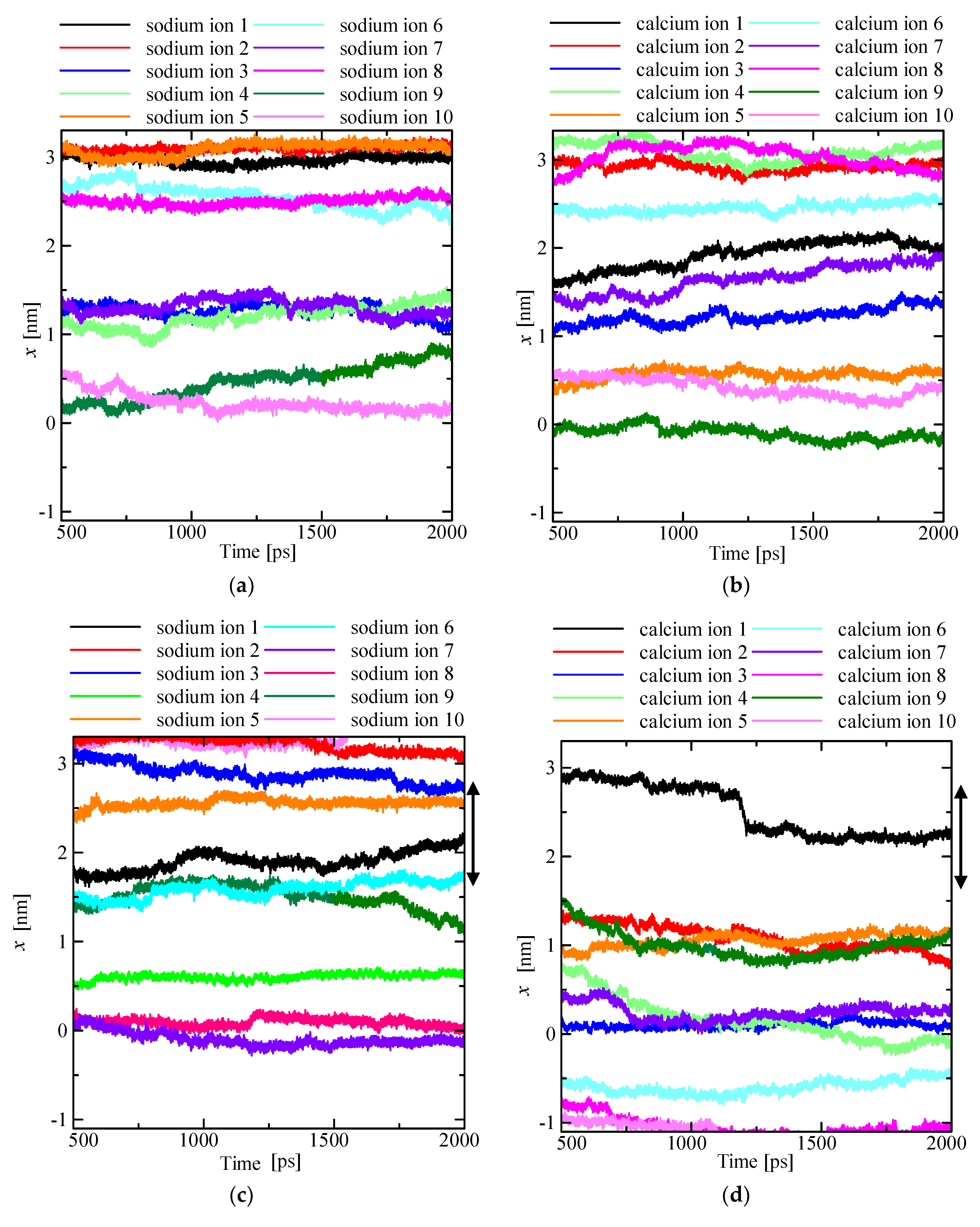
4.1. Time Changes in the Ion Positions

Figure 2 shows time changes in the ion position in the x-direction. The origin of the ordinate corresponds to the center of the computational domain. The positions close to the top and bottom edges in the graphs indicate that the corresponding ions are located close to the ice surfaces. Figure 2a,b show the time changes in the cases without HPLC6, while Figure 2c,d show the time changes in the cases with HPLC6. It is found from these figures that the changes in the ion positions were within the range of 0.5 nm for the period of 1500 ps except for one or two ions in each case. The time changes are due to the diffusion of ions or the interaction between the ions and HPLC6.

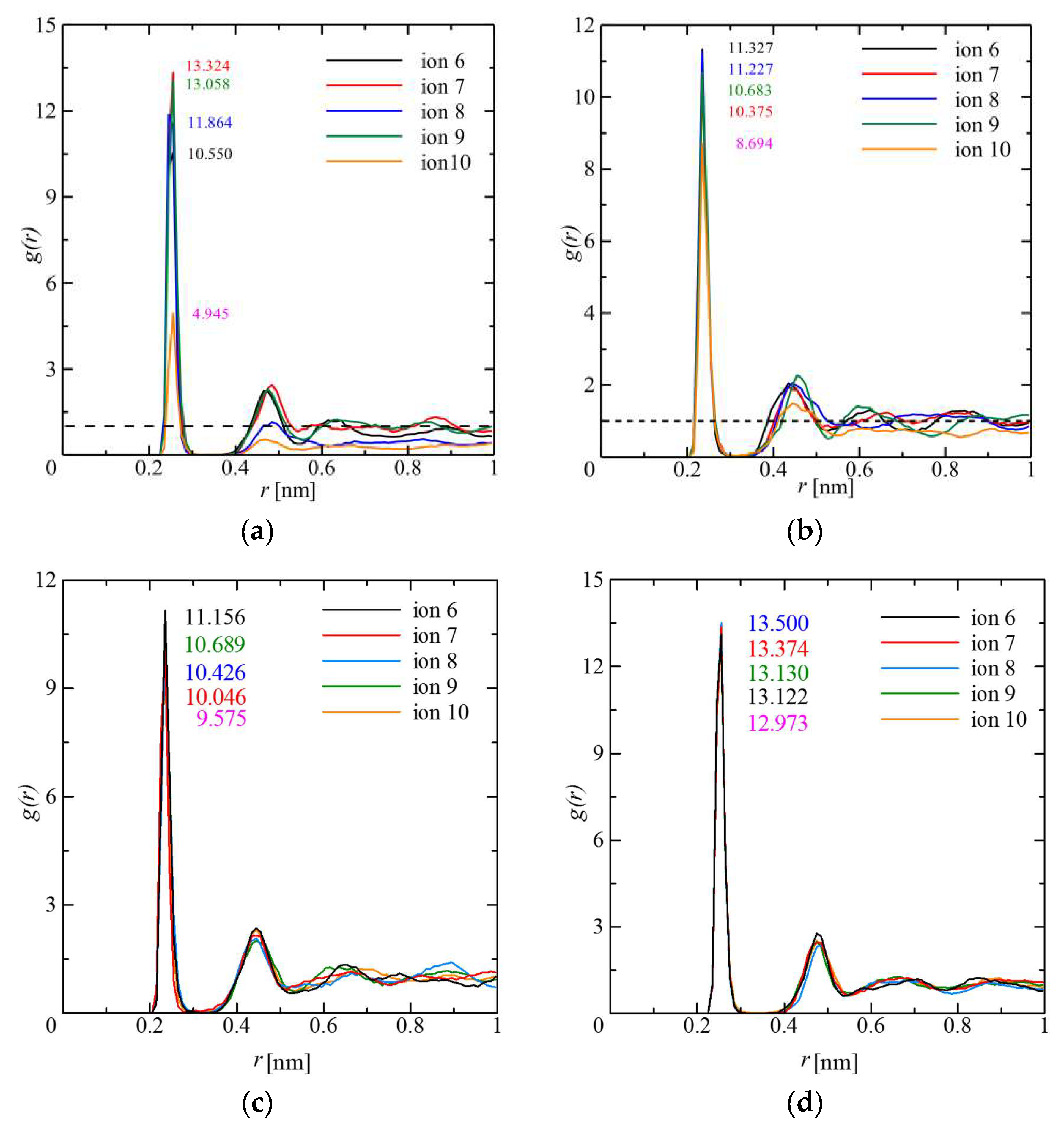
4.2. Radial Distribution Function (RDF)

Figure 3 shows typical examples of the RDF for water molecules around several ions in the mixed solutions. The peak values differ by margins of approximately 10% for the sodium ions and 45% for the calcium ions for 1500–1550 ps. On the other hand, the peak values differ by margins of approximately 4% for the sodium ions and 2% for the calcium ions for 1950–2000 ps. These changes in the differences are due to the changes in the RDFs for water molecules around the sodium ion 10, and the calcium ions 8 and 10. It is found from Figure 2c,d that these three ions gradually approached the ice surfaces by 1500 ps and that they gradually left from the locations adjacent to the ice surfaces by 2000 ps. Thus, the hydration shells of cations were not affected by the presence of HPLC6.

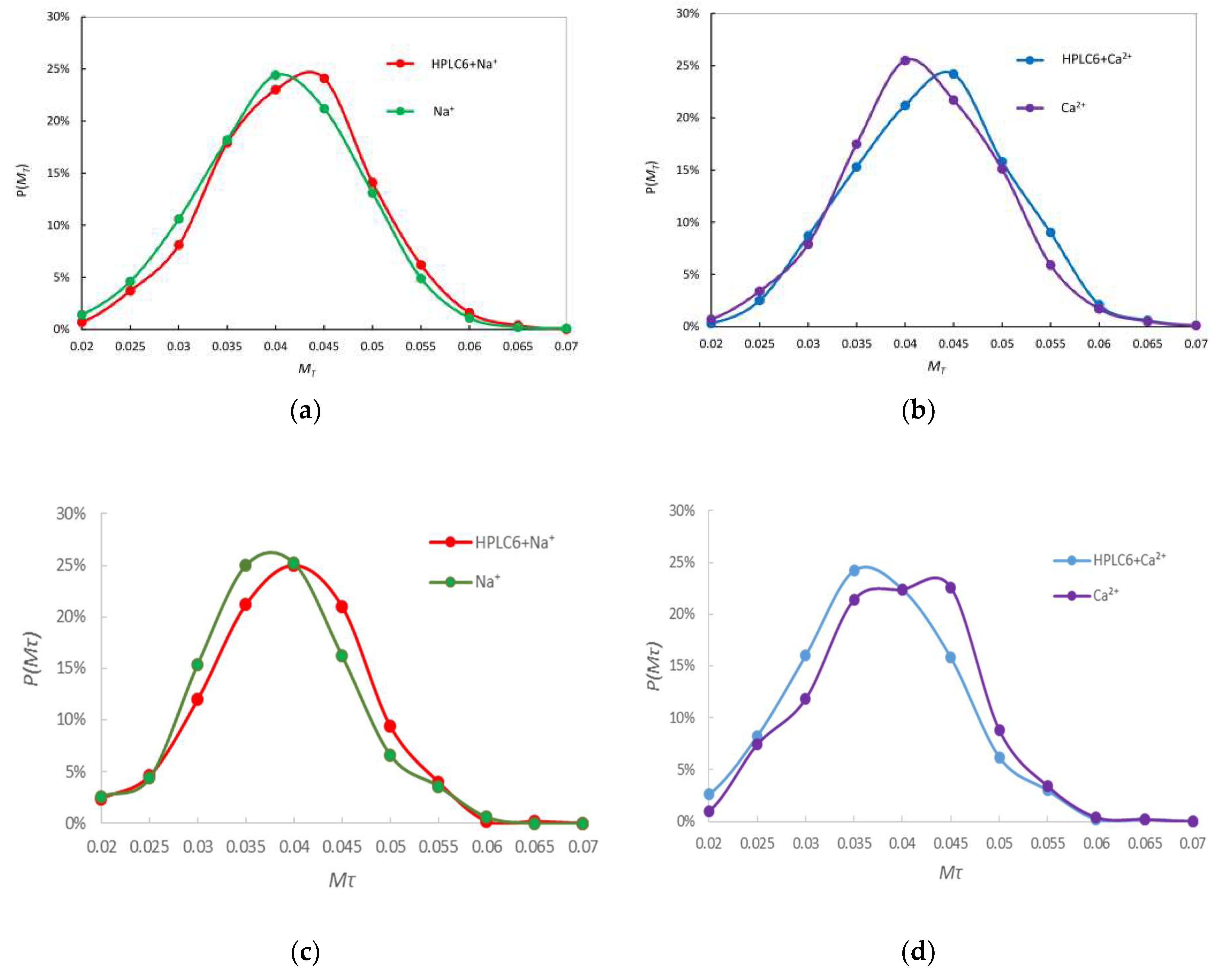
4.3. Tetrahedricity Parameter

The average value of the tetrahedricity parameter gradually decreased with time for all the solutions (See

Table 5. Average values of the tetrahedricity parameter.

Solution	NaCl	NaCl + HPLC6	CaCl2	CaCl2 + HPLC6
1000–1050 ps	0.041	0.044	0.040	0.039
1500–1550 ps	0.038	0.039	0.039	0.040
1950–2000 ps	0.038	0.039	0.039	0.037

). This shows that the tetrahedral structure of the water molecules was forming. The decreasing rate of the average values in the cases of solutions with calcium chloride was lower than that in the cases of solutions with sodium chloride. This is because the hydration shells of calcium ions, which are stronger than the hydration shells of sodium ions, disturb the tetrahedral structure.

Figure 4a,b show the probability distributions of the tetrahedricity parameter, M_T, for salt solutions and mixed solutions in the period of 1500–1550 ps. The most probable values of M_T (the values of M_T for their highest probabilities) in the case of mixed solutions are higher than those in the case of salt solutions. This indicates that the HPLC6 inhibits water molecules forming a tetrahedral structure not only near the HPLC6 itself but also far from it.

Figure 4c,d show the distributions of the tetrahedricity parameter for the salt solutions and mixed solutions in the period of 1950–2000 ps. The distribution in Figure 4c is similar to that in Figure 4a, while the distribution in Figure 4d is not similar to that in Figure 4b. This is because the time changes in the positions of the calcium ions were predominant in the mixed solution in this period (See Figure 2d).

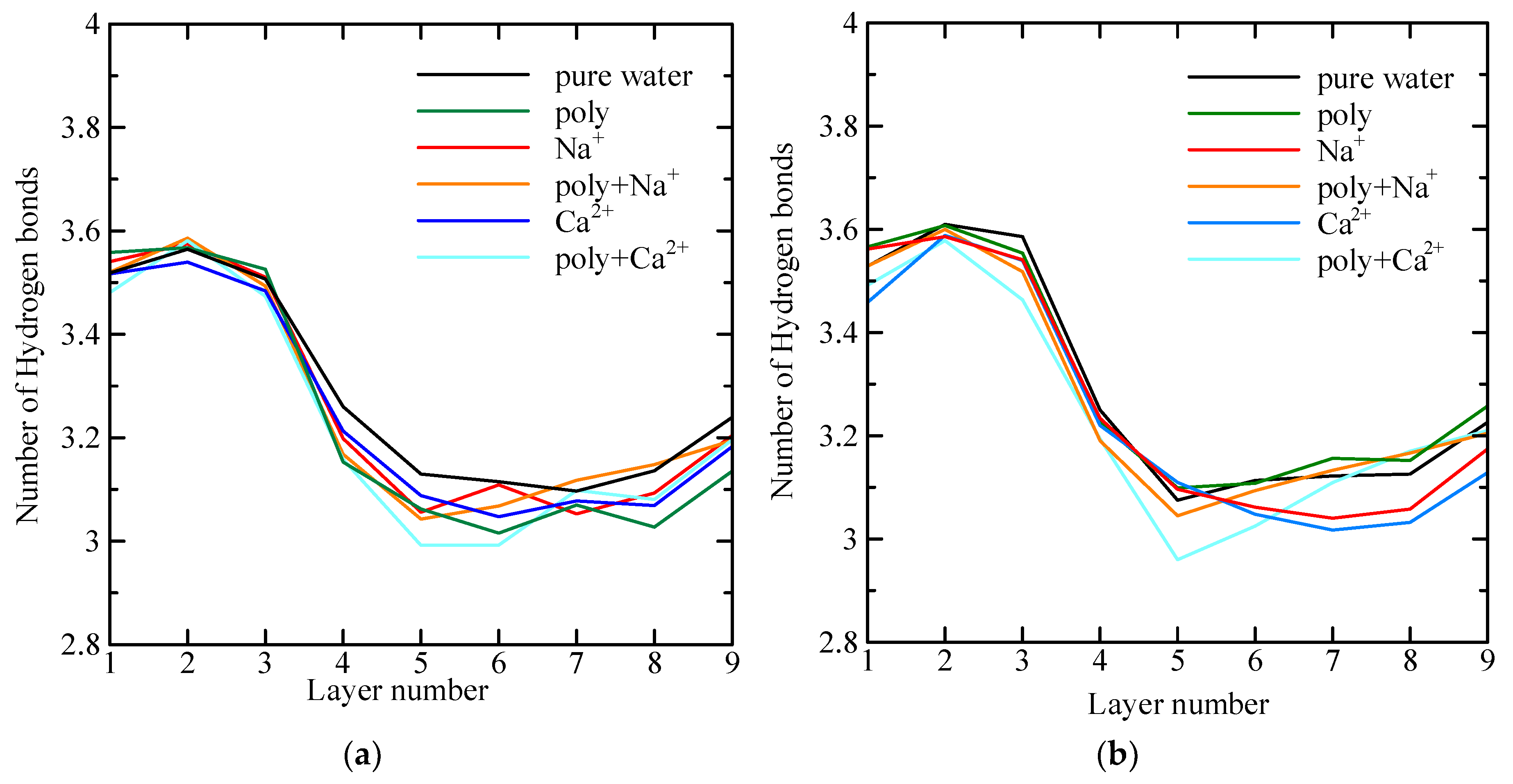
4.4. Average Number of Hydrogen Bonds

We evaluated the number of hydrogen bonds for a water molecule. The criteria for the hydrogen bond are as follows (The criterion for the angle is stricter than that proposed by Luzar and Chandler [41]):

(A)

The distance between oxygen atoms is lower than 3.5 Å.

(B)

The angle between the line connecting two oxygen atoms and the line connecting one of the two oxygen atoms and a covalent-bonded hydrogen atom is within ±15°.

We divided the computational domain into 9 layers in the x-direction, and examined the effects of ions and HPLC6 on the average number of hydrogen bonds per water molecule in each layer (See Figure 1). The thickness of each layer was 0.748 nm. In Ref. [16], the computational domain was divided into the regions of bulk ice, interface, and bulk water. The layer thickness is approximately half the interface width. Thus, the 1st, 2nd, and 3rd layers are in the bulk ice region, the 4th, 5th, 8th, and 9th layers are in the interface region, and the 6th and 7th layers are in the bulk water region.

Figure 5 shows the average number of hydrogen bonds for each layer for the periods of 1000–1050 ps and 1950–2000 ps. The first three layers were in the ice layer, while the other six layers were in the liquid region throughout the computation. Most of the residues of HPLC6 were located in the eighth layer. It is found from Figure 5a that the average numbers of hydrogen bonds for the single-solute solutions are lower than the average numbers for pure water in the layers in the liquid phase. In particular, the average number is lowest in the eighth and ninth layers for the HLPC6 solution (shown with the figure caption ‘poly’). This is the result of hydrogen bonds between water molecules and the hydrophilic residues of HPLC6. Moreover, the hydrophobic hydration due to the hydrophobic residues kept water molecules away from HPLC6.

The average number of hydrogen bonds in the 4th, 5th, and 6th layers indicates lower values for salt solutions compared with the number for pure water. (The salt solutions are shown with the figure caption ‘Na⁺’ and ‘Ca²⁺’. Note that the anion Cl⁻ also contributed.) This is because water molecules are more attracted by the hydration shells of ions, particularly the cations in these layers. The number of hydrogen bonds decreased more than 4% in the 5th and 6th layers of the mixed solution of HPLC6 and CaCl₂ compared with the number of bonds in pure water, although the concentration of HPLC6 and CaCl₂ was 8.9 mM and 0.1 M, respectively. The number of calcium ions in the 5th layers increased from 1 (ion no. 3 in Figure 2d) to 3 (ion no. 3, 4 and 7) during the period 700–800 ps in the mixed solution. It can be surmised that the strong hydration shells of calcium ions prevent water molecules from forming the hydrogen bonds in these two layers.

In Figure 5b, the number of hydrogen bonds of salt solutions in the 7th and 8th layers is lower than that in the other cases in the period of 1950–2000 ps. This is because the time changes in the positions of some sodium ions (3 and 6 in Figure 2a) and calcium ions (1 and 7 in Figure 2b) in these layers are more noticeable than the time changes in the positions of the other ions.

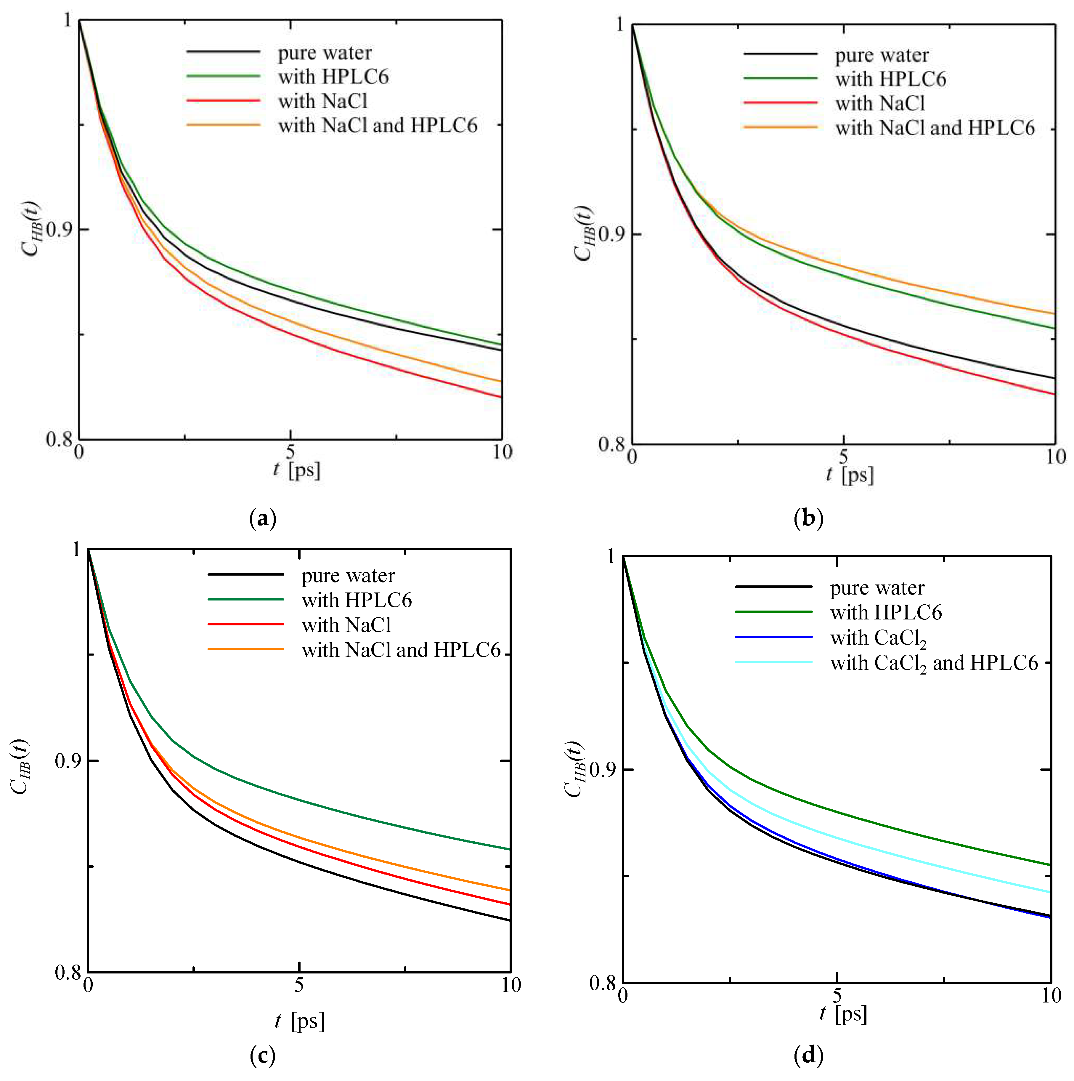
4.5. Hydrogen Bond Correlation Function (HBCF)

Figure 6 shows the hydrogen bond correlation function (HBCF) as a function of time for the fifth and eighth layers. It is found from Figure 6a that the HBCF for the 5th layer of the NaCl solution and mixed solution indicates lower values than that for the pure water and HPLC6 solution at any time in the period of 1000–1050 ps. This indicates that the hydrogen bond among water molecules was disturbed by the ions and their motion in the 5th layer. A similar result was obtained for the CaCl₂ solution [37].

It is found from Figure 6b that the HBCF for the eighth layer of the HPLC6 solution and mixed solution indicates higher values than that for the pure water and NaCl solution at any time in the period of 1000–1050 ps. This clearly indicates that the hydrogen bond among water molecules near the HPLC6 was enhanced by the HPLC6 molecule in the 8th layer. This may result in the formation of hydrophobic hydration shells around the alanine residues of HPLC6 in this layer. The effect of ions on the hydrogen bonding is not noticeable in this layer in this period probably because the hydration shells around the ions have not yet been formed well.

Figure 6c shows the HBCF of the solutions for the 5th layer in the period of 1950–2000 ps. The difference between the correlation function in the case of the HPLC6 solution and that in the other cases became noticeable compared with the difference shown in Figure 4a. This is probably because the space for forming the hydrogen bond among water molecules became small as a result of the growth of hydrophobic hydration shells around the HPLC6.

Figure 6d shows the HBCF of the solutions with CaCl₂ for the 8th layer in the period of 1000–1050 ps. The calcium ions in this layer did not disturb the hydrogen bond in the case of the salt solution. This is because only one calcium ion (6 in Figure 2b) was in this layer in this period. On the other hand, the ions in the case of the mixed solution disturbed the hydrogen bond in the layer in the period. This is probably because the effect of one calcium ion (1 in Figure 2d) in the 9th layer, which approached and entered into the 8th layer just after the period, was remarkable. This is consistent with the synergistic effects of ions and HPLC6.

4.6. Interaction between Cations and Amino Acid Residues

4.6.1. Surface-Bound Water Molecules

We allocated the HPLC6 model so that the four threonine residues were closest to the pyramidal face. Also, three alanine residues (the 6th, 17th and 28th) were close to the face. Thus, the spatial arrangement of HPLC6 was similar to that in Ref. [15].

We monitored the motion of many water molecules between the atom groups of the threonine residues and the ice surface. We discovered that at least three water molecules were nearly stationary, while the other water molecules nearby moved more rapidly in three locations; (1) near the hydroxyl group of the 24th threonine residue; (2) near the methyl group of the threonine residue; and (3) near the hydroxyl group of the 35th threonine residue. We believe that these nearly stationary water molecules are surface-bound water molecules.

4.6.2. Diffusion Coefficient

Table 6. Ratio of diffusion coefficients of cations to the diffusion coefficient of water.

Na+			Ca2+
Near Arginine	Nohara	Baştuğ	Near Lysine	Near Glutamic Acid	Nohara	Baştuğ
0.18	0.46	0.42	0.19	1.06	0.28	0.31

shows the ratios of the diffusion coefficient of a cation nearest to a specific amino-acid residue to the diffusion coefficient of water. The arginine, lysine and glutamic-acid residues are located opposite to the four threonine residues with respect to the HPLC6 axis. Thus, these residues were inside the water region because the four threonine residues faced the interface.

This table also shows the ratios obtained by Nohara and Hagiwara [26] and Baştuğ and Kuyucak [42]. Ref. [26] dealt with the ions in supercooled water between ice layers with the prism faces, and used approximately one-third of the number of water molecules. Ref. [42] dealt with the ions in water at 273 K without any ice, and used a different potential function for water and ions.

It is found from this table that the ratio for the sodium ion near the arginine residue (R in Table 3) is much lower than the ratio in [26,42]. This shows that the diffusion of the sodium ion in the vicinity of the arginine residue was attenuated. This is probably a result of electrostatic attraction between the oxygen atoms of water molecules in the hydration shell of the sodium ion and the C = NH group of the arginine residue because this group is positively electrified in water and the oxygen atoms are negatively electrified. Similarly, the ratio for the calcium ion near the lysine residue (K in Table 3) is lower than the ratio in [26,42]. The attenuation of diffusion of the calcium ion in the vicinity of the lysine residue is probably a result of electrostatic attraction between the oxygen atoms of water molecules in the hydration shells of the calcium ion and the amino group of the lysine residue. This is because this amino group is also positively electrified in water. On the other hand, the ratio for the calcium ion near the glutamic acid residue (E in Table 3) is much higher than the ratio in [26,42]. This shows that the diffusion of the calcium ion in the vicinity of the glutamic acid residue was enhanced. This is probably a result of electrostatic repulsion between the oxygen atoms of water molecules in the hydration shells of the calcium ion and the carboxyl group of the glutamic acid residue because the carboxyl group is negatively electrified in water. The side chains of all the other residues of HPLC6 except for the aspartic acid residue are neutrally electrified. It can be concluded that the diffusion of cations in the vicinity of HPLC6 depends on the electrified amino acid residues of HPLC6.

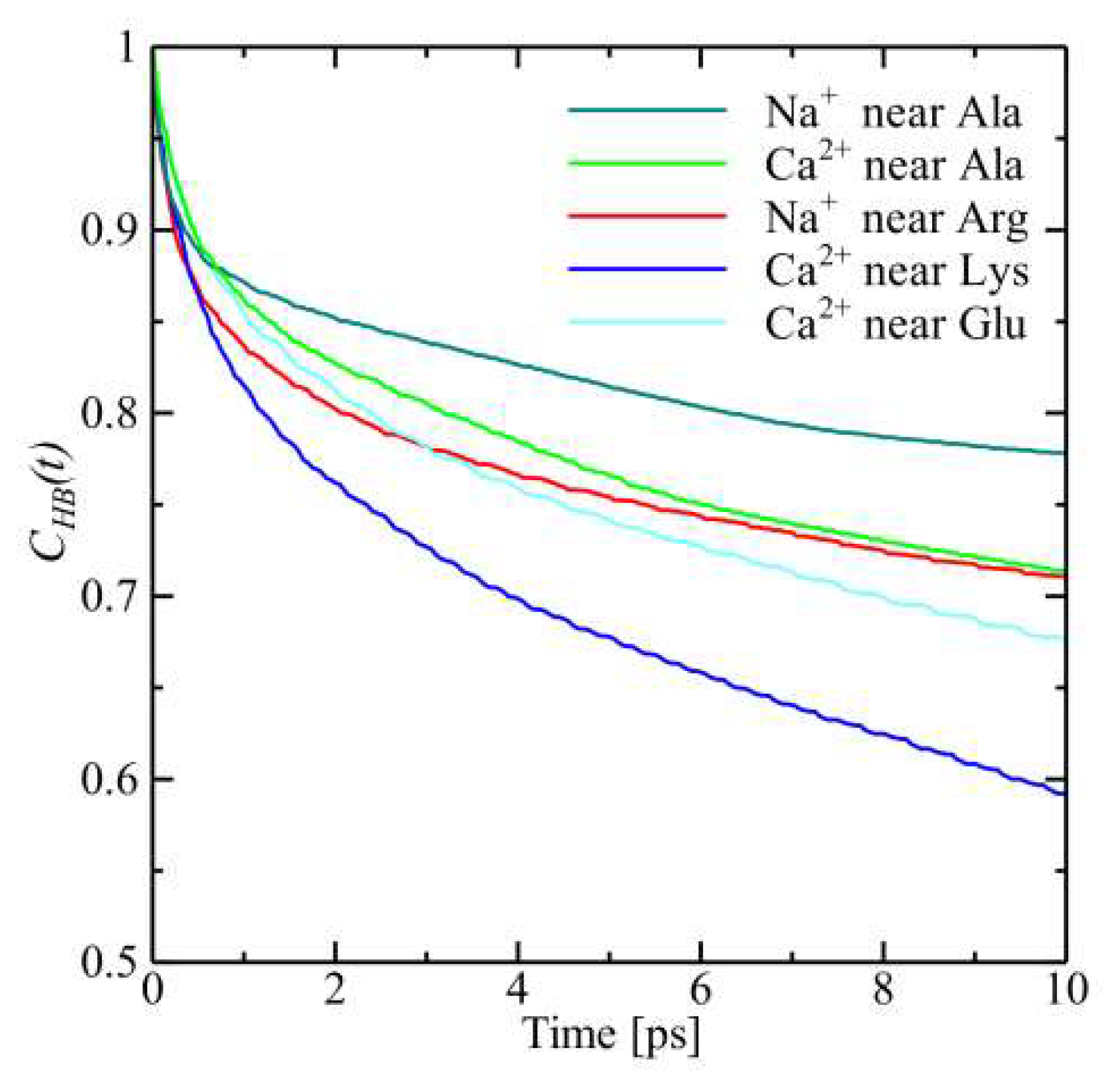
4.6.3. Hydrogen Bond Correlation Function (HBCF)

Figure 7 shows the hydrogen bond correlation function (HBCF) as a function of time for water molecules in the first hydration shell of the cations in the vicinity of the specific amino acid residues. The HBCF decreases with an increase in time. To discuss the robustness of the hydration shell of the cations, we compare the values of the HBCF at 10 ps. It is found from this figure and Figure 6 that the values for the cations near the electrified residues are lower than those for the cations near alanine residues and the values of water molecules in Figure 6. This shows that the first hydration shell of the cations in the vicinity of the electrified residues does not become robust and the water molecules in the first hydration shell can easily leave the shell. This weakening of the hydration shell of the cations enhances the motions of ions and water molecules. The motion enhancement of ions and water molecules can cause the attenuation of the incorporation of water molecules into the ice lattice at the interface. Also, the enhancement of ion motion is consistent with the decrease in the ion concentration of the mixed solution [19] described in the Introduction. Thus, the motion enhancement of ions and water molecules is a reason for the synergistic effect.

The higher values of HBCF for the cations near alanine residues show that the first hydration shells of the cations in the vicinity of these residues remain robust. The robustness of the hydrophobic hydration shells around these residues is also expected. These robust shells also contribute to the synergistic effect. The discussion in this section is therefore consistent with the discussion in Section 4.4.

5. Conclusions

A molecular dynamics simulation was carried out on a mixture of water, a model of HPLC6 (winter flounder antifreeze protein), sodium ions, calcium ions, chloride ions and a thin ice layer. The main conclusions obtained are the following:

(1). The hydrogen bond among water molecules is inhibited by the cations even in the case of the mixed solutions. This is due to the hydration shells of the moving ions. This inhibition is more noticeable with an increase in the number density of ions and the valence of cations.

(2). The effective space for water molecules to form the hydrogen bonds becomes smaller in a region far from the HPLC6 as a result of the hydration shells of calcium ions in this region. This is also consistent with the synergistic effect of the mixed solutions of HPLC6 and CaCl₂.

(3). The negatively or positively electrified residues of HPLC6 respectively enhance or attenuate the diffusion of the cations in water.

(4). The hydrophobic hydration shells around the alanine residues of HPLC6 remain robust, as does the first hydration shells of the cations in the vicinity of these residues. On the other hand, the first hydration shells of the cations in the vicinity of the electrified residues do not become robust. The weakening of the hydration shells of the cations enhances the motions of ions and water molecules. The motion enhancement of ions and water molecules can cause the attenuation of the incorporation of water molecules into the ice lattice at the interface.

(5). The inhibition of the hydrogen bond due to the hydration shells of the moving ions in conclusion (1) and the weakening of the hydration shells of cations as a result of the electrified amino-acid residues nearby in conclusion (4) are the possible mechanisms of the synergistic effects suggested by Evans et al. [17].

References

1. Ustun, N.S.; Turhan, S. Antifreeze proteins: Characteristics, function, mechanism of action, sources and application to foods. J. Food Process. Preserv. 2015, 39, 3189–3197. [Google Scholar] [CrossRef]
2. Li, B.; Sun, D.-W. Novel methods for rapid freezing and thawing of foods—A review. J. Food Eng. 2002, 54, 175–182. [Google Scholar] [CrossRef]
3. Amir, G.; Rubinsky, B.; Basheer, S.Y.; Horowitz, L.; Jonathan, L.; Feinberg, M.S.; Smolinsky, A.K.; Lavee, L. Improved viability and reduced apoptosis in sub-zero 21-hour preservation of transplanted rat hearts using anti-freeze proteins. J. Heart Lung Transpl. 2005, 24, 1915–1929. [Google Scholar] [CrossRef] [PubMed]
4. Shitzer, A. Cryosurgery: Analysis and experimentation of cryoprobes in phase changing media. J. Heat Transf. 2011, 133. [Google Scholar] [CrossRef]
5. Grandum, S.; Yabe, A.; Tanaka, M.; Takemura, F.; Nakagomi, K. Characteristics of ice slurry containing antifreeze protein for ice storage applications. J. Thermophys. Heat Transf. 1997, 11, 461–466. [Google Scholar] [CrossRef]
6. Yang, D.S.C.; Sax, M.; Chakrabatty, A.; Hew, C.L. Crystal structure of an antifreeze polypeptide and its mechanistic implications. Nature 1988, 333, 232–237. [Google Scholar] [CrossRef] [PubMed]
7. Chao, H.; Houston, M.E., Jr.; Hodges, R.S.; Kay, C.M.; Sykes, B.D.; Loewen, M.C.; Davies, P.L.; Sönnichsen, F.D. A diminished role for hydrogen bonds in antifreeze protein binding to ice. Biochemistry 1997, 36, 14652–14660. [Google Scholar] [CrossRef] [PubMed]
8. Sicheri, F.; Yang, D.S.C. Ice-binding structure and mechanism of an antifreeze protein from winter flounder. Nature 1995, 375, 427–431. [Google Scholar] [CrossRef] [PubMed] [Green Version]
9. Haymet, A.D.J.; Ward, L.G.; Harding, M.M. Winter flounder “antifreeze” proteins: Synthesis and ice growth inhibition of analogues that probe the relative importance of hydrophobic and hydrogen-bonding interactions. J. Am. Chem. Soc. 1999, 121, 941–948. [Google Scholar] [CrossRef]
10. Baardsnes, J.; Kondejewski, L.H.; Hodges, R.S.; Chao, H.; Kay, C.; Davies, P.L. New ice-binding face for type I antifreeze protein. FEBS Lett. 1999, 463, 87–91. [Google Scholar] [CrossRef] [Green Version]
11. Davies, P.L.; Baardsnes, J.; Kuiper, M.J.; Walker, V.K. Structure and function of antifreeze proteins. Philos. Trans. R. Soc. Lond. B 2002, 357, 927–935. [Google Scholar] [CrossRef] [PubMed] [Green Version]
12. Jorov, A.; Zhorov, B.S.; Yang, D.S.C. Theoretical study of interaction of winter flounder antifreeze protein with ice. Protein Sci. 2004, 13, 1524–1537. [Google Scholar] [CrossRef] [PubMed] [Green Version]
13. Dalal, P.; Knickelbein, J.; Haymet, A.D.J.; Sönnichsen, F.D.; Madura, J. Hydrogen bond analysis of type 1 antifreeze protein in water and the ice/water interface. PhysChemComm 2001, 4, 32–36. [Google Scholar] [CrossRef]
14. Wierzbicki, A.; Dalal, P.; Cheatham, T.E., III; Knickelbein, J.E.; Haymet, A.D.J.; Madura, J.D. Antifreeze proteins at the ice/water interface: Three calculated discriminating properties for orientation of type I proteins. Biophys. J. 2007, 93, 1442–1451. [Google Scholar] [CrossRef] [PubMed]
15. Nada, H.; Furukawa, Y. Growth inhibition mechanism of an ice-water interface by a mutant of winter flounder antifreeze protein: A molecular dynamics study. J. Phys. Chem. B 2008, 112, 7111–7119. [Google Scholar] [CrossRef] [PubMed]
16. Todde, G.; Hovmöller, S.; Laaksonen, A. Influence of antifreeze proteins on the ice/water interface. J. Phys. Chem. B 2015, 119, 3407–3413. [Google Scholar] [CrossRef] [PubMed]
17. Evans, R.P.; Hobbs, R.S.; Goddard, S.V.; Fletcher, G.L. The importance of dissolved salts to the in vivo efficacy of antifreeze proteins. Comp. Biochem. Physiol. Part A 2007, 148, 556–561. [Google Scholar] [CrossRef] [PubMed]
18. Kristiansen, E.; Pedersen, S.A.; Zachariassen, K.E. Salt-induced enhancement of antifreeze protein activity: A salting-out effect. Cryobiology 2008, 57, 122–129. [Google Scholar] [CrossRef] [PubMed]
19. Hagiwara, Y.; Aomatsu, H. Supercooling enhancement by adding antifreeze protein and ions to water in a narrow space. Int. J. Heat Mass Transf. 2015, 86, 55–64. [Google Scholar] [CrossRef]
20. Hayakari, K.; Hagiwara, Y. Effects of ions on winter flounder antifreeze protein and water molecules near an ice/water interface. Mol. Simul. 2012, 38, 26–37. [Google Scholar] [CrossRef]
21. Nada, H.; Furukawa, Y. Anisotropy in growth kinetics at interfaces between proton-disordered hexagonal ice and water: A molecular dynamics study using the six-site model of H2O. J. Cryst. Growth 2005, 283, 242–256. [Google Scholar] [CrossRef]
22. Yokoyama, T.; Hagiwara, Y. Molecular dynamics simulation for the mixture of water and an ice nucleus. Mol. Simul. 2003, 29, 235–248. [Google Scholar] [CrossRef]
23. Iwasaki, K.; Hagiwara, Y. Inhibition of ice nucleus growth in water by alanine dipeptide. Mol. Simul. 2004, 30, 487–500. [Google Scholar] [CrossRef]
24. Nobekawa, T.; Taniguchi, H.; Hagiwara, Y. Interaction between a twelve-residue segment of antifreeze protein type I, or its mutants, and water molecules. Mol. Simul. 2008, 34, 309–325. [Google Scholar] [CrossRef]
25. Nobekawa, T.; Hagiwara, Y. Interaction among the twelve-residue segment of antifreeze protein type I, or its mutants, water and a hexagonal ice crystal. Mol. Simul. 2008, 34, 591–610. [Google Scholar] [CrossRef]
26. Nohara, Y.; Hagiwara, Y. Diffusion of cations in salt solutions between ice walls. Mol. Simul. 2015, 41, 980–985. [Google Scholar] [CrossRef]
27. Gear, C.W. Numerical Initial Value Problems in Ordinary Differential Equations; Prentice-Hall: Upper Saddle River, NJ, USA, 1971. [Google Scholar]
28. Nosé, S. A molecular dynamics method for simulations in the canonical ensemble. Mol. Phys. 1984, 52, 255–268. [Google Scholar] [CrossRef]
29. Grandum, S.; Yabe, A.; Nakagomi, K.; Tanaka, M.; Takemura, F.; Kobayashi, Y.; Frivik, P.-E. Analysis of ice crystal growth for a crystal surface containing adsorbed antifreeze proteins. J. Cryst. Growth 1999, 205, 382–390. [Google Scholar] [CrossRef]
30. Abascal, J.L.F.; Sanz, E.; Fernández, R.G.; Vega, C. A potential model for the study of ices and amorphous water: TIP4P/Ice. J. Chem. Phys. 2005, 122. [Google Scholar] [CrossRef] [PubMed]
31. Jorgensen, W.J.; Chandrasekhar, J.; Madura, J.D.; Impey, R.W.; Klein, M.L. Comparison of simple potential functions for simulating liquid water. J. Chem. Phys. 1983, 79, 926–935. [Google Scholar] [CrossRef]
32. Frenkel, D.; Smit, B. Understanding Molecular Simulation; Academic Press: San Diego, CA, USA, 1996. [Google Scholar]
33. Ryckaert, J.P.; Ciccotti, G.; Berendsen, H.J.C. Numerical integration of the Cartesian equations of motion of a system with constraints: Molecular dynamics of n-alkanes. J. Comput. Phys. 1977, 23, 327–341. [Google Scholar] [CrossRef]
34. Cheng, A.; Merz, K.M., Jr. Ice-binding mechanism of winter flounder antifreeze proteins. Biophys. J. 1997, 73, 2851–2873. [Google Scholar] [CrossRef] [Green Version]
35. Jorgensen, W.L.; Tirado-Rives, J. The OPLS potential functions for proteins: Energy minimizations for crystals of cyclic peptides and crambin. J. Am. Chem. Soc. 1988, 110, 1657–1666. [Google Scholar] [CrossRef] [PubMed]
36. Chowdhuri, S.; Chandra, A. Molecular dynamics simulations of aqueous NaCl and KCl solutions: Effects of ion concentration on the single-particle pair, and collective dynamical properties of ions and water molecules. J. Chem. Phys. 2001, 115, 3732–3741. [Google Scholar] [CrossRef]
37. Chialvo, A.A. The structure of CaCl2 aqueous solutions over a wide range of concentration. Interpretation of diffraction experiments via molecular simulation. J. Chem. Phys. 2003, 119, 8052–8061. [Google Scholar] [CrossRef]
38. Allen, M.P.; Tildesley, D.J. Computer Simulation of Liquid; Oxford Science: Oxford, UK, 1987. [Google Scholar]
39. Habasaki, J.; Ngai, K.L. Heterogeneous dynamics of ionic liquids from molecular dynamics simulations. J. Chem. Phys. 2008, 129, 194501. [Google Scholar] [CrossRef] [PubMed]
40. Holzmann, J.; Ludwig, R.; Geiger, A.; Paschek, D. Pressure and salt effects in simulated water: Two sides of the same coin? Angew. Chem. Int. Ed. 2007, 46, 8907–8911. [Google Scholar] [CrossRef] [PubMed]
41. Luzar, A.; Chandler, D. Hydrogen-bond kinetics in liquid water. Nature 1996, 379, 55–57. [Google Scholar] [CrossRef]
42. Baştuğ, T.; Kuyucak, S. Temperature dependence of the transport coefficients of ions from molecular dynamics simulations. Chem. Phys. Lett. 2005, 408, 84–88. [Google Scholar] [CrossRef]
Figure 1. The computational domain with an ice layer with prism faces. White dots show oxygen atoms of water molecules in the bulk ice region (water molecules in the liquid region are not shown). Red dots and green dots show sodium ions and chloride ions, respectively. Many dots connected show the HPLC6 model. Nine layers are defined in the computational domain.
Crystals 08 00302 g001
Figure 2. Time changes in the positions of ions; (a) Sodium ions in the NaCl solution, (b) Calcium ions in the CaCl2 solution, (c) Sodium ions in the mixed solution, (d) Calcium ions in the mixed solution. The ice layer was located in the range of −3.366 < x < −1.123 [nm] during the period. The arrows in (c) and (d) show the range of location of HPLC6 during the period.
Crystals 08 00302 g002
Figure 3. Radial distribution functions of water molecules around cations; (a) Sodium ions for 1500–1550 ps, (b) Calcium ions for 1500–1550 ps, (c) Sodium ions for 1950–2000 ps, (d) Calcium ions for 1950–2000 ps.
Crystals 08 00302 g003
Figure 4. Distributions of the tetrahedricity parameter; (a) in the case with NaCl for 1500–1550 ps, (b) in the case with CaCl2 for 1500–1550 ps, (c) in the case with NaCl for 1950–2000 ps, (d) in the case with CaCl2 for 1950–2000 ps.
Crystals 08 00302 g004
Figure 5. Number of hydrogen bonds in the layers; (a) for 1000–1050 ps, (b) for 1950–2000 ps.
Crystals 08 00302 g005
Figure 6. Hydrogen bond correlation functions in two layers; (a) 5th layer for 1000–1050 ps, (b) 8th layer for 1000–1050 ps, (c) 5th layer for 1950–2000 ps, (d) 8th layer for 1000–1050 ps.
Crystals 08 00302 g006
Figure 7. Hydrogen bond correlation functions of the cations.
Crystals 08 00302 g007