
Statistical and Dynamical Properties of Topological Polymers with Graphs and Ring Polymers with Knots

Department of Physics, Faculty of Core Research, Ochanomizu University, Ohtsuka 2-1-1, Bunkyo-ku, Tokyo 112-8610, Japan
*
Author to whom correspondence should be addressed.
Polymers 2017, 9(7), 252; https://doi.org/10.3390/polym9070252
Submission received: 26 January 2017
/
Revised: 22 June 2017
/
Accepted: 23 June 2017
/
Published: 28 June 2017
(This article belongs to the Special Issue Semiflexible Polymers)
Abstract
:We review recent theoretical studies on the statistical and dynamical properties of polymers with nontrivial structures in chemical connectivity and those of polymers with a nontrivial topology, such as knotted ring polymers in solution. We call polymers with nontrivial structures in chemical connectivity expressed by graphs “topological polymers”. Graphs with no loop have only trivial topology, while graphs with loops such as multiple-rings may have nontrivial topology of spatial graphs as embeddings in three dimensions, e.g., knots or links in some loops. We thus call also such polymers with nontrivial topology “topological polymers”, for simplicity. For various polymers with different structures in chemical connectivity, we numerically evaluate the mean-square radius of gyration and the hydrodynamic radius systematically through simulation. We evaluate the ratio of the gyration radius to the hydrodynamic radius, which we expect to be universal from the viewpoint of the renormalization group. Furthermore, we show that the short-distance intrachain correlation is much enhanced for real topological polymers (the Kremer–Grest model) expressed with complex graphs. We then address topological properties of ring polymers in solution. We define the knotting probability of a knot K by the probability that a given random polygon or self-avoiding polygon of N vertices has the knot K. We show a formula for expressing it as a function of the number of segments N, which gives good fitted curves to the data of the knotting probability versus N. We show numerically that the average size of self-avoiding polygons with a fixed knot can be much larger than that of no topological constraint if the excluded volume is small. We call it “topological swelling”.
1. Introduction
1.1. Topological Polymers and Knotted Ring Polymers
Polymers of novel knotted structures and those of complex chemical connectivity expressed by graphs have been found in various fields recently, such as those of DNA, proteins and synthetic polymers [1,2,3,4,5,6,7,8]. Statistical and dynamical properties of polymers with nontrivial structures in chemical connectivity and those derived from topological constraints such as ring polymers with fixed knots have attracted much interest in several branches of physics, chemistry and biology. Although some properties of ring polymers in solution were studied rather early, such as in the 1940s and 1960s [9,10,11,12], circular DNA had been found in nature in the 1960s, and knotted DNA molecules are synthesized in experiments in the 1980s [2,13,14,15]; looped or knotted proteins had been found in nature during the 2000s [5,16]. Here, we recall that the three-dimensional conformation of a ring polymer in solution is described by a closed curve with no ends, and its topology is represented by a knot. Several theoretical studies on knotted ring polymers in solution are reviewed in [3,4].
After novel developments in synthetic chemistry, polymers with various different chemical or topological structures were synthesized in experiments recently during the last decade such as ring polymers, tadpole (or lasso) polymers, double-ring (or di-cyclic) polymers, multiple-ring (or multi-cyclic) polymers and even complete bipartite graph polymers [8,17,18,19,20,21,22,23,24,25]. In Figure 1, some graphs corresponding to simple topological polymers are shown. Lasso polymers are studied in association with protein folding [26]. For multiple-ring (or multi-cyclic) polymers, hydrodynamic properties were theoretically studied by a perturbative method in the 1960s [27]. For double-ring polymers, they are studied by the Monte Carlo (MC) simulation of self-avoiding double-polygons [28]. It seems that topological polymers are also related to ravels as novel entanglements of spatial graphs [29] and non-planar RNA structures corresponding to pseudoknots [30].
In this review, we first present recent theoretical results of topological polymers associated with some graphs and then those of knotted ring polymers in solution. We call polymers with nontrivial structures in chemical connectivity topological polymers. For instance, all of the structural isomers of a given polymer are called topological polymers. Furthermore, we also call polymers with nontrivial topology of spatial graphs as embeddings in three dimensions topological polymers, for simplicity [8,31]. Here, we remark that graphs with no loop such as stars or brushes have only a trivial topology, while graphs with loops such as rings, multiple-rings and theta curves can be topologically nontrivial, for instance, through being knotted in some loops or linked among some loops. Such knotted or linked graphs have a nontrivial topology of spatial graphs as embeddings in three dimensions. For example, nontrivial knots are topologically nontrivial even as spatial graphs embedded in three dimensions.
The semi-flexibility of polymer chains (see, for instance, [32]) plays a crucial role in the topological properties of circular double-stranded DNA chains. They are negatively charged. While the long-range Coulomb repulsive forces are screened by counter ions in solution, the short-range Coulomb repulsions among the segments in a chain make it very stiff. The DNA chains are thus modeled as stiff chains or a sequence of hard cylindrical segments [33]. The effective thickness of DNA chains approximately corresponds to the screening length and can be several times larger than the geometric diameter [34,35]. However, it is much smaller than the statistical length of DNA chains since they are very stiff. Therefore, DNA chains are considered as thin stiff chains [36]. Here, we remark that thin polymer chains have small excluded volume. In the study of random knotting, we introduce a model of self-avoiding polygons (SAP) consisting of impenetrable cylindrical segments with small excluded volume, which is considered as a discrete version of worm-like chains. We call this the cylindrical SAP model.
For the knotting probability, we shall show numerically that topological effects of polymer chains decrease very quickly if the excluded volume increases from zero or a value close to zero even by a very small amount of quantity. We therefore suggest that it should be the reason why knotted ring polymers were synthesized in the experiments of circular DNA for the first time in the history of science that DNA chains are thin stiff polymer chains, and hence, they are easily knotted among themselves. For standard flexible linear or ring polymer chains, however, the probability of being nontrivially knotted is very small since they correspond to self-avoiding walks or polygons with some definite excluded volume.
We thus predict that polymers with nontrivial topology as spatial graphs should be synthesized most easily for semi-flexible polymer chains. Although it seems that only topological polymers consisting of flexible chains have been synthesized so far, we expect that knotted semiflexible topological polymers will be synthesized in the near future.
1.2. Knotted Ring Polymers in Solution
Let us briefly review historical developments in the study of topological effects of ring polymers. Some properties of ring polymers in dilute solution were studied theoretically in the 1940s and 1960s [9,10,11,12]. However, no topological effect of ring polymers was considered explicitly at that time. The issue of the topological effects of ring polymers was first addressed in the 1960s in biology by Delbrück [37] associated with replication of DNA double-stranded chains and in chemistry by Frisch and Wasserman [38] associated with isomers derived from different topological structures. It was conjectured by them that if we produce or synthesize long ring polymers in dilute solution, they will be knotted with high probability. Here, we remark that knot diagrams of some knots are shown in Figure 2. They correspond to symbols associated with the minimal number of crossing points in the diagrams [39].
The effects of topological constraints on the statistical properties of ring polymers were explicitly studied through simulation in the pioneering research [40,41] in the 1970s by Vologodskii et al. Here, we remark about some relevant theoretical researches [42,43,44]. Then, the conjecture proposed by Frisch, Wasserman and Delbrück was proven mathematically: it was shown by Sumners, Whittington and Pippenger that every infinitely-long self-avoiding walk is knotted [45,46]. Furthermore, knotted ring polymers were explicitly derived first in DNA experiments [14,15]. Circular DNAs of different topologies are separated into knotted species by gel electrophoresis [14,15,47,48]. The probability of random knotting was measured in DNA experiments [34,35]. It was shown that the concept of tight knots, i.e., ideal knots, plays a central role in the dynamics of ring polymers [49,50,51]. Among the recent progress of DNA experiments, diffusion coefficients of linear, relaxed circular and supercoiled DNAs in solution have been measured quite accurately [52,53] where the DNA double helices are unknotted.
In polymer physics, anomalous osmotic pressure was observed for the solution of ring polymers at the temperature of corresponding linear polymers [54]. In order to understand the phenomenon, the topological interaction between a pair of ring polymers was studied [55,56]. Recently, ring polymers of large molecular weights were synthesized not only quite effectively [19], but also with small dispersions and of extreme high purity [20,21,57]; synthetic ring polymers with nontrivial knots have been synthesized [20,57]. Knotted structures are also studied for proteins [5,58,59]. We recall that polymers with various different chemical connectivity are now systematically synthesized [8].
In order to study the topological properties of ring polymers in solution, we introduce random polygons (RP) and self-avoiding polygons (SAP) [60]. In Section 5, we present numerical results on the probability of random knotting [61,62,63,64,65,66,67,68,69,70,71,72,73,74,75,76,77,78,79,80,81] and, in Section 6, the mean-square radius of gyration of knotted ring polymers in solution [43,82,83,84,85,86,87,88,89,90,91,92,93,94,95].
The topological constraint that polygons should have a given knot type restricts the number of possible conformations of the polygons. Consequently, the available volume in the phase space of such a polygon can be much smaller than that of no topological constraint. The rate of reduced volume in the phase space gives the probability of random knotting. We also call it the knotting probability (see Section 5.1). We give a formula expressing the knotting probability as a function of the number of segments N (see Section 5.5). Furthermore, we show that the probability for a self-avoiding polygon having a nontrivial knot type decreases if the excluded volume parameter increases (see Section 5.6). It follows that the topological effect in SAP is significant if the excluded volume is small. In the case of the discrete worm-like chains, the effect of topological entanglement is important if the chain thickness is small.
The average size of RP under a topological constraint can be much larger than that of no topological constraint, if the number of nodes N is large enough (see Section 6.2). Here, we denote by the average size the mean-square radius of gyration. The enhancement should be a consequence of “repulsive entropic forces” acting among the segments of each polygon under the topological constraint, which were first suggested by des Cloizeaux [43] (see also [83]). We therefore call it topological swelling [85,86]. Topological swelling occurs for SAP with a fixed knot if the excluded volume is small enough and the number of nodes N is large enough [85,86]. Thus, the effect of entropic reduction results not only in the knotting probability, but also in the effective repulsions among polygonal segments, so that the average size of random polygons with a fixed knot type enhances.
Other aspects of knotted ring polymers in solution have also been studied. We now summarize them as follows. The two-point correlation functions and the scattering functions for ring polymers under topological constraints have been studied numerically [11,96,97,98,99] and experimentally [44], and the diffusion coefficients of ring polymers with given knot types have been evaluated in simulation [87,100,101,102,103,104]. The probability of random linking was derived in [41,68,105,106,107], which is related to the anomalous osmotic pressure in solution [108,109,110]. Furthermore, there are many interesting topics related to the topological effects of ring polymers: the probability of forming a local knot in a random polygon [111,112], flat knots (i.e., knotted ring polymers in two dimensions) [113,114], the mean square radius of gyration of ring polymers in melt [115,116,117,118,119], the minimal step number of a lattice knot [120,121], the relaxation dynamics of a knotted ring polymer in solution [122], etc. [123,124].
1.3. Approaches to Topological Polymers with Nontrivial Chemical Connectivity
Let us recall that only recently it has become possible to synthesize polymers of complex chemical connectivity in experiments, which we call topological polymers. It should be thus interesting to study topological polymers by extending the methods in the study of ring polymers with a fixed knot. Here, we also recall that topological polymers associated with spatial graphs as embeddings in three dimensions can be regarded as a generalization of knots into spatial graphs.
We call a polymer in which the structure of chemical connectivity is expressed by a graph F a topological polymer of graph F and also call it a graph F polymer. Furthermore, we call a polymer with the topology of a spatial graph F a topological polymer of spatial graph F and also a spatial graph F polymer [31]. Here, we mean by a spatial graph an embedded graph that exists in a specific position in three-dimensional space [125].
For an illustration, four graphs of topological polymers are shown in Figure 1: tadpole (or lasso), -shaped, double-ring and complete bipartite graphs. We remark that a complete bipartite graph gives one of the simplest non-planar spatial graphs [125]. Here, we call a graph with the property that no embedding of it in three dimensions can lie in a plane non-planar. The graph of a tadpole, which is also called a lasso, corresponds to a tadpole polymer. In the review, we assume that the circular part and the tail part of a tadpole polymer have the same number of segments. The graph of a ‘theta’ in Figure 1 denotes a -shaped curve, which we also call a theta curve. It corresponds to the molecular structure of a -shaped polymer. Each branch connecting the two vertices has the same number of segments throughout the present review. The graph of a ‘double ring’ corresponds to the molecular architecture of a double-ring polymer. Here, we construct the tetravalent (i.e., four-valent) vertex with two trivalent vertices connected by one bond between them. We consider that the distance of the two vertices is minimal, so that the whole structure makes a tetravalent vertex. In the review, we assume that each ring has the same number of segments.
It is fundamental to evaluate the mean-square radius of gyration and the diffusion coefficient in order to characterize the physical aspects of topological polymers such as the statistical and dynamical properties. We numerically evaluate them as follows. First, we construct a weighted ensemble of ideal topological polymers by an algorithm, which is based on some properties of quaternions [31,126]. By this algorithm, we generate N-step random walks connecting any given two points [126,127], where the computational time is linearly proportional to the step number N. We evaluate the statistical average of some physical quantities over the weighted ensemble (see Section 2.1). Here, we mean by an ideal topological polymer a polymer model consisting of ideal chains that have no excluded volume. Second, we construct an ensemble of conformations of real topological polymers by performing the molecular dynamics of the Kremer–Grest model [128] and evaluate the statistical average of the quantities over the ensemble (see Section 2.2). Here, we mean by a real topological polymer a polymer model consisting of real chains that have nonzero excluded volume. Third, by comparing the results of the real topological polymers with those of the ideal ones, we numerically show some common properties of real and ideal topological polymers.
We indeed observe numerically some properties in common for ideal and real topological polymers. For instance, the set of ratios of the root mean-square radius of gyration and the hydrodynamic radius among different topological polymers is given by almost the same set of values for ideal and real topological polymers if the valency of each vertex is equal to or less than three in the graphs, as far as for the polymers we have investigated (see Section 3.1 and Section 3.2). This agrees with Tezuka’s observation that the results of the size exclusion chromatography (SEC) are not affected by the excluded volume if each vertex of a topological polymer has less than or equal to three connecting bonds [31,129]. Here, we remark that the mean-square radius of gyration and the hydrodynamic radius are related to experimental results, such as the SEC spectrum. We evaluate the hydrodynamic radius through Kirkwood’s approximation [130,131,132,133].
The ratio of the root mean-square gyration radius to the hydrodynamic radius should be universal according to the standard renormalization group (RG) arguments. It is quite analogous to the amplitude ratio of the magnetic susceptibility of a spin system near critical temperature (see, for instance, [130]). It is known that the ratio of the amplitude of the magnetic susceptibility in the high-temperature phase to that of the low-temperature phase is universal in many spin systems near critical temperatures. We therefore suggest that the ratio of a given topological polymer should be almost the same for different models of topological polymers.
In order to confirm how universal the ratio is, we analytically show that the ratio of the gyration radius to the hydrodynamic radius of a topological polymer, , is characterized by the variance of the probability distribution function of the distance between two segments of the polymer (see Section 3.3). We argue that the ratio decreases if the variance decreases. We call this function the distance distribution function. It is expressed with the pair distribution function, or the radial distribution function of polymer segments [133].
We numerically evaluate the distance distribution function of a topological polymer both for the ideal and real chain models. In the case of ideal ring polymers, we exactly derive an analytic expression of the pair distribution function (see Section 4.2).
For real topological polymers, we show that the short-distance intrachain correlation is much enhanced. The correlation hole becomes large, if the graph is complex (see Section 4.4). The exponent of the short-range power-law behavior in the distance distribution function is given by 0.7 for a linear polymer and a ring polymer, while it is given by larger values such as 0.9 and 1.15 for a -shaped polymer and a complete bipartite graph polymer, respectively, as shown in [31].
We argue that the estimate to the exponent of the short-distance correlation such as 0.7 for linear and ring chains should be consistent with the estimate of the exponent of the short-range correlation in a self-avoiding walk (SAW) derived by des Cloizeaux through the RG arguments [134]. Here, we remark that the estimate of has been confirmed in the simulation of SAW [135].
1.4. Contents of the Review
Let us briefly explain the motivations for the present review. We believe that the field of topological polymers is still progressing rapidly and further growing currently. However, there are already several different approaches on the subject such as the linear time algorithm based on the quaternions for generating such random walks connecting two given points, the Kremer–Grest model of molecular dynamics, and so on. If we regard knotted ring polymers as a subclass of topological polymers, there are already several results on them. Furthermore, it should be interesting to interpret some results from the RG viewpoint such as for the ratio of the gyration radius to the hydrodynamic radius in terms of the variance to the mean-square distance among segments of a given polymer. Incidentally, the viewpoint of semi-flexibility is quite suitable for the Special Issue of Polymers. In fact, as emphasized in Section 1.1, DNA chains are thin and stiff, so that they are easily knotted. Probably, this is the reason why knotted ring polymers were synthesized in the experiment of circular DNA in the 1980s. Thus, we consider that it is time to make a concise review of the currently available approaches and results of topological polymers.
The contents of the present review consist of the following. In Section 2, we refer to some relevant papers on the quaternion algorithm for generating topological polymers with a given graph and then briefly explain the time evolution of the Kremer–Grest model in molecular dynamics. In Section 3, we present the data of the mean-square radius of gyration and the hydrodynamic radius both for ideal and real topological polymers. We argue that the ratio of the root mean-square radius of gyration to the hydrodynamic radius for a topological polymer decreases if the variance of the distance distribution function decreases. In Section 4, we evaluate the distance distribution functions both for ideal and real topological polymers. For ideal ones, they are consistent with the exact result for ideal ring polymers. For real topological polymers, we numerically show that short-range intrachain correlation is much enhanced, i.e., the exponent of the short-range behavior in the distance distribution function becomes large, for topological polymers with complex graphs. In Section 5, we introduce the knotting probability, which corresponds to the reduced entropy of a ring polymer under a given topological constraint. In Section 6, we review theoretical studies on the average size of a knotted ring polymer in solution. We show that the mean square radius of gyration of a ring polymer under a topological constraint can be larger than that of no topological constraint if the excluded volume is small.
2. Topological Polymers with Various Graphs and Numerical Methods
2.1. Numerical Method I: Ideal Topological Polymers
2.1.1. Linear Time Algorithm Based on Quaternions
By the method of quaternions, we can generate a large number of random conformations of an ideal topological polymer expressed by a graph quite fast [31,126,127]. It gives a linear time algorithm: the computation time is proportional to the number of segments of a given topological polymer. The sampling method for generating random walks with a given end-to-end distance has been shown [31,127].
Let us review briefly how the linear time method for generating random configurations of topological polymers with a given graph has been developed. Hausmann and Knutson introduced a useful description of closed n-edge three-dimensional polygons of total length two [136]. They were interested in it primarily as a way to analyze the symplectic and algebraic geometry of polygon space (see also [137,138]). Through the map a probability measure on closed three-dimensional polygons has been introduced in [126], by which we can construct an ensemble of configurations of ideal topological polymers with any given graph F [31,127]. The analysis of polygon space through symplectic geometry is further extended [139], and a fast algorithm for constructing equilateral random polygons has been introduced [140].
We give three remarks. (i) The mathematical proof of the sampling method for generating random walks with a given end-to-end distance will be shown in [141]. (ii) The quaternion method for generating ideal topological polymers is practically useful for evaluating physical quantities. In fact, we can estimate at least approximately the values of or for real topological polymers by making use of the ratios among the corresponding ideal ones, if the valency of vertices is limited up to three. Moreover, the ratio of the gyration radius to the hydrodynamic radius of a topological polymer, , is characteristic of the structure of chemical connectivity expressed by the graph of the polymer. (iii) There are other methods for generating closed equilateral random walks, i.e., equilateral random polygons. For instance, they are generated incrementally step-by-step in [142,143].
2.1.2. Generating Random Configurations of Ideal Topological Polymers
We construct weighted ensembles of random configurations for the topological polymer of a graph and numerically evaluate the expectation value of a physical quantity by taking the weighted sum for the quantity [31,127,141].
We first generate random configurations for the open sub-chains and closed sub-chains, which are part of the given graph, and we attach appropriate weights to the open sub-chains of the graph. We determine the weight of the configuration for the whole graph by taking the product of all of the weights assigned to the open sub-chains of the graph.
Theta curve graph (-shaped graph):
We generate weighted random configurations of a theta-curve graph polymer of segments as follows [127]. We first construct random polygons of segments by the method of quaternions. Second, we take two antipodal points A and B on the polygon such that each of the sub-chains connecting A and B has n segments. Third, we connect the points A and B by an n-step random walk with its end-to-end distance equal to the distance between the points A and B by making use of the method of quaternions.
To the whole configuration we assign the weight , which is given by the N-step Gaussian probability density of the end-to-end vector between the points A and B.
2.2. Numerical Method II: Molecular Dynamics Simulation
The Kremer–Grest Model through LAMMPS
A polymer chain in the Kremer–Grest model has both the repulsive Lennard–Jones (LJ) potentials and the finitely extensible nonlinear elongation (FENE) potentials to prevent the bonds from crossing each other [128]. We introduce the cutoff in order to produce a repulsive Lennard–Jones potential.
We generate an ensemble of conformations of a real topological polymer of graph F for the Kremer–Grest model by LAMMPS [144]: the initial conformation is given by putting the atoms on the lattice points along the polygonal lines of the given graph F in a cubic lattice. We performed the MD simulation in NVEensembles with Langevin thermostat (i.e., NVE and Langevin fix in LAMMPS). Then, by LAMMPS, we integrate Newton’s equation of motion for the atoms under the repulsive Lennard–Jones and FENE potentials [145].
The topological type of the conformation of a real topological polymer in the Kremer–Grest model does not change during time evolution. The bonds can hardly cross each other, since the atoms are surrounded by strong barriers, which increase with respect to the inverse of while they are connected with nonlinear elastic springs of finite length (see also [103]).
3. Gyration and Hydrodynamic Radii of Topological Polymers
3.1. Mean-Square Radius of Gyration for Topological Polymers
We define the mean-square radius of gyration for a topological polymer of graph F consisting of N segments by:
Here, the symbol denotes the ensemble average of quantity A over all possible configurations of the topological polymer with graph F, and the position vector of the center of mass. We remark that denote the position vectors of the j-th segments for .
We denote by the square root of the mean-square radius of gyration :
We also call it the gyration radius of the polymer.
In Figure 3, the numerical estimates of the mean-square radius of gyration for ideal topological polymers of graph F are plotted against the number of segments N for six different graphs. They are evaluated by the quaternion method [31]. They are given in decreasing order for each given number of segments N as follows: those of linear polymers, tadpole (lasso) polymers, ring polymers, double-ring polymers, -shaped polymers and polymers with a complete bipartite graph .
As shown in Figure 3, the estimate of the gyration radius for a double-ring polymer of N segments, depicted by filled lower triangles, is close to that of a -shaped polymer of N segments depicted with filled stars. The former is only slightly larger than the latter. For various other graphs, the estimates of the mean-square radius of gyration are distinct among the different graphs with the same given number of segments N.
The estimates of the mean-square radius of gyration for the ideal topological polymers linearly depend on the number of segments N, as shown in Figure 3. They are fitted by the formula:
The best estimates of parameters and in (3) are given in [31]. The values per degrees of freedom (DF) for the topological polymers with the different graphs are at most 1.1 and are small. Here, we remark that the absolute values of are less than 0.2 and small.
For real topological polymers, which have excluded volume, the numerical values of the mean-square radius of gyration are proportional to some power of the number of segments N with scaling exponent , if the number of segments N is large enough. We have good theoretical curves fitted to the data by applying the following formula:
Here, we fix the value of scaling exponent by when we apply Formula (4) to the data in order to derive the best estimates of parameters and .
In Figure 4, the estimate of the gyration radius for a double-ring polymer of N segments is clearly larger than that of a -shaped polymer of N segments, for each N. The former and the latter are distinct for each segment number N. This is in agreement with Tezuka’s observation in experiments that if a polymer has such a vertex with four connecting bonds, the average size of the polymer is much enhanced due to the excluded volume effect [129]. Here, we remark that a double-ring polymer indeed has a vertex where four bonds are connected. We recall that in the case of ideal topological polymers, the size of double-ring polymers is close to that of -shaped polymers with the same number of segments N.
It has been shown in the MC simulation [28] that in the case of nonzero finite excluded volume, the mean-square radius of gyration for double-ring polymers of N segments is much closer to that of ring polymers of N segments, while in the case of no excluded volume, the mean-square radius of gyration for double-ring polymers of N segments is distinctly smaller than that of ring polymers of N segments.
We now argue that the ratios among the estimates of the mean-square radius of gyration for ideal topological polymers with graphs F are approximately similar to those of real topological polymers with the same such graphs F consisting of at most trivalent vertices, as far as we have investigated.
Let us first consider the estimates of coefficient in Formula (3) for ideal topological polymers with graphs F. If N is large enough, the coefficients determine the ratios among the gyration radii for some graphs F. We thus calculate the ratio for ideal topological polymers of graph F in order to study the ratios among the gyration radii of topological polymers with different graphs. They are listed in Table 1. We then consider the estimates of coefficient in Formula (4) for real topological polymers with graphs F. We again calculate the ratios for those of real topological polymers. They are listed in the third column of Table 1.
For ideal polymers, the ratio is given by 1.98, which is almost equal to 2.0 with respect to errors, while for real polymers, it is given by a smaller value of 1.84. It is clearly smaller than 2.0 with respect to errors. Thus, the ratio is smaller than 2.0 for real polymers.
We suggest that for the real linear and ring polymers, the ratio is smaller than 2.0 due to the excluded volume effect. In fact, the mean-square radius of gyration is enhanced through the effective repulsions among segments under the excluded volume. We therefore conclude that the excluded volume is more important in ring polymers than in linear polymers.
The excluded volume plays a significant role in a double-ring polymer, for which one vertex has four valencies [28]. In fact, the ratio for a real double-ring polymer is distinctly larger than that of an ideal double-ring polymer. In Table 1, the former is given by 0.85, while for the latter given by 0.75. The former is distinctly larger than the latter with respect to errors.
3.2. Diffusion Coefficient via the Hydrodynamic Radius for a Topological Polymer
We evaluate the diffusion coefficients of topological polymers in solution by applying Kirkwood’s approximation [131,132,133]. The diffusion coefficient, , of a topological polymer with graph F consisting of N segments in a solvent with viscosity at a temperature T is given by:
Here, we take the average of the inverse distance between two segments over all pairs of segments of a given topological polymer. We introduce the hydrodynamic radius of a topological polymer with graph F of N segments by:
In Figure 5, we plot against the number of segments N the square of the hydrodynamic radius, , for ideal topological polymers with graphs F evaluated by the quaternion method.
The curves fitted to the data points are given by applying the following formula:
We observe in Figure 5 that the N-dependence of the hydrodynamic radius is well approximated by the fitted curves of Formula (7). However, the curves are not very good since the /DF are not very small. In fact, if we apply a simple power of N to the data such as , the estimates of scaling exponent are less than 0.5 [31]. In experiments, the data points of the hydrodynamic radius versus the number of segments for linear polymers in a solvent are fitted by a curve with exponent [133,146].
In Figure 5, the hydrodynamic radius of an ideal double-ring polymer of N segments is close to, but slightly larger than that of an ideal -shaped polymer of N segments. It is similar to the case of the mean-square radius of gyration.
In Figure 6, we plot against the number of segments N the hydrodynamic radius for real topological polymers evaluated by performing the molecular dynamical simulation of the Kremer–Grest model through LAMMPS. Here, we recall that each molecule has excluded volume in the model.
The fitted curves are given by applying the following formula to the data points:
It corresponds to Formula (4) in which we put . The best estimates of the parameters and are give in [31]. Here, the value of the exponent is slightly smaller than the scaling exponent of SAW: . However, it is also the case in polymer experiments such as [133,147].
We observe in Figure 6 that the hydrodynamic radius of real double-ring polymers is approximately close to, but distinctly larger than that of real -shaped polymers. The enhancement due to the excluded volume is less significant than in the case of the mean-square radius of gyration in the range from to 500. The ratio of for double-ring and -shaped polymers in the case of real polymers is smaller than that of ideal polymers.
3.3. Ratio in Terms of the Mean-Square Deviations of the Distance between Two Segments: Universality of the Ratio
We now consider the ratio of the gyration radius to the hydrodynamic radius for topological polymers whose structures in chemical connectivity are expressed by graphs F. We suggest that the ratio is universal in the sense of the renormalization group arguments, i.e., we expect that it is independent of some details of the polymer model, so that we can compare the estimate of the ratio with other theoretical approaches and experiments. Here, we take the analogy of the amplitude ratio of susceptibilities and that of specific heats in critical phenomena [130].
We now argue that the ratio of the gyration radius to the hydrodynamic radius, , decreases if the standard deviation becomes small compared with the mean distance for the distance r between a randomly chosen pair of segments of a polymer [31]. Here, we denote by and the mean value and the variance of the distance r between an arbitrary pair of segments, respectively. The arguments also suggest that the ratio should be universal.
We first recall that the mean-square radius of gyration of a polymer is given by the average of the square distance between two segments over all of the pairs:
It is therefore expressed in terms of the mean-square distance between two segments of the polymer, , as follows.
Through Kirkwood’s approximation, the hydrodynamic radius is given by the average of the inverse distance between two segments over all of the pairs of segments:
Thus, the gyration radius is given by the root of the mean-square of the distance between two segments, while the hydrodynamic radius by its harmonic mean.
Let us express the distance r between an arbitrary pair of segments in a polymer in terms of the mean distance and the deviation as . The variance of the distance r is given by:
The mean-square of the distance r is therefore given by:
If the mean distance is much larger than the standard deviation , we may assume that the inverse distance is expressed as an infinite series of : .
We thus have the following approximation:
The ratio of the gyration radius to the hydrodynamic radius is therefore approximately given by:
We have thus shown that the ratio of a given polymer mainly depends on the ratio of the variance to the mean-square distance among segments of the polymer. The result of Equation (15) supports the universality of the ratio . For the two different models of topological polymers given, although the distance distribution functions are different, if they have the same ratio of the variance to the mean-square distance, the ratio becomes the same for them.
3.4. Estimates of the Ratio of the Gyration to Hydrodynamic Radii
We numerically evaluate the ratio for several topological polymers with various different graphs F. For ideal topological polymers of graphs F, the numerical estimates of the ratio are plotted against the number of segments N in Figure 7. For real topological polymers with graph F (the Kremer–Grest model), the estimates of the ratio of the gyration radius to the hydrodynamic radius, , are plotted against the number of segments N in Figure 8.
By comparing Figure 7 and Figure 8, we observe that the estimates of the ratio of the gyration radius to the hydrodynamic radius are given in the same order for both the ideal and the real topological polymers of graphs F. The ratios are given in decreasing order by that of a linear polymer, tadpole (lasso) polymer, ring polymer, double-ring polymer, -shaped polymer and the polymer of a complete bipartite graph , for ideal topological polymers, as shown in Figure 7. It is also the case for real topological polymers, as shown in Figure 8.
In each of Figure 7 and Figure 8, the ratio increases with respect to the number of segments N. As the number of segments N becomes very large such as , the ratios approach constant values for all graphs F as shown in Figure 7 and Figure 8. The ratios among topological polymers with the graphs F are given by almost the same values both for the ideal topological polymers and the real topological polymers.
The ratios at for topological polymers with various graphs F are listed in Table 2. In each case of graphs F, the ratio for the ideal topological polymer and that of the real topological polymer is given by almost the same values with respect to errors. We thus suggest that the estimates of the ratio should be universal if the number of segments N is large enough such as .
4. Correlation Functions of Topological Polymers
4.1. Exponents of Short Distance Intrachain Correlation of SAW
We now review that the short-distance intrachain correlation of a polymer chain is nontrivial even for linear polymers and also that it is closely related to the probability distribution function of the distance between a given pair of segments.
In order to describe the intrachain correlations of a SAW [130,148], we denote by the probability distribution function of the end-to-end distance r of an N-step SAW. For the short-distance behavior [149,150], we have:
Here, with some constant , and the exponent g is given by through asymptotic analysis [150] and through the RG arguments [151] (for definitions of critical exponents, see [130]). It was shown that the large-distance asymptotic behavior of for is given by [149,150]:
where does not change exponentially fast for large y. Here, exponent is given in terms of exponent as .
We remark that the asymptotic properties of are studied theoretically [152,153,154] and numerically [155,156,157,158,159,160].
In order to study the short-distance intrachain correlation between two segments of a long polymer in a good solvent, let us denote by and the probability distribution function between a middle point and an end point of an N-step SAW and that of two middle points, respectively. Then, we define critical exponents for as follows. Assuming , we have:
The RG estimates of the exponents for are given by and , respectively [134]. They are close to the MC estimates, such as and , respectively [135].
The RG and MC estimates of exponent are in agreement with the value 0.7 of the exponent for the short-range power-law behavior of the distance distribution functions of real linear and real ring polymers within errors. Here, we remark that most of the pairs of segments in a SAW are given by those between middle points.
4.2. Exact Expression of the Pair Distribution Function of a Gaussian Ring Polymer
Let us define the local segment density in terms of the position vectors of the j-th segments of a polymer consisting of N segments for , by:
We call , the statistical average of the product of the local densities at and , the pair distribution function [133]. Since the polymer system is homogeneous and isotropic in the ensemble average, we denote the pair distribution function simply by with . It is related to the radial distribution function of polymer segments, , as .
We can show that the average number of segments per volume located at when there is already a segment at the origin is given by [133]:
Let us consider a Gaussian linear chain of N steps with bond length b. For a given , the probability density for is given by:
For a Gaussian linear chain of N steps, the pair distribution function is given by [133]:
where u is given by . For small r, we have:
and for large r, we have with :
For the Gaussian ring chain of N steps, we express the pair distribution function in terms of the probability densities of the two random walks with n and steps connecting the origin and as follows.
Here, we remark that the normalization factor in (25) is derived as follows.
We can show that Equation (25) is expressed as:
By calculating the integral (27) with respect to variable n, we derive exactly an explicit expression of the pair distribution function of the Gaussian polygon of N steps:
where is given by:
4.3. Gyration and Hydrodynamic Radii in Terms of the Distance Distribution Function
We denote by the probability distribution function of the distance r between a given pair of segments of a polymer. That is, gives the probability that the distance between two given segments is larger than r and smaller than . We also call it the distance distribution function. It is related to the pair distribution function as:
Let us denote by the square root of the mean-square distance between two segments of a polymer. We define it by:
In terms of , we define the normalized distance by:
We then define the probability distribution function of the normalized distance x by:
That is, we have assumed . We also call the normalized distance distribution, briefly.
It follows from (31) that not only the zeroth moment, but also the second moment of the normalized distance distribution is given by one. The mean-square radius of gyration is expressed as:
We have:
and . The hydrodynamic radius is expressed in terms of the distance distribution function as:
The hydrodynamic radius is given by the harmonic mean of the distance between two segments of the polymer. We therefore have the ratio of the gyration radius to the hydrodynamic radius as:
In Figure 9, the data points of the normalized distance distribution are plotted against the normalized distance . The three curves are almost overlapping and only slightly different from each other. However, such small difference may lead to quite distinct estimates for the ratio of the gyration radius to the hydrodynamic radius, .
The normalized distance distribution of an ideal topological polymer with graph F is well approximated by the following:
For the Gaussian ring polymer, the ratio is exactly given by:
The numerical value is rather close to the estimate obtained by the quaternion method presented in Table 2.
4.4. Real Topological Polymers Showing Enhanced Short-Range Correlation
The probability distribution function of the normalized distance x between two segments in a real topological polymer (the Kremer–Grest model) of with graph F is plotted in the double logarithmic scale in Figure 10 for each of the four graphs such as linear, ring, -shaped and complete bipartite graphs.
The enhancement of the short-distance correlation is characterized by the different values of the exponent for the short-distance power-law behavior. It is given by for both a linear and a ring polymer, while and for a theta curve polymer and a complete bipartite graph polymer, respectively, as shown in Figure 10.
For star polymers, the Kratky plot of the static structure factor is calculated for real chains [159]. It seems, however, that the large-q behavior is similar to that of an open chain.
5. The Probability of Random Knotting
5.1. Definition of the Knotting Probability
We now define the probability of random knotting for a model of random polygons (RP) or self-avoiding polygons (SAP) of N nodes. Suppose that we have an algorithm in the model by which we can generate an ensemble of RP or SAP of N nodes. We define the random knotting probability of a knot K for the model by the probability that a polygon of N vertices generated by the algorithm has the given knot type K [64,65,66]. We also call it the knotting probability of a knot K. We denote it by .
For lattice polygons, the total number of polygons of N nodes, , is finite. Then, we denote by the total number of polygons of N segments with a given knot type K. It is clear that . The probability for a RP or SAP with N segments having the knot type K is given by:
The knotting probability of a knot K depends on the model of RPs or SAPs. However, the N-dependence of the knotting probability has some universal properties, which do not change for different models of random polygons or self-avoiding polygons.
5.2. Experiments Measuring the Knotting Probability
The knotting probabilities have been measured in experiments. The knotting probability of the trivial knot, that of the trefoil knot and even those of a few nontrivial knots were measured in the experiments of randomly closing nicked circular DNA chains, where the two ends of the corresponding linear DNA chains are connected by controlling the temperature of the solution [34,35]. The experimental results are compared with the theoretical values of the knotting probabilities for the model of worm-like circular chains.
5.3. Numerical Method for Evaluating the Knotting Probabilities
Let us explain the method for how we evaluate the knotting probabilities of several knots, numerically. Suppose that a large number of RPs or SAPs is generated by an algorithm of a given random model. We denote by the number of all of the generated polygons. For each of the generated polygons, we calculate some knot invariants, such as the Vassiliev invariants, and then select such polygons that have a given knot type K [64,66,68]. If a polygon has the same set of values of the knot invariants as the knot K, then we assume that the topology of the polygon is given by the knot K. Here, the number of selected polygons, , can be much smaller than that of all polygons, . By the ratio , we evaluate the knotting probability for knot K, .
We often employ the Vassiliev invariant of the second degree and the determinant of a knot as the tool for detecting the knot type. Here, we remark that for the definition of the knot invariants; see, for instance, the textbook [162]. With the values of the two knot invariants, we detect the knot type of the polygon (see Table 3) [66,68]. The Vassiliev invariants can be calculated in polynomial time by the method of the R-matrix [64,66] or by the method of the Gauss diagrams [163].
We remark that the present method for evaluating knotting probabilities gives practically accurate values for them. There might be a certain complex knot that has the same set of values of the knot invariants employed in the method. However, the number of wrong identifications of knot types should be small if the number of nodes N is not very large or knot types are not very complex.
5.4. Cylindrical SAPs as the Discrete Worm-Like Chains
In the review, we present our simulation results of the discrete worm-like chain model [34,35] for ring polymers in good solution. The model produces an ensemble of SAPs consisting of impenetrable cylinder-shape segments with unit length and cylindrical radius [81]. The cylindrical SAP model is suitable for studying statistical properties of circular DNA chains where the long-range Coulomb interactions are screened by counter ions in solution.
The conformation of a cylindrical SAP is given by an equilateral polygon of N vertices (Figure 11). The excluded volume is assigned by the condition that the distance between any pair of non-neighboring segments in the polygon is larger than : each polygonal edge has unit length, and non-neighboring cylindrical segments do not overlap, while neighboring segments may overlap.
We generate an ensemble of SAP of N hard cylindrical segments by applying the MC procedures: We choose two nodes of a given polygon randomly and rotate one of the sub-chains between them around the line connecting them by a random angle and check whether there is any overlap among the cylindrical segments or not. We employ the conformation after applying MC procedures and add it to an ensemble of the cylindrical SAP. The precise algorithm for generating cylindrical SAPs is formulated in [81].
In the case of , the SAPs generated by the above algorithm are given by equilateral random polygons. Here, we recall that they have no excluded volume. The algorithm for generating cylindrical SAPs with is also called the polygonal folding method (PFM) [164]. The ergodicity of PFM is shown in [137,164] (see also [165]).
5.5. Formula for the N-Dependence of the Knotting Probability
It was shown numerically that the N-dependence of the knotting probability of a knot K is well approximated by the following formula [67]:
There are four fitting parameters: and . We call and the exponent and the coefficient of the knotting probability of knot K, respectively. It was shown that the four-parameter formula (42) gives good fitted curves to the simulation data of the knotting probabilities of several knots as functions of N with respect to the values [67,68], where the random knotting probabilities of several knots were evaluated for the Gaussian random polygon and the rod-bead model with several different values of bead radius [67]. Recently, it was shown that Formula (42) gives good fitted curves for 145 different knots [81] (see also [166]).
As shown in Figure 12 and Figure 14, Formula (42) gives good fitted curves to the knotting probabilities of some prime knots and composite knots for the cylindrical SAP with radius .
The four-parameter Formula (42) generalizes the exponential decay of the knotting probability of the trivial knot to the case of nontrivial knots. In previous numerical studies [61,62,63], it was found that the knotting probability of the trivial knot , which we also call the unknotting probability, decays exponentially with respect to the number of segments N, i.e., in Formula (42).
The exponential decay was shown for the rod-bead model with different values of bead radius [63]. It was shown in numerical simulation [65] that the knotting probability of a nontrivial knot has a maximal value as a function of N.
Formula (42) for the knotting probability of a knot K is similar to the asymptotic expansion of the logarithm of the partition function of the knotted ring polymer with knot K [66]. However, this is not necessarily the case. If we neglect the parameter of finite-size correction, Formula (42) corresponds to the asymptotic expansion of the partition function with respect to the number of segments N.
From the renormalization-group viewpoint [130], we suggest that the exponent should be given by a universal value for each knot K [67]. For SAP on the square lattice, it is suggested that the exponents for the asymptotic expansion should be given by integers at least approximately [69,70]. In fact, it is consistent with the additivity of exponents ’s, as shown in Equation (46). However, for RPs or SAPs with finite numbers of segments N are concerned, the best estimates of are different from integers, particularly if we introduce the cut-off parameters [67].
The fitting parameters give cut-offs in the range of small N values for the knotting probabilities . The introduction of the cut-off parameters improves the values by taking into account finite-size corrections.
The introduction of the parameter is favorable to the mathematical result on the smallest number of segments for an SAP with a given knot to exist. It was shown rigorously that the knot type of an SAP in the cubic lattice is given by the trivial knot if the number of segments N is smaller than 24: [120]. Therefore, the knotting probability of the trefoil knot for SAP of N vertices vanishes if for SAP on the cubic lattice. The theorem was extended also for other knots [121].
We remark that the ratios between knotting probabilities of two different knots are studied for lattice polygons for asymptotically large N [78].
5.6. Unknotting Probability versus Excluded Volume
We now argue that the knotting probability of any given nontrivial knot for a fixed number of segments N decreases if the excluded volume increases.
We call the fitting parameter the characteristic length of random knotting. The estimates of the parameters are given by almost the same value with respect to statistical errors for several different knots [67]. Moreover, it is shown that it is the case for the 145 different knots [81]. Here, the suffix 0 of denotes the trivial knot, .
The explicit value of depends on the model of random polygons or self-avoiding polygons. The estimate of is approximately given by 300 for random polygons such as Gaussian random polygons and equilateral random polygons [67]. For self-avoiding polygons on lattices, the characteristic length becomes quite large, such as the order of [62,73].
We recall the discrete worm-like chain model for ring polymers in good solution [34,35]. The model produces an ensemble of SAPs consisting of impenetrable cylinder-shape segments of unit length with cylindrical radius [81]. For the model, the characteristic length as a function of cylindrical radius is evaluated as [71]:
Here, the parameters are estimated as and [71]. We remark that a more precise approximation of the characteristic length as a function of cylindrical radius is given in [81].
It follows from exponential decay (43) and exponential growth (45) that the unknotting probability approaches 1.0 for any number of segments N if the excluded volume increases. Here, we recall the exponential decay of the unknotting probability (43) and the exponential growth of characteristic length with respect to cylindrical radius. If the cylindrical radius increases, then the characteristic length becomes very large, and hence, the knotting probability of the trivial knot, , for an SAP with N segments approaches 1.0. Therefore, the knotting probabilities of nontrivial knots become very small for a fixed number of segments N if the cylindrical radius becomes large.
5.7. Random Knotting Probabilities of Composite Knots
We denote by the composite knot for a given pair of knots and . For an illustration, a composite knot consisting of two trefoil knots is shown in Figure 13.
It has been observed numerically for the first time in the Gaussian random polygons that the exponents of knots K satisfy the additivity for composite knots [66]:
Coefficients s have an empirical property. From the list of the best estimates of ’s [67], we observe that the estimates of for composite knots satisfy the factorization property [77,79]:
We denote the n-fold composite knot of a knot K by . For instance, we have . For an n-fold composite knot we have the factor of the inverse of the n-factorial, i.e., :
The factorization property for the knotting probability of a composite knot has been found for SAP on the cubic lattice through simulation [76].
In Figure 14, the knotting probabilities of the trefoil knot , its composite knots , , and are plotted against the number of segments N for cylindrical SAP with cylindrical radius . Here, the fitted curves are given by applying Formula (42) to the data points. They are good since they have small values per degree of freedom. The best estimates of the fitted curves in Figure 12 and Figure 14 are given in [166]. For different models of RP and SAP, such as the Gaussian random polygons and the rod bead model, similar plots are given in [67]. Here, we also recall Figure 3.2 of [66].
We now argue that Formula (42) gives good fitted curves to the data points of the knotting probabilities of various knots versus the number of segments N with respect to the values. In fact, we have applied Formula (42) to the data of the knotting probabilities of 145 different knots versus the number of segments N for ten different values of the cylindrical radius in the cylindrical SAP model (i.e., the discrete worm-like chain model for ring polymers in good solution) [81].
We suggest that the additivity of exponents (46) and the factorization property of coefficients (47) should be valid also for other models of random polygons or self-avoiding polygons. Then, we can estimate the knotting probability of a composite knot by making use of the additivity of exponents (46) and the factorization property of coefficients (47) from the knotting probabilities of constituent knots and for various models of random polygons or self-avoiding polygons.
6. Scaling Behavior of Random Knots
6.1. Mean-Square Radius of Gyration for RP and SAP under Topological Constraints
Let us consider a model of RP or SAP of N segments. Hereafter, we denote the mean-square radius of gyration of RP or SAP with a fixed knot type K by or simply by instead of expressed in Equation (1). We denote by the mean-square radius of gyration for random polygons of N nodes under no topological constraint [131]. Here, denotes that all possible polygons of N nodes under no topological constraint.
Let us recall that symbol denotes the ensemble average of a physical quantity A over all possible configurations of random polygons with a given knot K. We now explain the method for how we calculate , numerically. We first construct a large number of random polygons or self-avoiding polygons of N segments. To each of them, we calculate the two knot invariants, the Vassiliev invariant of the second degree and the determinant of knots. We select such polygons that have the same set of values of the two knot invariants as knot K. We calculate the average value of A over the selected polygons.
Let us review briefly the asymptotic behavior of the average size of polymer chains with excluded volume [167,168,169,170,171]. According to the RG arguments [168], it is predicted that the mean-square radius of gyration of any polymer chain should have the asymptotic behavior:
as N increases infinitely [169]. The critical exponents and are universal. The estimates and were obtained by RG arguments through the limit of the n-vector field theory model [167], while the estimates and were obtained by the simulation of three-dimensional SAWs on lattice [169].
For asymptotically large N, we expect that the mean-square radius of gyration for SAP with fixed knot K is given by:
where and are fitting parameters. We now define the effective scaling exponent. Suppose that we determine the parameter through the fitted curves derived by applying Equation (50) to the data of versus the segment number N. We then call it the effective scaling exponent. We expect that the effective scaling exponent for SAP with fixed knot K is given by that of SAW: [130].
6.2. Topological Swelling of Random Knots
The mean-square radius of gyration of random polygons or self-avoiding polygons under a topological constraint of being equivalent to a knot K, denoted by , can become significantly larger than that of no topological constraint . We call the phenomenon topological swelling.
Topological swelling occurs even for self-avoiding polygons if the excluded-volume parameter is small. Let us consider cylindrical self-avoiding-polygons (SAP) consisting of cylindrical segments. Here, each of the segments is given by a cylinder of unit length whose radius is given by . The mean-square radius of gyration was evaluated for cylindrical SAPs in simulation [85,86]. It was then shown that topological swelling occurs if the value of r is very small, such as 0.01. Recently, it has been reported that the topological swelling is observed in experiments of synthetic ring polymers [95].
According to des Cloizeaux [43], the topological constraints on ring polymers in the solution should play a similar role as the excluded volume. The suggestion has been studied by several authors through numerical simulations [82,88,89,90,91].
Let us consider the average size of ring polymers in a solvent. Here, the temperature is given by that of linear polymers corresponding to the ring polymers, where the excluded-volume interaction among segments is effectively screened. From the graphs of () and () of Figure 15, we observe that for a nontrivial knot, the average size, , is smaller than that of no topological constraint, , if N is small, such as . However, it becomes larger than if N is large enough, such as .
6.3. Effective Scaling Exponent of RP with Fixed Knot
The mean square radius of gyration of random polygons with fixed knot K has been numerically evaluated in some models for a few knots, and the effective scaling exponent has been numerically estimated [82,88,89,90,91]. In [82,89,90,91] the numerical estimates of the effective scaling exponent are definitely larger than , i.e., the scaling exponent of random polygons under no topological constraint. In fact, in [89,90,91], the estimates are given by the scaling exponent of self-avoiding walks, , while in [88], the estimate is close to the scaling exponent of random walks, .
It is not trivial to determine the value of the effective scaling exponent through numerical simulation. In the previous simulations, the number of polygonal nodes N is not very large: we have for all of the simulations performed so far [82,88,89,90,91]. Thus, the range of N is not large enough to determine the value of the scaling exponent . If the range of N is not wide enough, it is possible that the same data points are compatible with two different values of the effective scaling exponent as far as the values are concerned [90]: one is close to 0.5 and another close to 0.6.
Quite recently, for the cylindrical SAP model, we have determined the effective scaling exponent by making use of good fitted curves to the data of the ratio not only as a function of the number of segments N, but also as a function of the excluded volume parameter [166]. Through the plot of the effective scaling exponent for SAP with knot K versus the excluded volume parameter, we evaluate the effective scaling exponent of RP with fixed knot K. The value is larger than 0.5 and smaller than 0.588 with respect to errors. It increases very slowly as the upper limit of the range of the number of segments N increases. Detailed results will be given in a subsequent paper [166].
7. Conclusions
We have shown various aspects of topological polymers as polymers with different structures in chemical connectivity, as well as polymers with nontrivial topology, such as knotted ring polymers. If the structure in chemical connectivity or the topology of the polymer is nontrivial, there are many aspects to be studied through simulation and theoretical approaches.
For instance, we have reviewed in Section 3.1 that if all of the vertices are trivalent, the effect of excluded volume near the vertices is not relevant to the mean-square radius of gyration or the hydrodynamic radius for the topological polymer. We have argued in Section 3.3 that the ratio of a given polymer is approximately determined by the ratio of the variance to the mean square of the distance between two segments in the polymer. It supports the universality of the ratio . Moreover, we have reviewed that the ratio of a topological polymer is expressed in terms of the pair distribution function (the two-point correlation function). We have then discussed the knotting probability of RP and SAP, i.e., fundamental aspects of ring polymers with nontrivial topology in Section 5. We have also argued possible asymptotic behavior of RP and SAP with fixed knot in Section 6.
The contents of the present review should be useful for making further progress in the numerical and theoretical studies of topological polymers.
Acknowledgments
We would like to thank Koya Shimokawa and Yasuyuki Tezuka for helpful discussion on topological polymers. The present research is partially supported by the Grant-in-Aid for Scientific Research No. 26310206.
Author Contributions
Erica Uehara performed computer simulations for the present review and Tetsuo Deguchi wrote the review. Erica Uehara and Tetsuo Deguchi analyzed the data.
Conflicts of Interest
The authors declare no conflict of interest.
References
- Semlyen, J.A. Cyclic Polymers; Elsevier Applied Science Publishers: New York, NY, USA, 1986. [Google Scholar]
- Bates, A.D.; Maxwell, A. DNA Topology; Oxford University Press: Oxford, UK, 2005. [Google Scholar]
- Orlandini, E.; Whittington, S.G. Statistical topology of closed curves: Some applications in polymer physics. Rev. Mod. Phys. 2007, 79, 611. [Google Scholar] [CrossRef]
- Micheletti, C.; Marenduzzo, D.; Orlandini, E. Polymers with spatial or topological constraints: Theoretical and computational results. Phys. Rep. 2011, 504, 1–73. [Google Scholar] [CrossRef]
- Taylor, W.R. A deeply knotted protein structure and how it might fold. Nature 2000, 406, 916–919. [Google Scholar] [CrossRef] [PubMed]
- Stasiak, A.; Shimokawa, K.; Tsurusaki, K.; Takano, H.; Imai, M.; Deguchi, T. Knots and Soft-Matter Physics: Topology of Polymers and Related Topics in Physics, Mathematics and Biology; Bussei-Kenkyu: Kyoto, Japan, 2009; Volume 92, pp. 16–19. [Google Scholar]
- Stasiak, A.; Shimokawa, K.; Tsurusaki, K.; Takano, H.; Deguchi, T. Statistical physics and topology of polymers with ramifications to structure and function of DNA and proteins. Prog. Theor. Phys. Suppl. 2011, 191, 235–244. [Google Scholar]
- Tezuka, Y. Topological Polymer Chemistry: Progress in Cyclic Polymers in Syntheses, Properties and Functions; World Scientific Publishing Company: Singapore, 2013. [Google Scholar]
- Kramers, H.A. The Behavior of Macromolecules in Inhomogeneous Flow. J. Chem. Phys. 1946, 14, 415–424. [Google Scholar] [CrossRef]
- Zimm, B.H.; Stockmayer, W.H. The Dimension of Chain Molecules Containing Branches and Rings. J. Chem. Phys. 1949, 17, 1301–1314. [Google Scholar] [CrossRef]
- Casassa, E.F. Some Statistical Properties of Flexible Ring Polymers. J. Polym. Sci. Part A 1965, 3, 605–614. [Google Scholar] [CrossRef]
- Bloomfield, V.; Zimm, B.H. Viscosity, sedimentation, et cetera, of Ring- and Straight-Chain Polymers in Dilute Solution. J. Chem. Phys. 1966, 44, 315–323. [Google Scholar] [CrossRef]
- Vinograd, J.; Lebowitz, J.; Radloff, R.; Watson, R.; Laipis, P. The twisted circular form of polyoma viral DNA. Proc. Natl. Acad. Sci. USA 1965, 53, 1104–1111. [Google Scholar] [CrossRef] [PubMed]
- Krasnow, M.A.; Stasiak, A.; Spengler, S.J.; Dean, F.; Koller, T.; Cozzarelli, N.R. Determination of the absolute handedness of knots and catenanes of DNA. Nature 1983, 304, 559–560. [Google Scholar] [CrossRef] [PubMed]
- Dean, F.B.; Stasiak, A.; Koller, T.; Cozzarelli, N.R. Duplex DNA Knots Produced by Escherichia coli Topoisomerase I. J. Biol. Chem. 1985, 260, 4975–4983. [Google Scholar] [PubMed]
- Craik, D.J. Seamless Proteins Tie up Their Loose Ends. Science 2006, 311, 1563–1564. [Google Scholar] [CrossRef] [PubMed]
- Oike, H.; Imaizumi, H.; Mouri, T.; Yoshioka, Y.; Uchibori, A.; Tezuka, Y. Designing Unusual Polymer Topologies by Electrostatic Self-Assembly and Covalent Fixation. J. Am. Chem. Soc. 2000, 122, 9592–9599. [Google Scholar] [CrossRef]
- Tezuka, Y.; Oike, H. Topologoical Polymer Chemistry: Systematic Classification of Nonlinear Polymer Topologies. J. Am. Chem. Soc. 2001, 123, 11570–11576. [Google Scholar] [CrossRef] [PubMed]
- Bielawski, C.W.; Benitez, D.; Grubbs, R.H. An “Endles” Route to Cyclic Polymers. Science 2002, 297, 2041–2044. [Google Scholar]
- Cho, D.; Masuoka, K.; Koguchi, K.; Asari, T.; Kawaguchi, D.; Takano, A.; Matsushita, Y. Preparation and Characterization of Cyclic Polystyrenes. Polym. J. 2005, 37, 506–511. [Google Scholar] [CrossRef]
- Takano, A.; Kushida, Y.; Aoki, K.; Masuoka, K.; Hayashida, K.; Cho, D.; Kawaguchi, D.; Matsushita, Y. HPLC Characterization of Cyclization Reaction Product Obtained by End-to-End Ring Closure Reaction of a Telechelic Polystyrene. Macromolecules 2007, 40, 679–681. [Google Scholar] [CrossRef]
- Laurent, B.A.; Grayson, S. An Efficient Route to Well-Defined Macrocyclic Polymers via “Click” Cyclization. J. Am. Chem. Soc. 2006, 128, 4238–4239. [Google Scholar] [CrossRef] [PubMed]
- Sugai, N.; Heguri, H.; Ohta, K.; Meng, Q.; Yamamoto, T.; Tezuka, Y. Effective Click Construction of Bridged- and Spiro-Multicyclic Polymer Topologies with Tailored Cyclic Prepolymers (kyklo-Telechelics). J. Am. Chem. Soc. 2010, 132, 14790–14802. [Google Scholar] [CrossRef] [PubMed]
- Sugai, N.; Heguri, H.; Yamamoto, T.; Tezuka, Y. A Programmed Polymer Folding: Click and Clip Construction of Doubly Fused Tricyclic and Triply Fused Tetracyclic Polymer Topologies. J. Am. Chem. Soc. 2011, 133, 19694–19697. [Google Scholar] [CrossRef] [PubMed]
- Suzuki, T.; Yamamoto, T.; Tezuka, Y. Constructing a Macromolecular K3,3 Graph through Electrostatic Self-Assembly and Covalent Fixation with a Dendric Polymer Precursor. J. Am. Chem. Soc. 2014, 136, 10148–10155. [Google Scholar] [CrossRef] [PubMed]
- Haglund, E.; Sulkowska, J.I.; Noel, J.K.; Lammert, H.; Onuchic, J.N.; Jennings, P.A. Pierced Lasso Bundles Are a New Class of Knot-like Motifs. PLoS Comput. Biol. 2014, 10, e1003613. [Google Scholar] [CrossRef] [PubMed]
- Fukatsu, M.; Kurata, M. Hydrodynamic properties of flexible-ring macromolecules. J. Chem. Phys. 1966, 44, 4539–4545. [Google Scholar] [CrossRef]
- Uehara, E.; Deguchi, T. Statistical and hydrodynamic properties of double-ring polymers with a fixed linking number between twin rings. J. Chem. Phys. 2014, 140, 044902. [Google Scholar] [CrossRef] [PubMed]
- Castle, T.; Evans, M.E.; Hyde, S.T. Ravels: Knot-free but not free. Novel entanglements of graphs in 3-space. New J. Chem. 2008, 32, 1484–1492. [Google Scholar] [CrossRef]
- Bon, M.; Vernizzi, G.; Orland, H.; Zee, A. Topological classification of RNA structures. J. Mol. Biol. 2008, 379, 900–911. [Google Scholar] [CrossRef] [PubMed]
- Uehara, E.; Deguchi, T. Statistical and hydrodynamic properties of topological polymers for various graphs showing enhanced short-range correlation. J. Chem. Phys. 2016, 145, 164905. [Google Scholar] [CrossRef] [PubMed]
- Broedersz, C.P.; MacKintosh, F.C. Modeling semiflexible polymer networks. Rev. Mod. Phys. 2014, 86, 995. [Google Scholar] [CrossRef]
- Stigter, D. Interactions of Highly Charged Colloidal Cylinders with Applications to Double-Stranded DNA. Biopolymers 1997, 16, 1435–1448. [Google Scholar] [CrossRef] [PubMed]
- Ryubenkov, V.V.; Cozzarelli, N.R.; Vologodskii, A. Probability of DNA knotting and the effective diameter of the DNA double helix. Proc. Natl. Acad. Sci. USA 1993, 90, 5307–5311. [Google Scholar] [CrossRef]
- Shaw, S.Y.; Wang, J.C. Knotting of a DNA Chain During Ring Closure. Science 1993, 260, 533–536. [Google Scholar] [CrossRef] [PubMed]
- Grosberg, A.Y.; Khokhlov, A.R. Statistical Physics of Macromolecules; AIP Press: New York, NY, USA, 1994. [Google Scholar]
- Delbrück, M. Knotting problems in biology. In Mathematical Problems in the Biological Sciences; Bellman, R.E., Ed.; Society for Industrial and Applied Mathematics: Philadelphia, PA, USA, 1962; Volume 14, p. 55. [Google Scholar]
- Frisch, H.L.; Wasserman, E. Chemical Topology. J. Am. Chem. Soc. 1961, 83, 3789–3795. [Google Scholar] [CrossRef]
- Rolfsen, D. Knots and Links; Publish or Perish: Wilmington, DE, USA, 1976. [Google Scholar]
- Vologodskii, A.V.; Lukashin, A.V.; Frank-Kamenetskii, M.D.; Anshelevich, V.V. The knot probability in statistical mechanics of polymer chains. Sov. Phys. JETP 1974, 39, 1059–1063. [Google Scholar]
- Vologodskii, A.V.; Lukashin, A.V.; Frank-Kamenetskii, D. Topological interaction between polymer chains. Sov. Phys. JETP 1975, 40, 932–936. [Google Scholar]
- Des Cloizeaux, J.; Mehta, M.L. Topological constraints on polymer rings and critical indices. J. Phys. 1979, 40, 655–670. [Google Scholar] [CrossRef]
- Des Cloizeaux, J. Ring polymers in solution: Topological effects. J. Phys. Lett. 1981, 42, L433–L436. [Google Scholar] [CrossRef]
- Ten Brinke, G.; Hadziioannou, G. Topological Constraints and Their Influence on the Properties of Synthetic Macromolecular Systems. 1. Cyclic Macromolecules. Macromolecules 1987, 20, 480–485. [Google Scholar] [CrossRef]
- Sumners, D.W.; Whittington, S. Knots in self-avoiding walks. J. Phys. A Math. Gen. 1988, 21, 1689–1694. [Google Scholar] [CrossRef]
- Pippenger, N. Knots in random walks. Discret. Appl. Math. 1989, 25, 273–278. [Google Scholar] [CrossRef]
- Shishido, K.; Komiyama, N.; Ikawa, S. Increased Production of a Knotted Form of Plasmid pBR322 DNA in Escherichia coli DNA Topoisomerase Mutants. J. Mol. Biol. 1987, 193, 215–218. [Google Scholar] [CrossRef]
- Vologodskii, A.V.; Crisona, N.J.; Laurie, B.; Pieranski, P.; Katritch, V.; Dubochet, J.; Stasiak, A. Sedimentation and Electrophoretic Migration of DNA Knots and Catenanes. J. Mol. Biol. 1998, 278, 1–3. [Google Scholar] [CrossRef] [PubMed]
- Grosberg, A.Y.; Feigel, A.; Rabin, Y. Flory-type theory of a knotted ring polymer. Phys. Rev. E 1996, 54, 6618–6622. [Google Scholar] [CrossRef]
- Katritch, V.; Bednar, J.; Michoud, D.; Scharein, R.G.; Dubochet, J.; Stasiak, A. Geometry and physics of knots. Nature 1996, 384, 142–145. [Google Scholar] [CrossRef]
- Stasiak, A.; Katritch, V.; Kauffman, L.H. (Eds.) Ideal Knots; World Scientific Publishing Co., Inc.: Singapore, 1999. [Google Scholar]
- Robertson, R.M.; Laib, S.; Smith, D.E. Diffusion of isolated DNA molecules: Dependence on length and topology. Proc. Natl. Acad. Sci. USA 2006, 103, 7310–7314. [Google Scholar] [CrossRef] [PubMed]
- Araki, S.; Nakai, T.; Hizume, K.; Takeyasu, K.; Yoshikawa, K. Hydrodynamic radius of circular DNA is larger than that of linear DNA. Chem. Phys. Lett. 2006, 418, 255–259. [Google Scholar] [CrossRef]
- Roovers, J.R.; Toporowski, P.M. Synthesis of high molecular weight ring polystyrenes. Macromolecules 1983, 16, 843–849. [Google Scholar] [CrossRef]
- Iwata, K. Θ Temperature of ring polymers: Another evidence of topological interaction. Macromolecules 1989, 22, 3702–3706. [Google Scholar] [CrossRef]
- Tanaka, F. Osmotic pressure of ring-polymer solutions. J. Chem. Phys. 1987, 87, 4201. [Google Scholar] [CrossRef]
- Ohta, Y.; Nakamura, M.; Matsushita, Y.; Takano, A. Synthesis, separation and characterization of knotted ring polymers. Polymer 2012, 53, 466–470. [Google Scholar] [CrossRef]
- Virnau, P.; Mirny, L.A.; Kardar, M. Intricate Knots in Proteins: Function and Evolution. PLoS Comput. Biol. 2006, 2, e122. [Google Scholar] [CrossRef] [PubMed]
- Sulkowska, J.I.; Sulkowski, P.; Szymczak, P.; Cieplak, M. Tightening of Knots in Proteins. Phys. Rev. Lett. 2008, 100, 058106. [Google Scholar] [CrossRef] [PubMed]
- Madras, N.; Slade, G. The Self-Avoiding Walk; Birkhäuser: Boston, MA, USA, 1993. [Google Scholar]
- Michels, J.P.J.; Wiegel, F.W. On the topology of a polymer ring. Proc. R. Soc. Lond. Ser. A 1986, 403, 269–284. [Google Scholar] [CrossRef]
- Van Rensburg, E.J.J.; Whittington, S.G. The knot probability in lattice polygons. J. Phys. A Math. Gen. 1990, 23, 3573–3590. [Google Scholar] [CrossRef]
- Koniaris, K.; Muthukumar, M. Knottedness in ring polymers. Phys. Rev. Lett. 1991, 66, 2211–2214. [Google Scholar] [CrossRef] [PubMed]
- Deguchi, T.; Tsurusaki, K. A New Algorithm for Numerical Calculation of Link Invariants. Phys. Lett. A 1993, 174, 29–37. [Google Scholar] [CrossRef]
- Deguchi, T.; Tsurusaki, K. Topology of Closed Random Polygons. J. Phys. Soc. Jpn. 1993, 62, 1411–1414. [Google Scholar] [CrossRef]
- Deguchi, T.; Tsurusaki, K. A Statistical Study of Random Knotting Using the Vassiliev Invariants. J. Knot Theory Ramif. 1994, 3, 321–353. [Google Scholar] [CrossRef]
- Deguchi, T.; Tsurusaki, K. Universality of Random Knotting. Phys. Rev. E 1997, 55, 6245–6248. [Google Scholar] [CrossRef]
- Deguchi, T.; Tsurusaki, K. Random knots and links and applications to polymer physics. In Lectures at Knots’96; Suzuki, S., Ed.; World Scientific: Singapore, 1997; pp. 95–122. [Google Scholar]
- Orlandini, E.; Tesi, M.C.; van Rensburg, E.J.J.; Whittington, S.G. Entropic exponents of lattice polygons with specified knot type. J. Phys. A Math. Gen. 1996, 29, L299–L303. [Google Scholar] [CrossRef]
- Orlandini, E.; Tesi, M.C.; van Rensburg, E.J.J.; Whittington, S.G. Asymptotics of knotted lattice polygons. J. Phys. A Math. Gen. 1998, 31, 5953–5967. [Google Scholar] [CrossRef]
- Shimamura, M.K.; Deguchi, T. Characteristic length of random knotting for cylindrical self-avoiding polygons. Phys. Lett. A 2000, 274, 184–191. [Google Scholar] [CrossRef]
- Shimamura, M.K.; Deguchi, T. Topological entropy of a stiff ring polymer and its connection to DNA knots. J. Phys. Soc. Jpn. 2001, 70, 1523–1536. [Google Scholar] [CrossRef]
- Yao, A.; Matsuda, H.; Tsukahara, H.; Shimamura, M.K.; Deguchi, T. On the dominance of trivial knots among SAP on a cubic lattice. J. Phys. A Math. Gen. 2001, 34, 7563–7577. [Google Scholar] [CrossRef]
- Shimamura, M.K.; Deguchi, T. Knot complexity and the probability of random knotting. Phys. Rev. E 2002, 66, R040801. [Google Scholar] [CrossRef] [PubMed]
- Shimamura, M.K.; Deguchi, T. Geometric complexity of conformations of ring polymers under topological constraints. Phys. Rev. E 2003, 68, 061108. [Google Scholar] [CrossRef] [PubMed]
- Baiesi, M.; Orlandini, E.; Stella, A.L. The entropic cost to tie a knot. J. Stat. Mech. 2010, P06012. [Google Scholar] [CrossRef]
- Akita, Y. Effects of Topology on Statistical Mechanics of Ring Polymers: Distance Distribution and the Knotting Probability of Random Knots. Master’s Thesis, Ochanomizu University, Tokyo, Japan, 2010. (In Japanese). [Google Scholar]
- Van Rensburg, E.J.J.; Rechnitzer, A. On the universality of knot probability ratios. J. Phys. A Math. Theor. 2011, 44, 162002. [Google Scholar] [CrossRef]
- Deguchi, T.; Tsurusaki, K. Topological effects on the statistical and dynamical properties of ring polymers in solution. In Topological Polymer Chemistry: Progress in Cyclic Polymers in Syntheses, Properties and Functions; Tezuka, Y., Ed.; World Scientific Publishing: Singapore, 2013; pp. 221–264. [Google Scholar]
- Tubiana, L. Computational study on the progressive factorization of composite knots into separated prime components. Phys. Rev. E 2014, 89, 052602. [Google Scholar] [CrossRef] [PubMed]
- Uehara, E.; Deguchi, T. Characteristic length of the knotting probability revisited. J. Phys. Condens. Matter 2015, 27, 354104. [Google Scholar] [CrossRef] [PubMed]
- Deutsch, J.M. Equilibrium size of large ring molecules. Phys. Rev. E 1999, 59, R2539. [Google Scholar] [CrossRef]
- Grosberg, A.Y. Critical Exponents for Random Knots. Phys. Rev. Lett. 2000, 85, 3858. [Google Scholar] [CrossRef] [PubMed]
- Quake, S.R. Topological Effects of Knots in Polymers. Phys. Rev. Lett. 1994, 73, 3317–3320. [Google Scholar] [CrossRef] [PubMed]
- Shimamura, M.K.; Deguchi, T. Gyration radius of a circular polymer under a topological constraint with excluded volume. Phys. Rev. E 2001, 64, 020801. [Google Scholar] [CrossRef] [PubMed]
- Shimamura, M.K.; Deguchi, T. Finite-size and asymptotic behaviors of the gyration radius of knotted cylindrical self-avoiding polygons. Phys. Rev. E 2002, 65, 051802. [Google Scholar] [CrossRef] [PubMed]
- Lai, P.-Y. Dynamics of polymer knots at equilibrium. Phys. Rev. E 2002, 66, 021805. [Google Scholar] [CrossRef] [PubMed]
- Shimamura, M.K.; Deguchi, T. Anomalous finite-size effects for the mean-squared gyration radius of Gaussian random knots. J. Phys. A Math. Gen. 2002, 35, L241–L246. [Google Scholar] [CrossRef]
- Dobay, A.; Dubochet, J.; Millett, K.; Sottas, P.E.; Stasiak, A. Scaling behavior of random knots. Proc. Natl. Acad. Sci. USA 2003, 100, 5611–6515. [Google Scholar] [CrossRef] [PubMed]
- Matsuda, H.; Yao, A.; Tsukahara, H.; Deguchi, T.; Furuta, K.; Inami, T. Average size of random polygons with fixed knot topology. Phys. Rev. E 2003, 68, 011102. [Google Scholar] [CrossRef] [PubMed]
- Moore, N.T.; Lua, R.C.; Grosberg, A.Y. Topologically driven swelling of a polymer loop. Proc. Natl. Acad. Sci. USA 2004, 101, 13431–13435. [Google Scholar] [CrossRef] [PubMed]
- Shimamura, M.K.; Deguchi, T. On the mean gyration radius and the radial distribution function of ring polymers with excluded-volume under a topological constraint. In Physical and Numerical Models in Knot Theory; Calvo, J.A., Millett, K.C., Rawdon, E.J., Stasiak, A., Eds.; World Scientific: Singapore, 2005; pp. 399–419. [Google Scholar]
- Marcone, B.; Orlandini, E.; Stella, A.L.; Zonta, F. Size of knots in ring polymers. Phys. Rev. E 2007, 75, 041105. [Google Scholar] [CrossRef] [PubMed]
- Rawdon, E.; Dobay, A.; Kern, J.C.; Millett, K.C.; Piatek, M.; Plunkett, P.; Stasiak, A. Scaling behavior and equilibrium lengths of knotted polymers. Macromolecules 2008, 41, 4444–4451. [Google Scholar] [CrossRef]
- Takano, A.; Ohta, Y.; Masuoka, K.; Matsubara, K.; Nakano, T.; Hieno, A.; Itakura, M.; Takahashi, K.; Kinugasa, S.; Kawaguchi, D.; et al. Radii of Gyration of Ring-Shaped Polystyrenes with High Purity in Dilute Solutions. Macromolecules 2012, 45, 369–373. [Google Scholar] [CrossRef]
- Yao, A.; Tsukahara, H.; Deguchi, T.; Inami, T. Distribution of the distance between opposite nodes of random polygons with a fixed knot. J. Phys. A Math. Gen. 2004, 37, 7993–8006. [Google Scholar] [CrossRef]
- Shimamura, M.K.; Kamata, K.; Yao, A.; Deguchi, T. Scattering functions of knotted ring polymers. Phys. Rev. E 2005, 72, 041804. [Google Scholar] [CrossRef] [PubMed]
- Deguchi, T.; Yao, A. Scattering Functions and Correlation functions of Random Knots. OCAMI Stud. 2007, 1, 165–178. [Google Scholar]
- Yao, A.; Akita, Y.; Deguchi, T. Novel criticality of random knots. 2017; in preparation. [Google Scholar]
- Dünweg, B.; Reith, D.; Steinhauser, M.; Kremer, K. Corrections to scaling in the hydrodynamic properties of dilute polymer solutions. J. Chem. Phys. 2002, 117, 914–924. [Google Scholar] [CrossRef]
- Liu, B.; Dünweg, B. Translational diffusion of polymer chains with excluded volume and hydrodynamic interactions by Brownian dynamics simulation. J. Chem. Phys., 2003, 118, 8061–8072. [Google Scholar] [CrossRef]
- Kanaeda, N.; Deguchi, T. Diffusion of a ring polymer in good solution via the Brownian dynamics with no bond crossing. J. Phys. A Math. Theor. 2008, 41, 145004. [Google Scholar] [CrossRef]
- Kanaeda, N.; Deguchi, T. Universality in the diffusion of knots. Phys. Rev. E 2009, 79, 021806. [Google Scholar] [CrossRef] [PubMed]
- Kanaeda, N.; Deguchi, T. Universal ratios in the dynamics of open and closed chains of linked ring polymers in solution via Brownian dynamics. Prog. Theor. Phys. Suppl. 2011, 191, 146–153. [Google Scholar] [CrossRef]
- Iwata, K.; Kimura, T. Topological distribution functions and the second virial coefficients of ring polymers. J. Chem. Phys. 1981, 74, 2039–2048. [Google Scholar] [CrossRef]
- Deguchi, T. Topological entropic force associated with the topological swelling of random knots and links. In Physical and Numerical Models in Knot Theory; Calvo, J.A., Millett, K.C., Rawdon, E.J., Stasiak, A., Eds.; World Scientific: Singapore, 2005; pp. 343–362. [Google Scholar]
- Hirayama, N.; Tsurusaki, K.; Deguchi, T. Linking probabilities of off-lattice self-avoiding polygons and the effects of excluded volume. J. Phys. A Math. Theor. 2009, 42, 105001. [Google Scholar] [CrossRef]
- Takano, A.; Kushida, Y.; Ohta, Y.; Masuoka, K.; Matsushita, Y. The second virial coefficients of highly-purified ring polystyrenes in cyclohexane. Polymer 2009, 50, 1300–1303. [Google Scholar] [CrossRef]
- Ida, D.; Nakatomi, D.; Yoshizaki, T. A Monte Carlo study of the second virial coefficient of semiflexible ring polymers. Polym. J. 2010, 42, 735–744. [Google Scholar] [CrossRef]
- Hirayama, N.; Tsurusaki, K.; Deguchi, T. General polygonal length dependence of the linking probability for ideal random polygons. Prog. Theor. Phys. Suppl. 2011, 191, 154–164. [Google Scholar] [CrossRef]
- Marcone, B.; Orlandini, E.; Stella, A.L.; Zonta, F. What is the length of a knot in a polygon? J. Phys. A Math. Gen. 2005, 38, L15–L21. [Google Scholar] [CrossRef]
- Orlandini, E.; Stella, A.L.; Vanderzande, C.; Zonta, F. Self-reptation and slow topological time scale of knotted ploymers. J. Phys. A Math. Theor. 2008, 41, 122002. [Google Scholar] [CrossRef]
- Metzler, R.; Hanke, A.; Dommersnes, P.G.; Kantor, Y.; Kardar, M. Equilibrium shapes of flat knots. Phys. Rev. Lett. 2002, 88, 188101. [Google Scholar] [CrossRef] [PubMed]
- Ercolini, E.; Valle, F.; Adamcik, J.; Witz, G.; Metzler, R.; de los Rios, P.; Roca, J.; Dietler, G. Fractal Dimension and Localization of DNA Knots. Phys. Rev. Lett. 2007, 98, 058102. [Google Scholar] [CrossRef] [PubMed]
- Cates, G.E.; Deutsch, J.M. Conjectures on the statistics of ring polymers. J. Phys. 1986, 47, 2121–2128. [Google Scholar] [CrossRef]
- Suzuki, J.; Takano, A.; Matsushita, Y. Topological effect in ring polymers investigated with Monte Carlo simulation. J. Chem. Phys. 2008, 129, 034903. [Google Scholar] [CrossRef] [PubMed]
- Suzuki, J.; Takano, A.; Deguchi, T.; Matsushita, Y. Dimension of ring polymers in bulk studied by Monte-Carlo simulation and self-consistent theory. J. Chem. Phys. 2009, 131, 144902. [Google Scholar] [CrossRef] [PubMed]
- Vettorel, T.; Reigh, S.Y.; Yoon, D.Y.; Kremer, K. Monte-Carlo Method for Simulations of Ring Polymers in the Melt. Macromol. Rapid Commun. 2009, 30, 345–351. [Google Scholar] [CrossRef] [PubMed]
- Vettorel, T.; Grosberg, A.Y.; Kremer, K. Statistics of polymer rings in the melt: A numerical simulation study. Phys. Biol. 2009, 6, 025013. [Google Scholar] [CrossRef] [PubMed]
- Diao, Y. Minimal knotted polygons on the cubic lattice. J. Knot Theory Ramif. 1993, 2, 413–425. [Google Scholar] [CrossRef]
- Scharein, R.; Ishihara, K.; Arsuaga, J.; Diao, Y.; Shimokawa, K.; Vazquez, M. Bounds for the minimum step number of knots in the simple cubic lattice. J. Phys. A Math. Theor. 2009, 42, 475006. [Google Scholar] [CrossRef]
- Saka, S.; Takano, H. Relaxation of a Single Knotted Ring Polymer. J. Phys. Soc. Jpn. 2008, 77, 034001. [Google Scholar] [CrossRef]
- Baiesi, M.; Orlandini, E.; Stella, A.L. Ranking Knots of Random, Globular Polymer Rings. Phys. Rev. Lett. 2007, 99, 058301. [Google Scholar] [CrossRef] [PubMed]
- Hirayama, N.; Tsurusaki, K. Topological Interaction between Loop Structures in Polymer Networks and the Nonlinear Rubber Elasticity. Nihon Reoroji Gakkaishi 2011, 39, 65–73. [Google Scholar] [CrossRef]
- Flapan, E. When Topology Meets Chemistry; Cambridge University Press: Cambridge, UK, 2000. [Google Scholar]
- Cantarella, J.; Deguchi, T.; Shonkwiler, C. Probability Theory of Random Polygons from the Quaternionic Viewpoint. Commun. Pure Appl. Math. 2014, 67, 1658–1699. [Google Scholar] [CrossRef]
- Uehara, E.; Tanaka, R.; Inoue, M.; Hirose, F.; Deguchi, T. Mean-square radius of gyration and hydrodynamic radius for topological polymers evaluated through the quaternionic algorithm. React. Funct. Polym. 2014, 80, 48–56. [Google Scholar] [CrossRef]
- Kremer, K.; Grest, G.S. Dynamics of entangled linear polymer melts: A molecular-dynamics simulation. J. Chem. Phys. 1990, 92, 5057. [Google Scholar] [CrossRef]
- Tezuka, Y. Private Communication. In Proceedings of the Grant-in-Aid for Scientific Research No. 26310206, Tokyo, Japan, 11 November 2015. [Google Scholar]
- De Gennes, P.G. Scaling Concepts in Polymer Physics; Cornell University Press: Ithaka, NY, USA; New York, NY, USA, 1979. [Google Scholar]
- Doi, M.; Edwards, S.F. The Theory of Polymer Dynamics; Oxford University Press: Oxford, UK, 1986. [Google Scholar]
- Rubinstein, M.; Colby, R.H. Polymer Physics; Oxford University Press: Oxford, UK, 2003. [Google Scholar]
- Teraoka, I. Polymer Solutions an Introduction to Physical Properties; John Wiley & Sons: New York, NY, USA, 2002. [Google Scholar]
- Des Cloizeaux, J. Short range correlation between elements of a long polymer in a good solvent. J. Phys. 1980, 41, 223–238. [Google Scholar] [CrossRef]
- Uehara, E.; Deguchi, T. Exponents of intrachain correlation for self-avoiding walks and knotted self-avoiding polygons. J. Phys. A Math. Theor. 2013, 46, 345001. [Google Scholar] [CrossRef]
- Hausmann, J.-C.; Knutson, A. Polygon spaces and Grassmannians. Enseign. Math. 1997, 43, 137–198. [Google Scholar]
- Kapovich, M.; Millson, J.J. The symplectic geometry of polygons in Euclidean space. J. Differ. Geom. 1996, 44, 479–513. [Google Scholar] [CrossRef]
- Howard, B.; Manon, C.; Millson, J. The toric geometry of triangulated polygons in Euclidean space. Can. J. Math. 2011, 63, 878–937. [Google Scholar] [CrossRef]
- Cantarella, J.; Shonkwiler, C. The symplectic geometry of closed equilateral random walks in 3-space. Ann. Appl. Probab. 2016, 26, 549–596. [Google Scholar] [CrossRef]
- Cantarella, J.; Duplantier, B.; Shonkwiler, C.; Uehara, E. A fast direct sampling algorithm for equilateral closed polygons. J. Phys. A Math. Theor. 2016, 49, 275202. [Google Scholar] [CrossRef]
- Cantarella, J.; Deguchi, T.; Shonkwiler, C.; Uehara, E. A weighted algorithm for ideal topological polymers. 2017; in preparation. [Google Scholar]
- Moore, N.; Grosberg, A.Y. Limits of analogy between self-avoidance and topology-driven swelling of polymer loops. Phys. Rev. E 2005, 72, 061803. [Google Scholar] [CrossRef] [PubMed]
- Diao, Y.; Ernst, C.; Montemayor, A.; Ziegler, U. Generating equilateral random polygons in confinement III. J. Phys. A: Math. Theor. 2011, 45, 465003. [Google Scholar] [CrossRef]
- Pimpton, S. Fast Parallel Algorithms for Short-Range Molecular Dynamics. J. Compt. Phys. 1995, 117, 1–9. [Google Scholar] [CrossRef]
- Rapaport, D.C. The Art of Molecular Dynamics Simulation; Cambridge University Press: Cambridge, UK, 1995. [Google Scholar]
- Suda, I.; Tominaga, Y.; Osa, M.; Yoshizaki, T.; Yamakawa, H. Transport Coefficients of Oligo- and Poly (α-methylstyrene)s in Dilute Solution. Macromolecules 2000, 33, 9322–9328. [Google Scholar] [CrossRef]
- Bishop, M.T.; Langley, K.H.; Karasz, F.E. Dynamic light-scattering studies of polymer diffusion in porous materials: Linear polystyrene in porous glass. Macromolecules 1989, 22, 1220–1231. [Google Scholar] [CrossRef]
- Schäfer, L. Excluded Volume Effects in Polymer Solutions; Springer: Berlin/Heidelberg, Germany; New York, NY, USA, 1999. [Google Scholar]
- Fisher, M.E. Shape of a Self-Avoiding Walk or Polymer Chain. J. Chem. Phys. 1966, 44, 616–622. [Google Scholar] [CrossRef]
- McKenzie, D.S.; Moore, M.A. Shape of a self-avoiding polymer chain. J. Phys. A Gen. Phys. 1971, 4, L82–L86. [Google Scholar] [CrossRef]
- Des Cloizeaux, J. Lagrangian theory for a self-avoiding random chain. Phys. Rev. A 1974, 10, 1665–1669. [Google Scholar] [CrossRef]
- Oono, Y.; Ohta, T. The distribution function for internal distances in a self-avoding polymer chain. Phys. Lett. A 1981, 85, 480–482. [Google Scholar] [CrossRef]
- Duplantier, B. Swelling of the various parts of a polymer chain in a good solvent. J. Phys. Lett. 1985, 46, 751–758. [Google Scholar] [CrossRef]
- Duplantier, B. Geomertrical properties of a Kuhnian polymer chain. J. Phys. 1986, 47, 1633–1656. [Google Scholar] [CrossRef]
- Baumgärtner, A. Probability Distribution of Internal Distances of a Single Polymer in Good Solvent. Z. Phys. B 1981, 42, 265–270. [Google Scholar] [CrossRef]
- Bishop, M.; Clarke, J.H.R. Investigation of the end-to-end vector distribution function for random and self-avoiding walks in two and three dimensions. J. Chem. Phys. 1991, 94, 3936. [Google Scholar] [CrossRef]
- Bishop, M.; Clarke, J.H.R.; Rey, A.; Freire, J.J. Investigation of the end-to-end vector distribution function for linear polymers in different regimes. J. Chem. Phys. 1991, 95, 4589. [Google Scholar] [CrossRef]
- Valleau, J.P. Distribution of end-to-end length of an excluded-volume chain. J. Chem. Phys. 1996, 116, 3071. [Google Scholar] [CrossRef]
- Timoshenko, E.G.; Kuznetsov, Y.A.; Connolly, R. Intrachain correlation functions and shapes of homopolymers with different architectures in dilute solution. J. Chem. Phys. 2002, 116, 3905–3916. [Google Scholar] [CrossRef]
- Calabrese, P.; Pelissetto, A.; Vicari, E. Structrue factor of dilute ring polymers. J. Chem. Phys. 2002, 116, 8191–8197. [Google Scholar] [CrossRef]
- Plesa, C.; Verschueren, D.; Pud, S.; van der Torre, J.; Ruitenberg, J.W.; Witteveen, M.J.; Jonsson, M.P.; Grosberg, A.Y.; Rabin, Y.; Dekker, C. Direct observation of DNA knots using a solid-state nanopore. Nat. Nanotechnol. 2016, 11, 1093–1097. [Google Scholar] [CrossRef] [PubMed]
- Murasugi, K.; Kurpita, B. Knot Theory and Its Applications; Birkhäuser: Boston, MA, USA, 1996. [Google Scholar]
- Polyak, M.; Viro, O. Gauss Diagram Formulas for Vassiliev Invariants. Int. Math. Res. Not. 1994, 11, 445–453. [Google Scholar] [CrossRef]
- Millett, K.C. Knotting of regular polygons. J. Knot Theory Ramif. 1994, 3, 263–278. [Google Scholar] [CrossRef]
- Alvarado, S.; Calvo, J.A.; Millett, K.C. The Generation of Random Equilateral Polygons. J. Stat. Phys. 2011, 143, 102–138. [Google Scholar] [CrossRef]
- Uehara, E.; Deguchi, T. Knotting probability and the scaling behavior of self-avoiding polygons under a topological constraint. arXiv, 2017; arXiv:1704.07510. [Google Scholar]
- Le Guillou, J.C.; Zinn-Justin, J. Critical exponents from field theory. Phys. Rev. B 1980, 21, 3976. [Google Scholar] [CrossRef]
- Nickel, B.G. One-Parameter Recursion Model for Flexible-Chain Polymers. Macromolecules 1991, 24, 1358–1365. [Google Scholar]
- Li, B.; Madras, N.; Sokal, A.D. Critical Exponentts, Hyperscaling, and Universal Amplitude Ratios for Two- and Three-Dimensional Self-Avoiding Walks. J. Stat. Phys. 1995, 80, 661–754. [Google Scholar] [CrossRef]
- Guida, R.; Zinn-Justin, J. Critical exponents of the N-vector model. J. Phys. A Math. Gen. 1998, 31, 8103–8121. [Google Scholar] [CrossRef]
- Clisby, N. Accurate Estimate of the Critical Exponent nu for Self-Avoiding Walks via a Fast Implementation of the Pivot Algorithm. Phys. Rev. Lett. 2010, 104, 055702. [Google Scholar] [CrossRef] [PubMed]
Figure 1.
Examples of topological polymers with graphs with their names: ‘tadpole’ for a tadpole or lasso polymer, ‘theta’ for a -shaped polymer, ‘double-ring’ for a double-ring, bicyclic or eight-shaped polymer, and ‘CBP’ for a complete bipartite-graph polymer, respectively. Connecting segments and terminal segments are shown by filled circles.
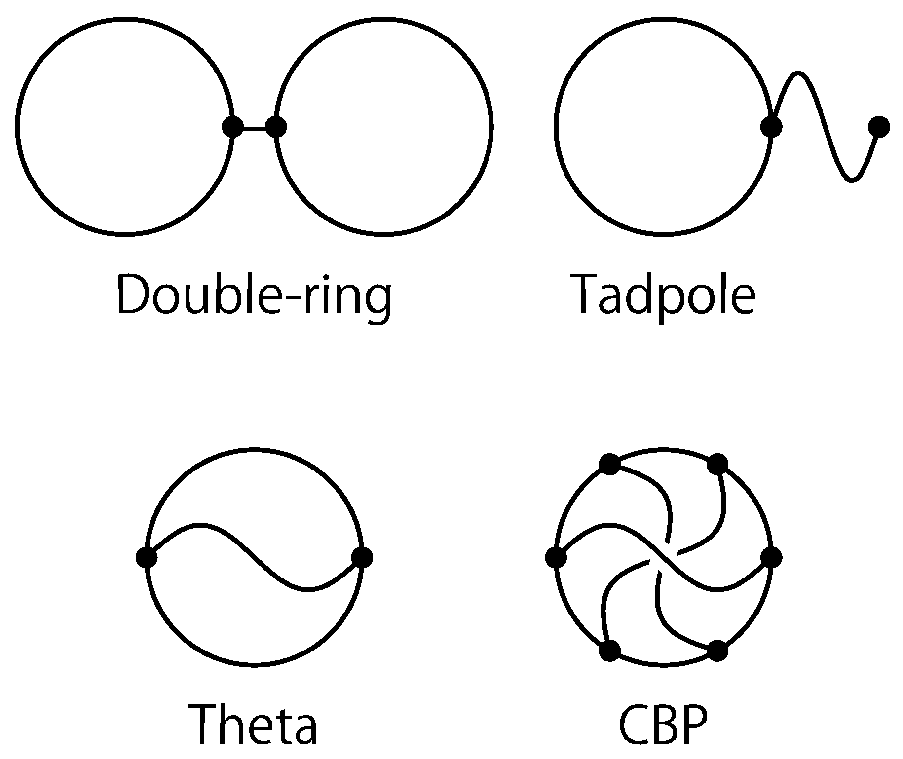
Figure 2.
Knot diagrams of the trivial knot , the trefoil knot , the figure-eight knot and the two prime knots and whose minimal crossing number is given by five.
Figure 2.
Knot diagrams of the trivial knot , the trefoil knot , the figure-eight knot and the two prime knots and whose minimal crossing number is given by five.
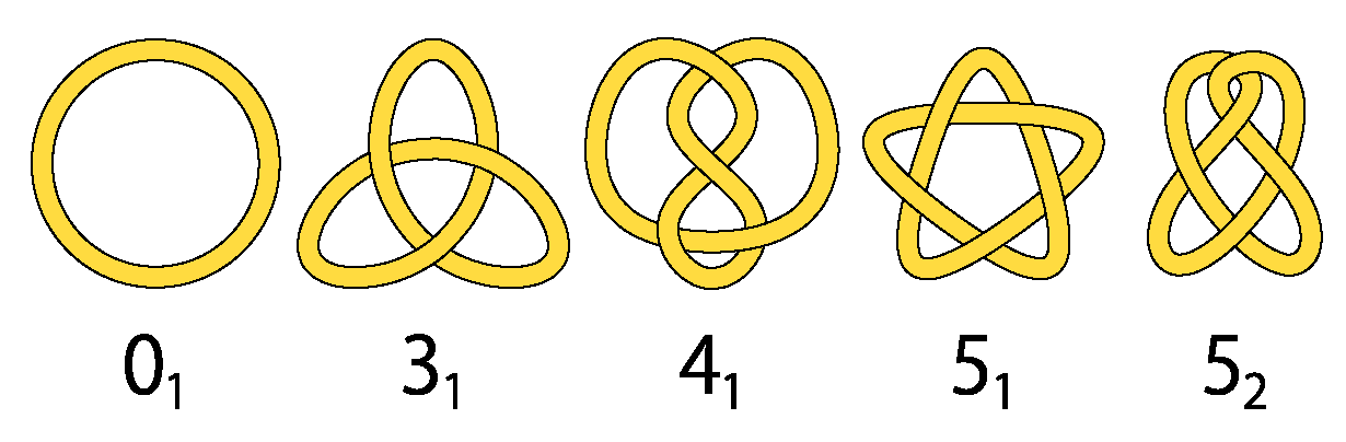
Figure 3.
Mean-square radius of gyration versus the number of segments N for ideal topological polymers with graph F evaluated by the quaternion method for six graphs F, such as linear, tadpole (lasso), ring, double-ring, -shaped and complete bipartite graph polymers, depicted by filled circles, filled diamonds, filled upper triangles, filled lower triangles, filled stars and filled squares, respectively. Each data point corresponds to the average over samples. The error bars are too small to be seen. Reprinted with permission from [31].

Figure 4.
Mean-square radius of gyration versus the number of segments N for real topological polymers with graphs F evaluated by the molecular dynamics of the Kremer–Grest model. Each data point corresponds to the average over samples. Reprinted with permission from [31].
Figure 4.
Mean-square radius of gyration versus the number of segments N for real topological polymers with graphs F evaluated by the molecular dynamics of the Kremer–Grest model. Each data point corresponds to the average over samples. Reprinted with permission from [31].
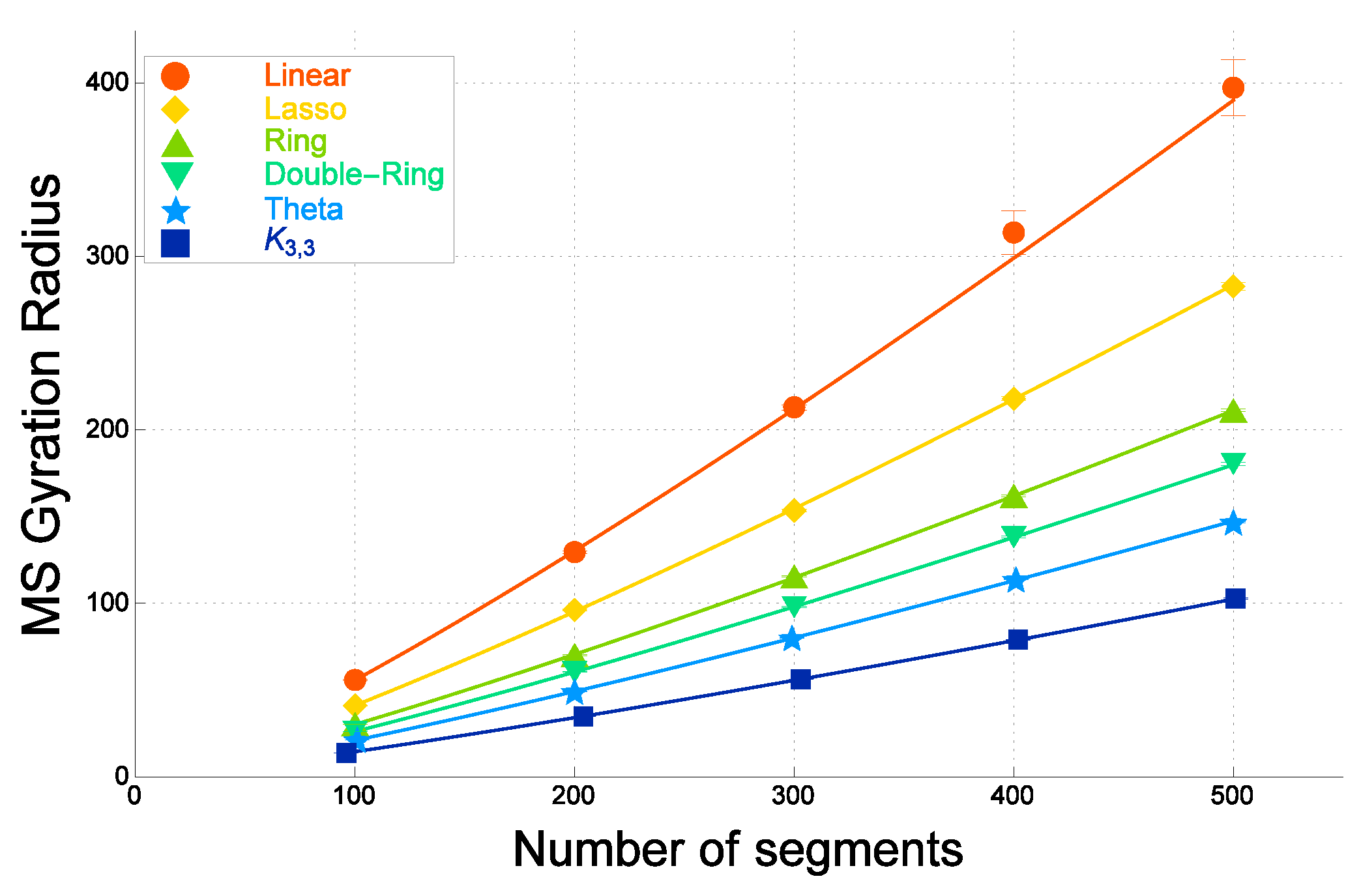
Figure 5.
Hydrodynamic radius squared versus the number of segments N for ideal topological polymers of graphs F evaluated by the quaternion method. The error bars are too small to be seen. Reprinted with permission from [31].
Figure 5.
Hydrodynamic radius squared versus the number of segments N for ideal topological polymers of graphs F evaluated by the quaternion method. The error bars are too small to be seen. Reprinted with permission from [31].

Figure 6.
Hydrodynamic radius squared versus the number of segments N for real topological polymers of graphs F (the Kremer–Grest model). The error bars are too small to be seen. Reprinted with permission from [31].
Figure 6.
Hydrodynamic radius squared versus the number of segments N for real topological polymers of graphs F (the Kremer–Grest model). The error bars are too small to be seen. Reprinted with permission from [31].
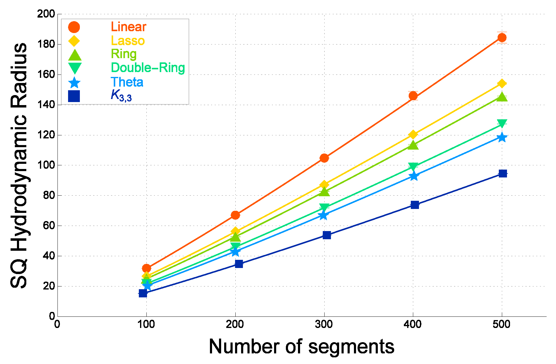
Figure 7.
Ratio of the gyration to hydrodynamic radii, , versus the number of segments N for ideal topological polymers with graphs F evaluated by the quaternion method. Reprinted with permission from [31].
Figure 7.
Ratio of the gyration to hydrodynamic radii, , versus the number of segments N for ideal topological polymers with graphs F evaluated by the quaternion method. Reprinted with permission from [31].
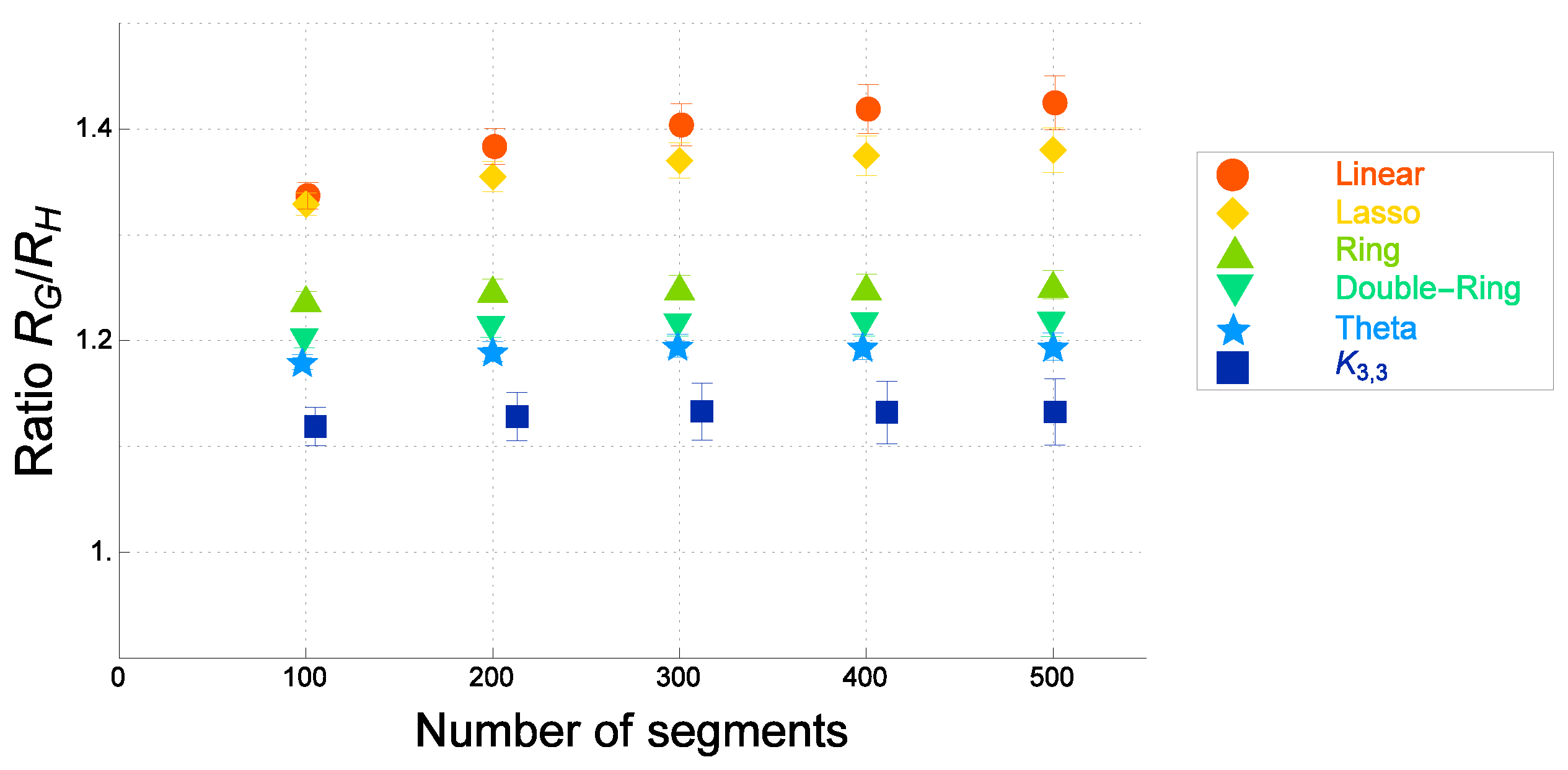
Figure 8.
Ratio of the gyration to hydrodynamic radii versus the number of segments N for real topological polymers (the Kremer–Grest model). Reprinted with permission from [31].
Figure 8.
Ratio of the gyration to hydrodynamic radii versus the number of segments N for real topological polymers (the Kremer–Grest model). Reprinted with permission from [31].
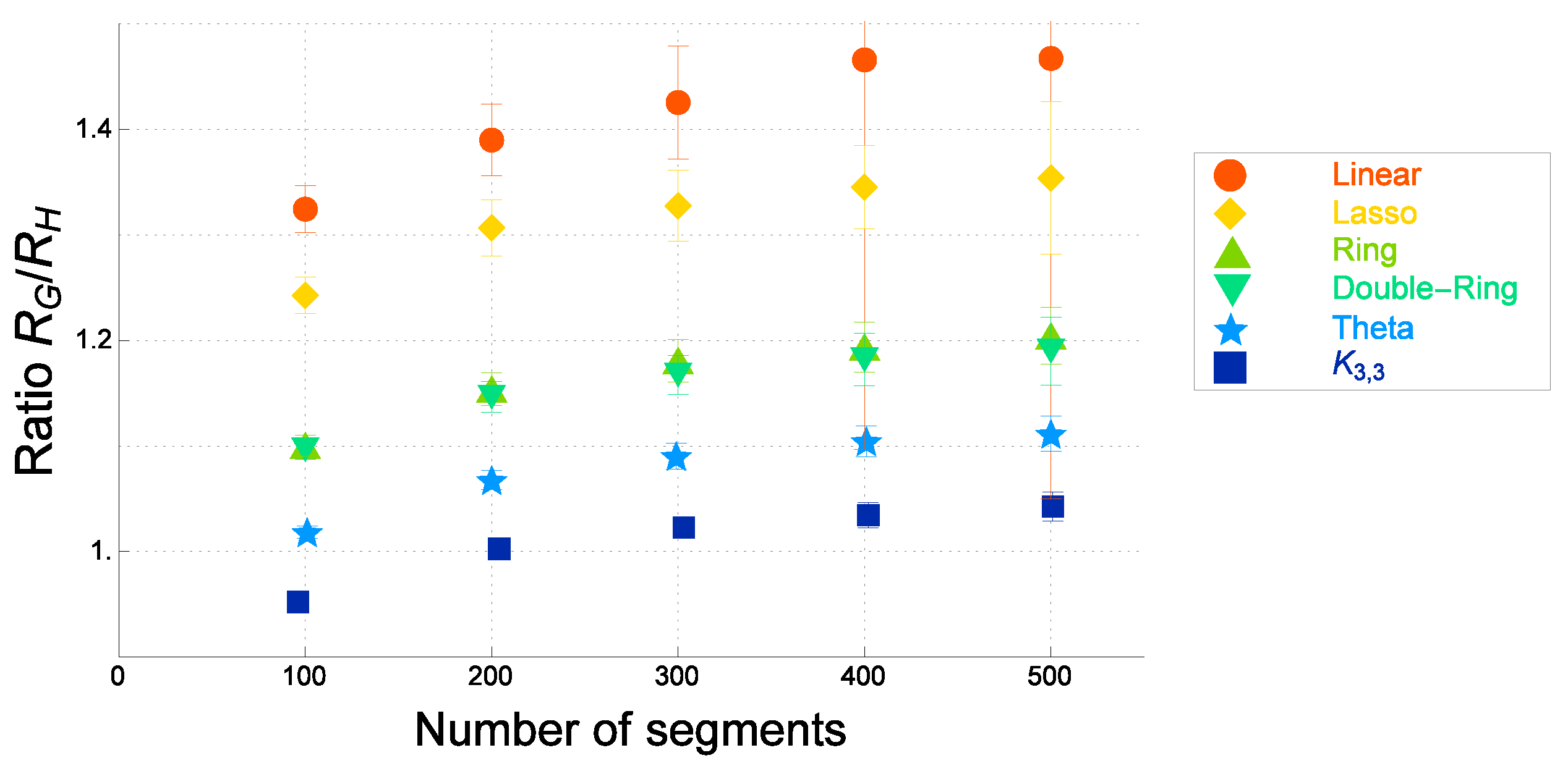
Figure 9.
Probability distribution function of the normalized distance x between any given pair of segments in an ideal topological polymer of with graph F, where the distance between two segments is normalized by the square root of the mean-square distance of the topological polymer with graph F. Here, graph F is given by a linear chain (red circles), a ring chain (green upper triangles), a theta curve (light blue stars) and a complete bipartite graph (dark blue squares). Reprinted with permission from [31].

Figure 10.
Double logarithmic plot of the probability distribution function of the normalized distance x between two segments in a real topological polymer (the Kremer–Grest model) of with graph F. The fitted lines are given by , , and for a linear (red circles), a ring (green upper triangles), a theta curve (light blue stars), and a complete bipartite graph polymer (dark blue squares), respectively. Reprinted with permission from [31].
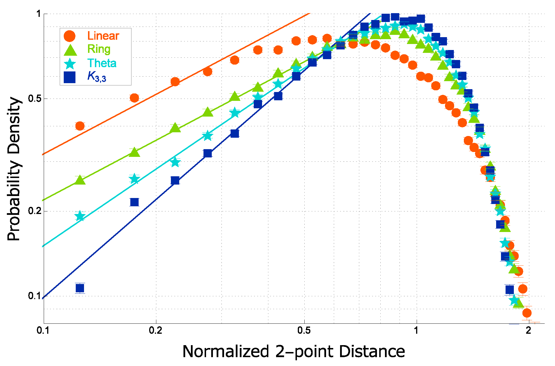
Figure 11.
Random polygon (or self-avoiding polygon) of N nodes corresponds to a conformation of a ring polymer chain in solution consisting of N statistical segments.
Figure 11.
Random polygon (or self-avoiding polygon) of N nodes corresponds to a conformation of a ring polymer chain in solution consisting of N statistical segments.
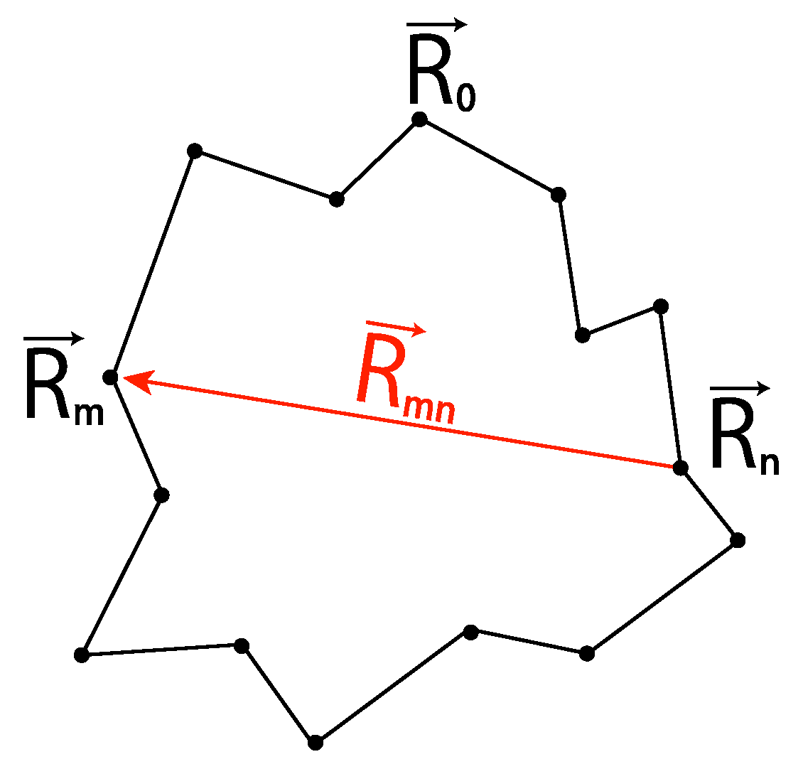
Figure 12.
Knotting probabilities of the trivial (), the trefoil () and the figure-eight () knots versus the number of segments N for cylindrical SAP with cylindrical radius . The knotting probabilities of knots and for the Gaussian random polygons with N up to 1600 are depicted in [66] with less good statistics.

Figure 13.
Knot diagram of a composite knot consisting of two trefoil knots ().

Figure 14.
Knotting probabilities of the trefoil knot () and its composite knots , , and with versus the number of segments N with good fitted curves for cylindrical self-avoiding polygons (SAP) with cylindrical radius . The knotting probabilities of composite knots such as , and are plotted for the Gaussian random polygons with N up to 1600 in less good statistics in [66].
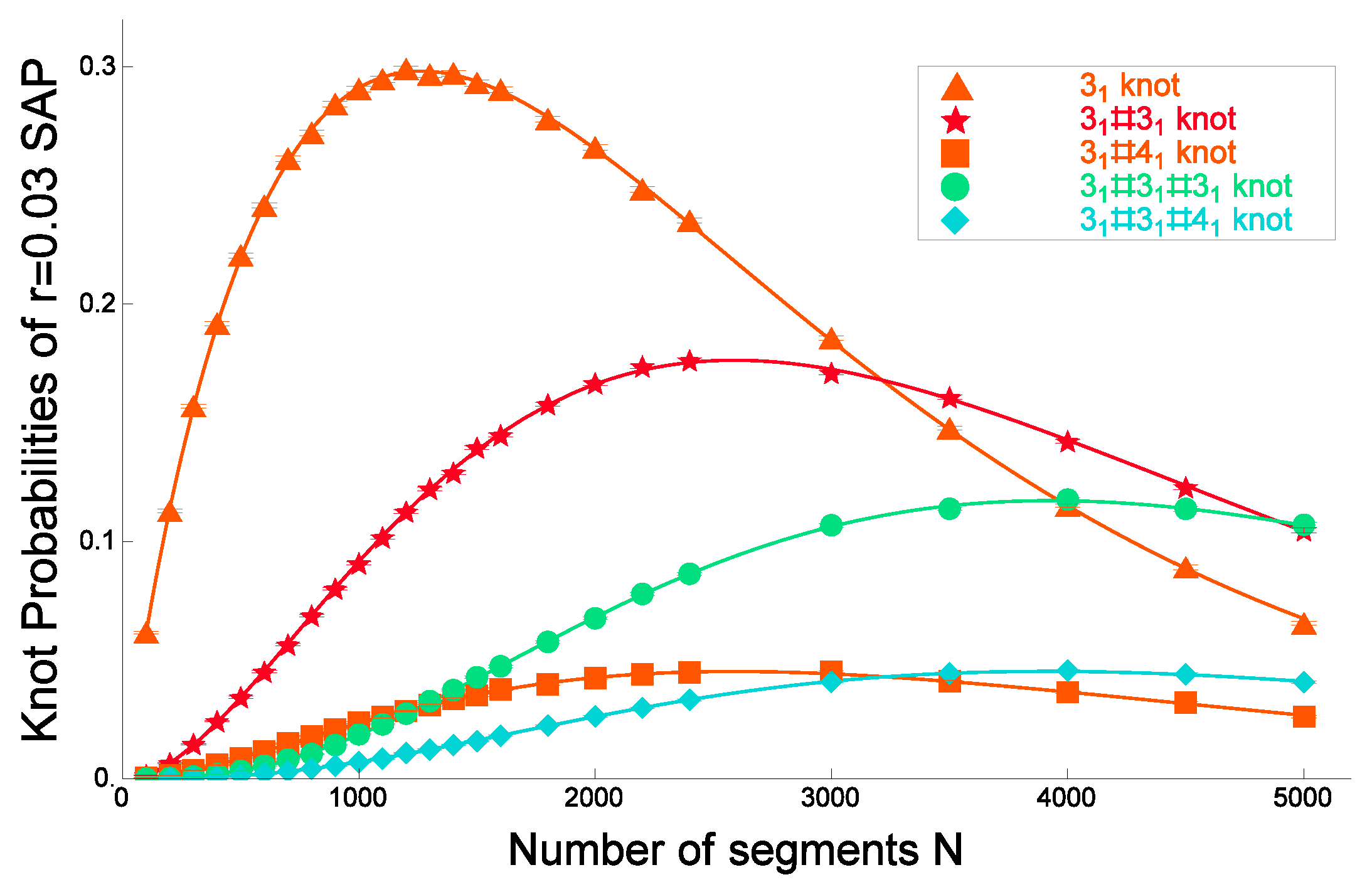
Figure 15.
Topological swelling of equilateral random polygons with fixed knot: Double logarithmic plots of the ratio of the mean-square radius of gyration of equilateral random polygon with a fixed knot K to that of no topological constraint, versus the number of segments N up to for the trivial knot (), the trefoil knot (), the figure-eight knot ) and the composite knot (). For the Gaussian random polygons with N less than 2000 the ratio is plotted against N in the double-logarithmic scale for knots , and in [88] with less good statistics.


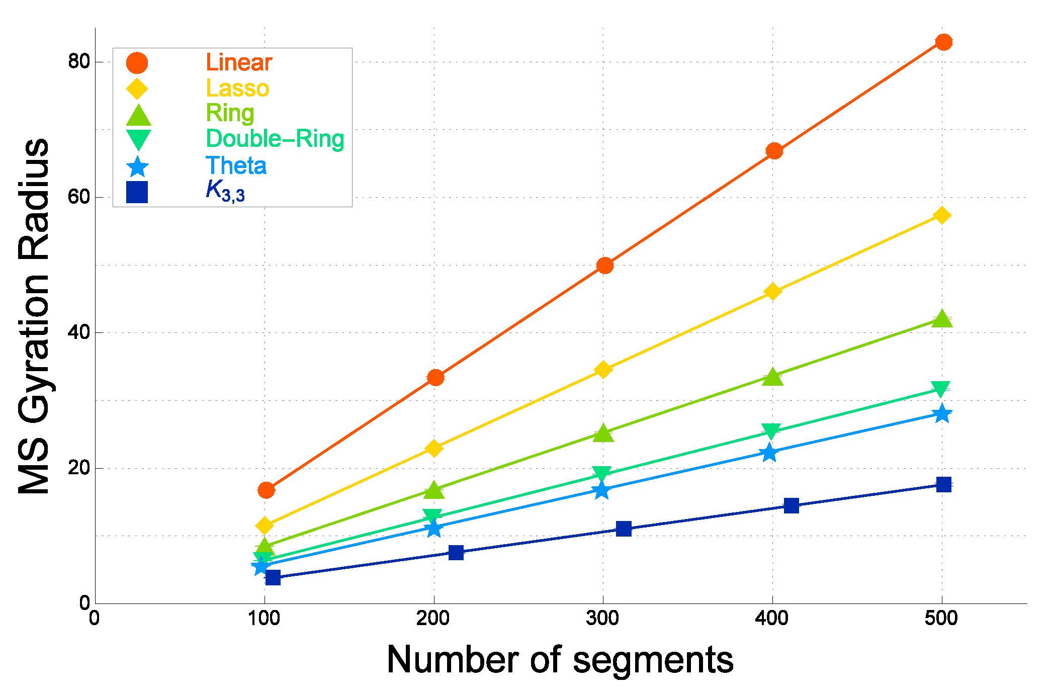
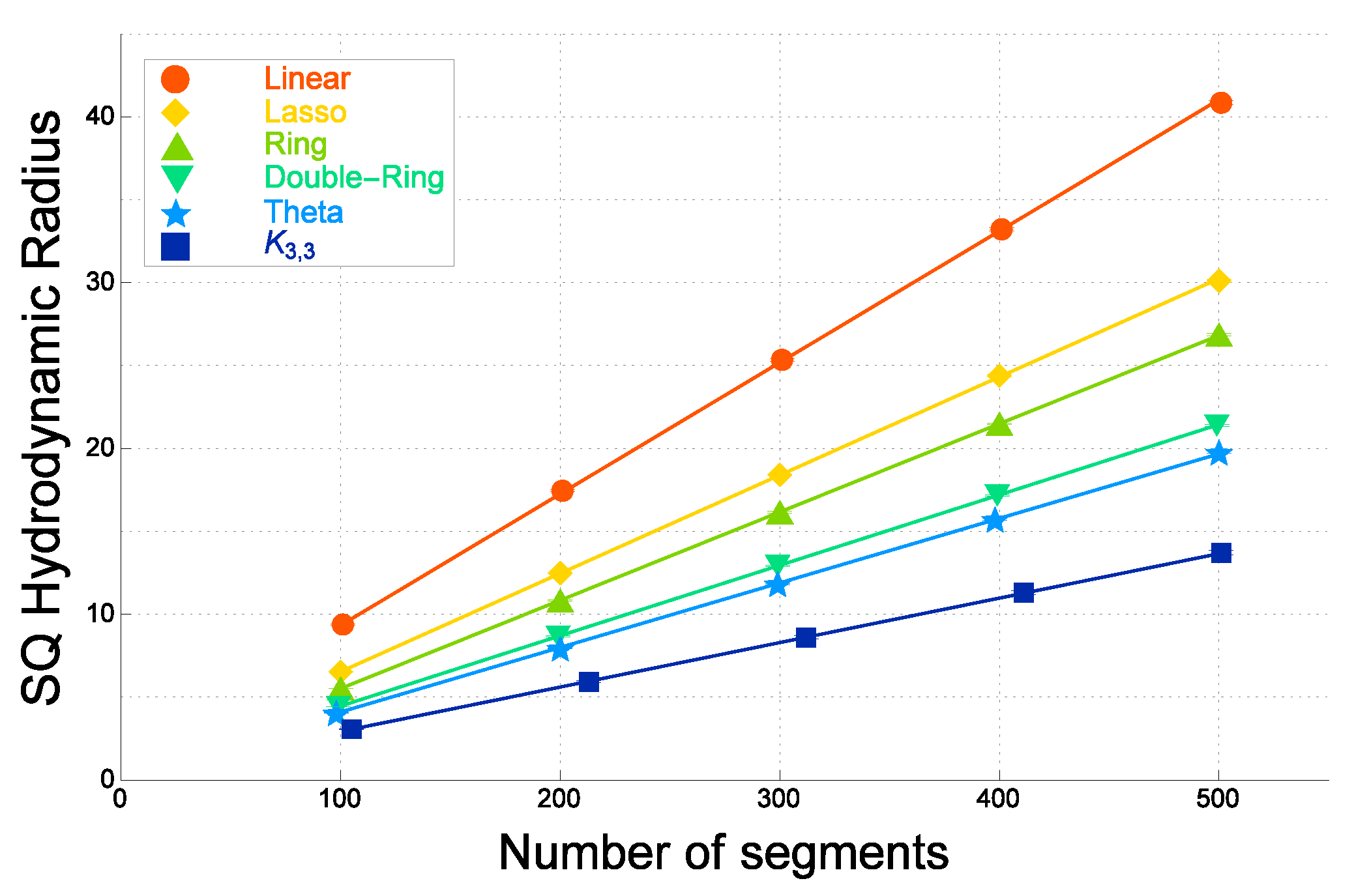
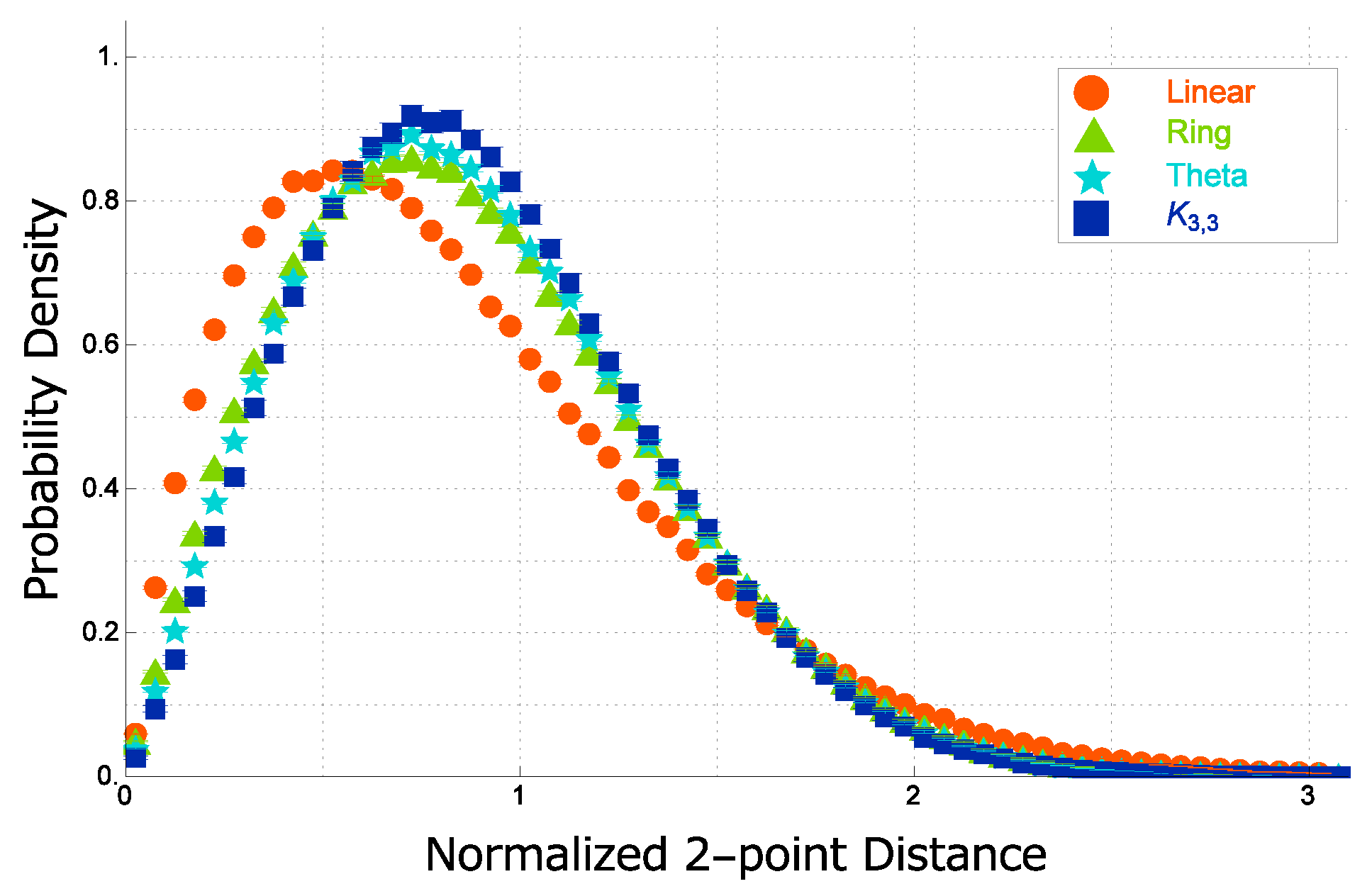
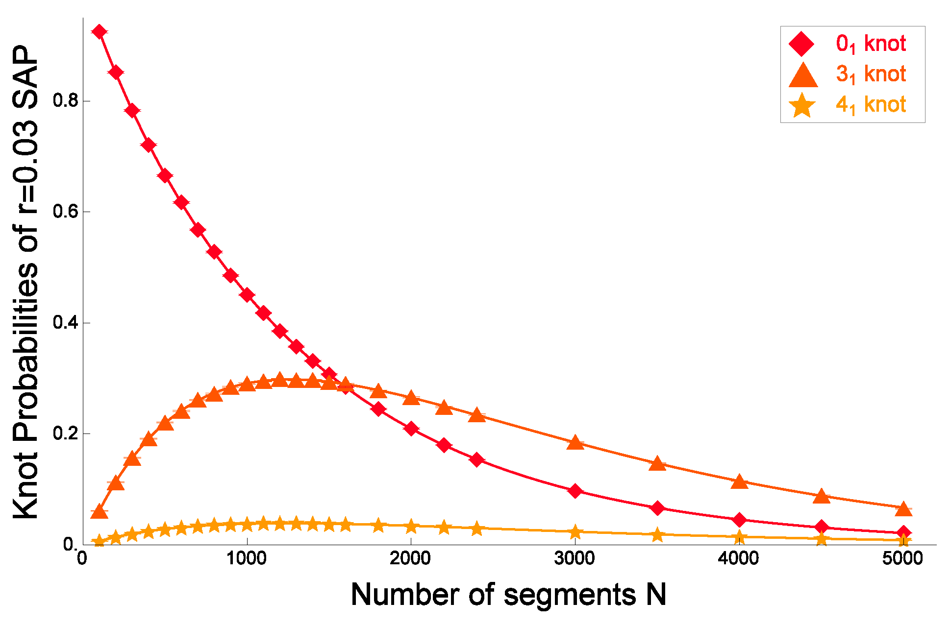
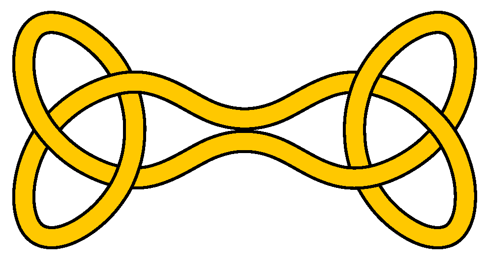
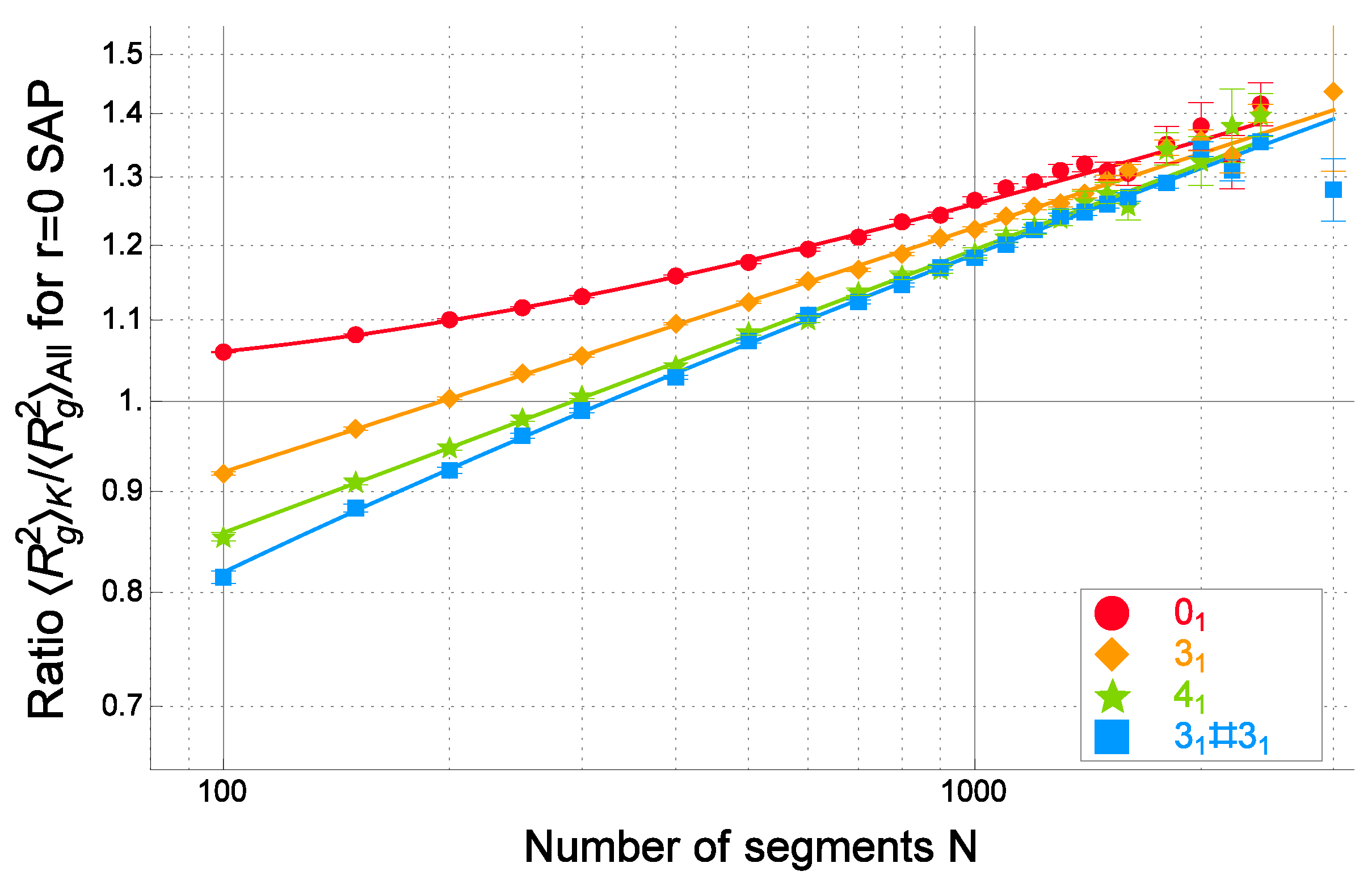
Table 1.
Ratio of coefficients, , in Equations (3) and (4) for ideal and real topological polymers with graphs F, respectively.
| Graph F | Ratio of (Ideal) | Ratio of (Real) |
|---|---|---|
| linear | ||
| tadpole (lasso) | ||
| ring | ||
| double-ring | ||
| -shaped | ||
| complete |
Table 2.
Ratio of the gyration radius to the hydrodynamic radius versus the number of segments N for ideal and real topological polymers with graph F.
Table 2.
Ratio of the gyration radius to the hydrodynamic radius versus the number of segments N for ideal and real topological polymers with graph F.
| Graph F | N | (Ideal) | (Real) |
|---|---|---|---|
| linear | 500 | ||
| tadpole (lasso) | 500 | ||
| ring | 500 | ||
| double-ring | 500 | ||
| -shaped | 500 | ||
| complete | 501 |
Table 3.
Values of the two knot invariants for some knots: the determinant of a knot (the Alexander polynomial evaluated at , ) and the Vassiliev invariant of the second degree, , for a knot type K.
Table 3.
Values of the two knot invariants for some knots: the determinant of a knot (the Alexander polynomial evaluated at , ) and the Vassiliev invariant of the second degree, , for a knot type K.
| Knot Type | |||||||
|---|---|---|---|---|---|---|---|
| Determinant of knot | 1 | 3 | 5 | 5 | 7 | 9 | 15 |
| 2nd order Vassiliev invariant | 0 | 1 | 3 | 2 | 2 | 0 |
© 2017 by the authors. Licensee MDPI, Basel, Switzerland. This article is an open access article distributed under the terms and conditions of the Creative Commons Attribution (CC BY) license (http://creativecommons.org/licenses/by/4.0/).
Share and Cite
MDPI and ACS Style
Deguchi, T.; Uehara, E. Statistical and Dynamical Properties of Topological Polymers with Graphs and Ring Polymers with Knots. Polymers 2017, 9, 252. https://doi.org/10.3390/polym9070252
AMA Style
Deguchi T, Uehara E. Statistical and Dynamical Properties of Topological Polymers with Graphs and Ring Polymers with Knots. Polymers. 2017; 9(7):252. https://doi.org/10.3390/polym9070252
Chicago/Turabian StyleDeguchi, Tetsuo, and Erica Uehara. 2017. "Statistical and Dynamical Properties of Topological Polymers with Graphs and Ring Polymers with Knots" Polymers 9, no. 7: 252. https://doi.org/10.3390/polym9070252
Note that from the first issue of 2016, this journal uses article numbers instead of page numbers. See further details here.