Recent Advances in Evapotranspiration Estimation Using Artificial Intelligence Approaches with a Focus on Hybridization Techniques—A Review


Abstract
:1. Introduction
2. Data Types
3. Artificial Intelligence Models
3.1. Artificial Neural Network (ANN)
- The evolution of the ANN from the MLP to the ELM was due to the constant need of improving training methods and algorithms in order to obtain effective predictions with greater accuracy, better generalization and lesser dependency on input parameters.
- Within each and every variation of the ANN model, one could safely and easily deduce that the trend and focus of study would not deviate much from the following four aspects:
- Minimization of required input parameters,
- Generalization of the ANN for wider spatial application,
- Introduction of new input parameters,
- Enhancement of ANN prediction ability.
- 3.
- Longer forecasting horizon could provide a good pre-requisite for effective water allocation strategy. The use of the ANN alone could sometimes be insufficient to provide a solution for the above aspects.
- 4.
- The black-box operation of ANN could not offer an explanation to the complex ET process.
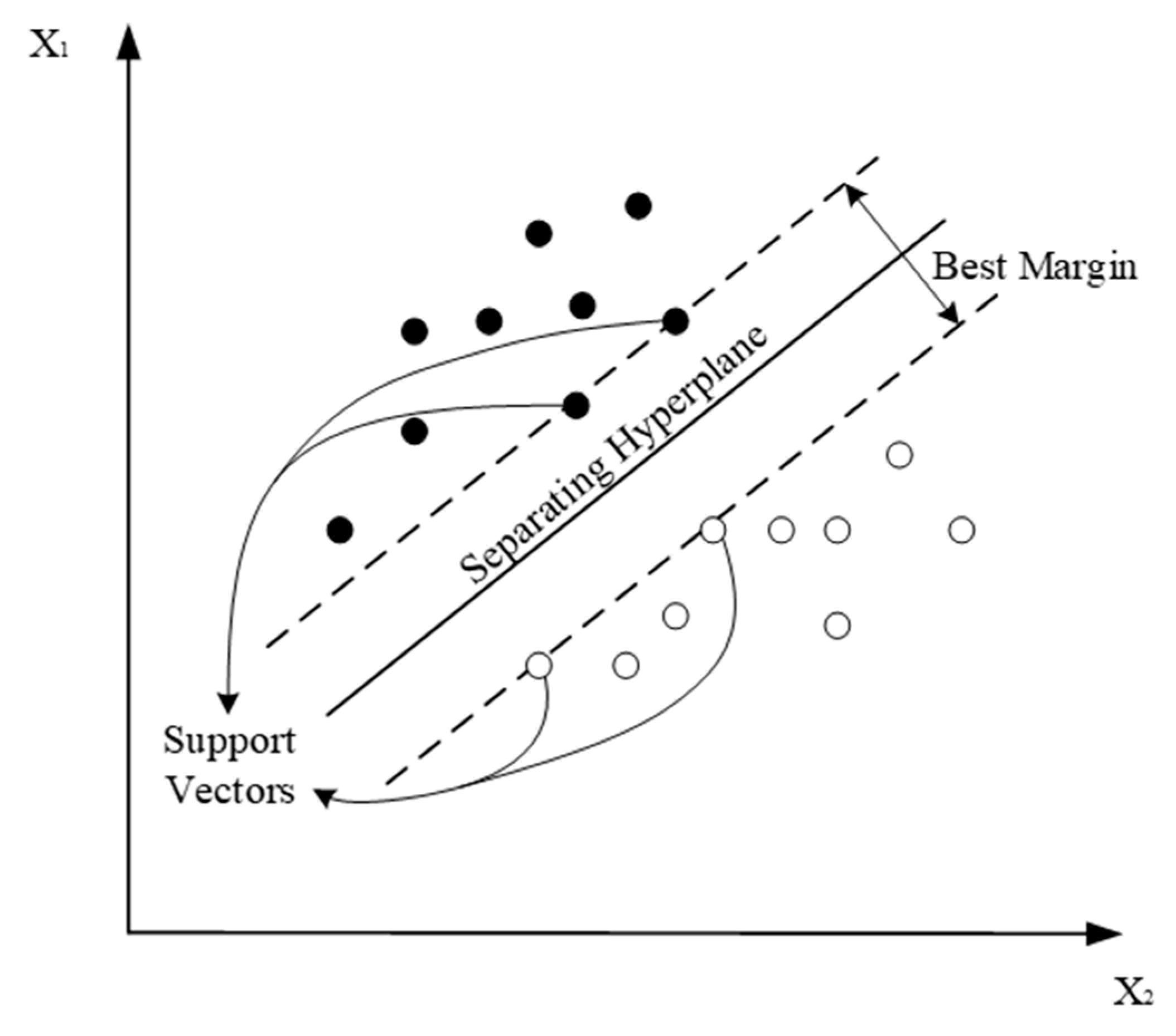
3.2. Support Vector Machine (SVM)
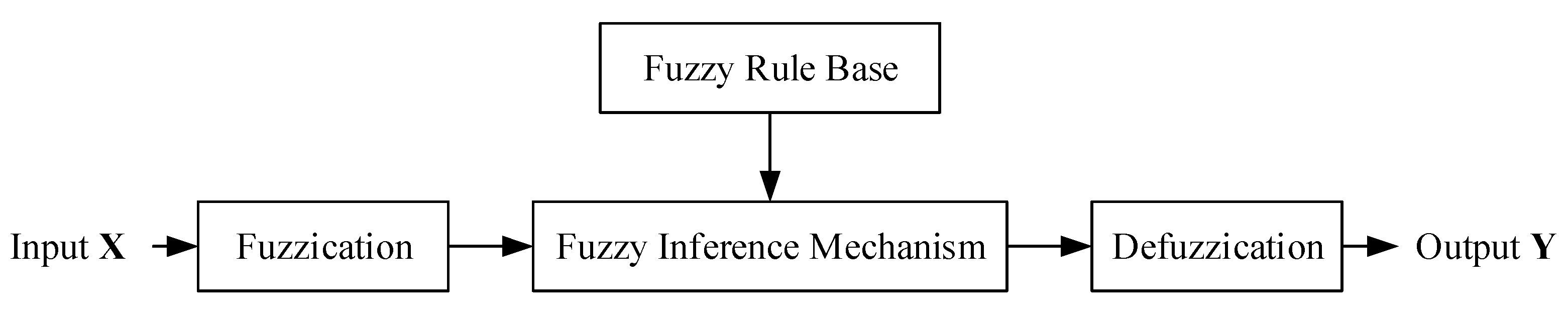
3.3. Fuzzy Models
3.4. Tree Based Models
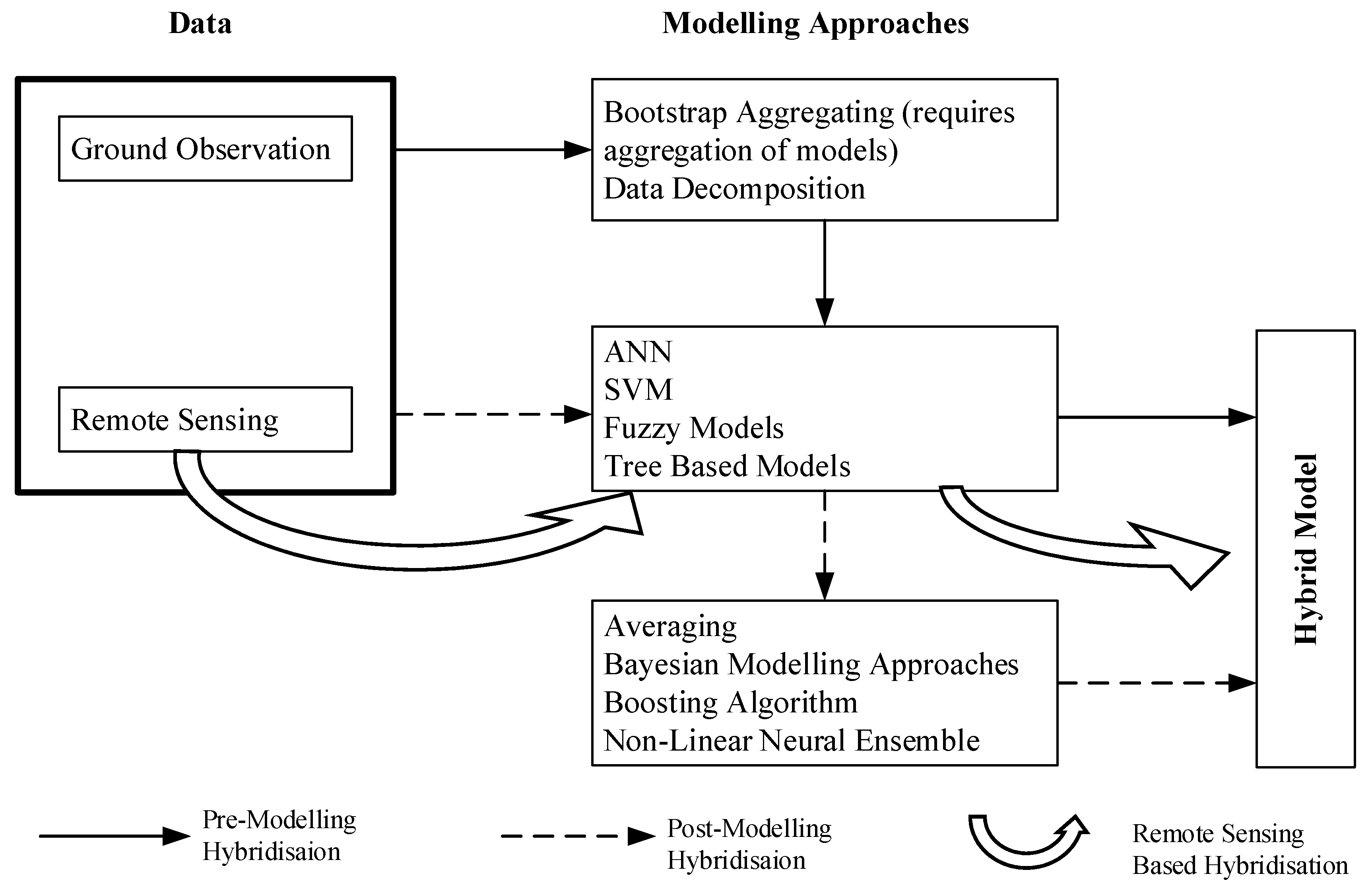
4. Hybrid Models
4.1. Data Fusion and Ensemble Modelling
4.1.1. Averaging
4.1.2. Bootstrap Aggregating
4.1.3. Bayesian Modeling Approaches
4.1.4. Boosting Algorithm
4.1.5. Nonlinear Neural Ensemble
4.1.6. Ensemble Models for Remote Sensing
4.2. Data Decomposition
5. Future Prospects
6. Conclusions
Author Contributions
Funding
Conflicts of Interest
Nomenclature
| ANFIS | adaptive neuro-fuzzy inference system |
| ANN | artificial neural network |
| BPNN | back-propagation neural network |
| ELM | extreme learning machine |
| ESTARFM | enhanced spatial and temporal adaptive reflectance fusion model ET evapotranspiration |
| ET0 | reference evapotranspiration |
| FIS | fuzzy inference system |
| GLASS | global land surface satellite |
| GRNN | generalised regression neural network |
| HS | Hargreaves–Samani |
| Kc | crop coefficient |
| LDAS | land data assimilation system |
| MLP | multilayer layer perceptron |
| MODIS | Moderate Resolution Imaging Spectroradiometer |
| PET | potential evapotranspiration |
| PM | Penman–Monteith |
| PT | Priestley–Taylor |
| RBF | radial basis function |
| RVM | relevance vector machine |
| SEBS | surface energy balance system |
| STARFM | spatial and temporal adaptive reflectance fusion model |
| SVM | support vector machines |
| SVR | support vector regression |
| WNN | wavelet neural network |
References
- United Nations. World Population Prospects: The 2019 Highlights; ST/ESA/SER.A/423; Department of Economic and Social Affairs/Population Division: New York, NY, USA, 2019. [Google Scholar]
- Cascone, S.; Coma, J.; Gagliano, A.; Pérez, G. The evapotranspiration process in green roofs: A review. Build. Environ. 2019, 147, 337–355. [Google Scholar] [CrossRef]
- Stanhill, G. Evapotranspiration. In Encyclopedia of Soils in the Environment; Hillel, D., Ed.; Elsevier: Amsterdam, The Netherlands, 2005; pp. 502–506. [Google Scholar]
- Jovic, S.; Nedeljkovic, B.; Golubovic, Z.; Kostic, N. Evolutionary algorithm for reference evapotranspiration analysis. Comput. Electron. Agric. 2018, 150, 1–4. [Google Scholar] [CrossRef]
- Granata, F. Evapotranspiration evaluation models based on machine learning algorithms—A comparative study. Agric. Water Manag. 2019, 217, 303–315. [Google Scholar] [CrossRef]
- Holmes, J.W. Measuring evapotranspiration by hydrological methods. Agric. Water Manag. 1984, 8, 29–40. [Google Scholar] [CrossRef]
- Pokorny, J. Evapotranspiration. In Encyclopedia of Ecology, 2nd ed.; Fath, B., Ed.; Elsevier: Amsterdam, The Netherlands, 2019; Volume 2, pp. 292–303. [Google Scholar]
- Wang, K.; Dickinson, R.E. A review of global terrestrial evapotranspiration: Observation, modeling, climatology, and climatic variability. Rev. Geophys. 2012, 50, RG2005. [Google Scholar] [CrossRef]
- Anapalli, S.S.; Ahuja, L.R.; Gowda, P.H.; Ma, L.; Marek, G.; Evett, S.R.; Howell, T.A. Simulation of crop evapotranspiration and crop coefficients with data in weighing lysimeters. Agric. Water Manag. 2016, 177, 274–283. [Google Scholar] [CrossRef] [Green Version]
- Liu, X.; Xu, C.; Zhong, X.; Li, Y.; Yuan, X.; Cao, J. Comparison of 16 models for reference crop evapotranspiration against weighing lysimeter measurement. Agric. Water Manag. 2017, 184, 145–155. [Google Scholar] [CrossRef]
- Pereira, L.S.; Allen, R.G.; Smith, M.; Raes, D. Crop evapotranspiration estimation with FAO56: Past and future. Agric. Water Manag. 2015, 147, 4–20. [Google Scholar] [CrossRef]
- Monteith, J.L. Evaporation and the environment in the state and movement of water in living organisms. In Proceedings of the Society for Experimental Biology, Symposium No. 19, Cambridge, UK, 1 January 1965; Cambridge University Press: Cambridge, UK, 1965; pp. 205–234. [Google Scholar]
- Allan, R.G.; Pereira, L.; Raes, D.; Smith, M. Crop Evapotranspiration—Guidelines for Computing Crop Water Requirements—FAO Irrigation and Drainage Paper 56; Food and Agriculture Organization of the United Nations: Rome, Italy, 1998; Volume 56. [Google Scholar]
- Saggi, M.K.; Jain, S. Reference evapotranspiration estimation and modeling of the Punjab Northern India using deep learning. Comput. Electron. Agric. 2019, 156, 387–398. [Google Scholar] [CrossRef]
- Shiri, J.; Marti, P.; Karimi, S.; Landeras, G. Data splitting strategies for improving data driven models for reference evapotranspiration estimation among similar stations. Comput. Electron. Agric. 2019, 162, 70–81. [Google Scholar] [CrossRef]
- Güçlü, Y.S.; Subyani, A.M.; Şen, Z. Regional fuzzy chain model for evapotranspiration estimation. J. Hydrol. 2017, 544, 233–241. [Google Scholar] [CrossRef]
- Hargreaves, G.H.; Samani, Z.A. Reference Crop Evapotranspiration from Temperature. Appl. Eng. Agric. 1985, 1, 96–99. [Google Scholar] [CrossRef]
- Luo, Y.; Chang, X.; Peng, S.; Khan, S.; Wang, W.; Zheng, Q.; Cai, X. Short-term forecasting of daily reference evapotranspiration using the Hargreaves–Samani model and temperature forecasts. Agric. Water Manag. 2014, 136, 42–51. [Google Scholar] [CrossRef]
- Berti, A.; Tardivo, G.; Chiaudani, A.; Rech, F.; Borin, M. Assessing reference evapotranspiration by the Hargreaves method in north-eastern Italy. Agric. Water Manag. 2014, 140, 20–25. [Google Scholar] [CrossRef]
- Priestley, C.H.B.; Taylor, R.J. On the Assessment of Surface Heat Flux and Evaporation Using Large-Scale Parameters. Mon. Weather Rev. 1972, 100, 81–92. [Google Scholar] [CrossRef]
- Liu, J.G.; Zhao, T.S.; Chen, R.; Wong, C.W. The effect of methanol concentration on the performance of a passive DMFC. Electrochem. Commun. 2005, 7, 288–294. [Google Scholar] [CrossRef]
- Turc, L. Water requirements assessment of irrigation, potential evapotranspiration: Simplified and updated climatic formula. Ann. Agron. 1961, 12, 13–49. [Google Scholar]
- Thornthwaite, C.W. An Approach toward a Rational Classification of Climate. Geogr. Rev. 1948, 38, 55. [Google Scholar] [CrossRef]
- Liu, S.; Xu, Z.; Song, L.; Zhao, Q.; Ge, Y.; Xu, T.; Ma, Y.; Zhu, Z.; Jia, Z.; Zhang, F. Upscaling evapotranspiration measurements from multi-site to the satellite pixel scale over heterogeneous land surfaces. Agric. For. Meteorol. 2016, 230–231, 97–113. [Google Scholar] [CrossRef]
- Valipour, M.; Gholami Sefidkouhi, M.A.; Raeini-Sarjaz, M.; Guzman, S.M. A Hybrid Data-Driven Machine Learning Technique for Evapotranspiration Modeling in Various Climates. Atmosphere 2019, 10, 311. [Google Scholar] [CrossRef] [Green Version]
- Wang, S.; Fu, Z.-Y.; Chen, H.-S.; Nie, Y.-P.; Wang, K.-L. Modeling daily reference ET in the karst area of northwest Guangxi (China) using gene expression programming (GEP) and artificial neural network (ANN). Theor. Appl. Climatol. 2015, 126, 493–504. [Google Scholar] [CrossRef]
- Falamarzi, Y.; Palizdan, N.; Huang, Y.F.; Lee, T.S. Estimating evapotranspiration from temperature and wind speed data using artificial and wavelet neural networks (WNNs). Agric. Water Manag. 2014, 140, 26–36. [Google Scholar] [CrossRef]
- Tabari, H.; Hosseinzadeh Talaee, P. Multilayer perceptron for reference evapotranspiration estimation in a semiarid region. Neural Comput. Appl. 2012, 23, 341–348. [Google Scholar] [CrossRef]
- Kisi, O.; Alizamir, M. Modelling reference evapotranspiration using a new wavelet conjunction heuristic method: Wavelet extreme learning machine vs. wavelet neural networks. Agric. For. Meteorol. 2018, 263, 41–48. [Google Scholar] [CrossRef]
- Abdullah, S.S.; Malek, M.A.; Abdullah, N.S.; Kisi, O.; Yap, K.S. Extreme Learning Machines: A new approach for prediction of reference evapotranspiration. J. Hydrol. 2015, 527, 184–195. [Google Scholar] [CrossRef]
- Huo, Z.; Feng, S.; Kang, S.; Dai, X. Artificial neural network models for reference evapotranspiration in an arid area of northwest China. J. Arid Environ. 2012, 82, 81–90. [Google Scholar] [CrossRef]
- Wen, X.; Si, J.; He, Z.; Wu, J.; Shao, H.; Yu, H. Support-Vector-Machine-Based Models for Modeling Daily Reference Evapotranspiration With Limited Climatic Data in Extreme Arid Regions. Water Resour. Manag. 2015, 29, 3195–3209. [Google Scholar] [CrossRef]
- Nourani, V.; Elkiran, G.; Abdullahi, J. Multi-station artificial intelligence based ensemble modeling of reference evapotranspiration using pan evaporation measurements. J. Hydrol. 2019, 577, 123958. [Google Scholar] [CrossRef]
- Feng, Y.; Gong, D.; Mei, X.; Cui, N. Estimation of maize evapotranspiration using extreme learning machine and generalized regression neural network on the China Loess Plateau. Hydrol. Res. 2017, 48, 1156–1168. [Google Scholar] [CrossRef]
- Huang, G.; Wu, L.; Ma, X.; Zhang, W.; Fan, J.; Yu, X.; Zeng, W.; Zhou, H. Evaluation of CatBoost method for prediction of reference evapotranspiration in humid regions. J. Hydrol. 2019, 574, 1029–1041. [Google Scholar] [CrossRef]
- Ladlani, I.; Houichi, L.; Djemili, L.; Heddam, S.; Belouz, K. Modeling daily reference evapotranspiration (ET0) in the north of Algeria using generalized regression neural networks (GRNN) and radial basis function neural networks (RBFNN): A comparative study. Meteorol. Atmos. Phys. 2012, 118, 163–178. [Google Scholar] [CrossRef]
- Yamaç, S.S.; Todorovic, M. Estimation of daily potato crop evapotranspiration using three different machine learning algorithms and four scenarios of available meteorological data. Agric. Water Manag. 2020, 228, 105875. [Google Scholar] [CrossRef]
- Maeda, E.E.; Wiberg, D.A.; Pellikka, P.K.E. Estimating reference evapotranspiration using remote sensing and empirical models in a region with limited ground data availability in Kenya. Appl. Geogr. 2011, 31, 251–258. [Google Scholar] [CrossRef]
- National Aeronautics and Space Administration FLUXNET. Available online: https://daac.ornl.gov/cgi-bin/dataset_lister.pl?p=9 (accessed on 23 October 2019).
- Yang, F.; White, M.A.; Michaelis, A.R.; Ichii, K.; Hashimoto, H.; Votava, P.; Zhu, A.X.; Nemani, R.R. Prediction of Continental-Scale Evapotranspiration by Combining MODIS and AmeriFlux Data Through Support Vector Machine. IEEE Trans. Geosci. Remote Sens. 2006, 44, 3452–3461. [Google Scholar] [CrossRef]
- Nagler, P.; Scott, R.; Westenburg, C.; Cleverly, J.; Glenn, E.; Huete, A. Evapotranspiration on western U.S. rivers estimated using the Enhanced Vegetation Index from MODIS and data from eddy covariance and Bowen ratio flux towers. Remote Sens. Environ. 2005, 97, 337–351. [Google Scholar] [CrossRef]
- Rodell, M.; Houser, P.R.; Jambor, U.; Gottschalck, J.; Mitchell, K.; Meng, C.J.; Arsenault, K.; Cosgrove, B.; Radakovich, J.; Bosilovich, M.; et al. The Global Land Data Assimilation System. Bull. Am. Meteorol. Soc. 2004, 85, 381–394. [Google Scholar] [CrossRef] [Green Version]
- Abiodun, O.I.; Jantan, A.; Omolara, A.E.; Dada, K.V.; Mohamed, N.A.; Arshad, H. State-of-the-art in artificial neural network applications: A survey. Heliyon 2018, 4, e00938. [Google Scholar] [CrossRef] [Green Version]
- Rosenblatt, F. The perceptron: A probabilistic model for information storage and organization in the brain. Psychol. Rev. 1958, 65, 386–408. [Google Scholar] [CrossRef] [Green Version]
- Hornik, K.; Stinchcombe, M.; White, H. Multilayer feedforward networks are universal approximators. Neural Netw. 1989, 2, 359–366. [Google Scholar] [CrossRef]
- Lek, S.; Guégan, J.F. Artificial neural networks as a tool in ecological modelling, an introduction. Ecol. Model. 1999, 120, 65–73. [Google Scholar] [CrossRef]
- Kumar, M.; Raghuwanshi, N.S.; Singh, R.; Wallender, W.W.; Pruitt, W.O. Estimating Evapotranspiration using Artificial Neural Network. J. Irrig. Drain. Eng. 2002, 128, 224–233. [Google Scholar] [CrossRef]
- Rahimikhoob, A. Estimation of evapotranspiration based on only air temperature data using artificial neural networks for a subtropical climate in Iran. Theor. Appl. Climatol. 2009, 101, 83–91. [Google Scholar] [CrossRef]
- Antonopoulos, V.Z.; Antonopoulos, A.V. Daily reference evapotranspiration estimates by artificial neural networks technique and empirical equations using limited input climate variables. Comput. Electron. Agric. 2017, 132, 86–96. [Google Scholar] [CrossRef]
- Reis, M.M.; da Silva, A.J.; Zullo Junior, J.; Tuffi Santos, L.D.; Azevedo, A.M.; Lopes, É.M.G. Empirical and learning machine approaches to estimating reference evapotranspiration based on temperature data. Comput. Electron. Agric. 2019, 165, 104937. [Google Scholar] [CrossRef]
- Citakoglu, H.; Cobaner, M.; Haktanir, T.; Kisi, O. Estimation of Monthly Mean Reference Evapotranspiration in Turkey. Water Resour. Manag. 2013, 28, 99–113. [Google Scholar] [CrossRef]
- Rahimikhoob, A. Comparison between M5 Model Tree and Neural Networks for Estimating Reference Evapotranspiration in an Arid Environment. Water Resour. Manag. 2014, 28, 657–669. [Google Scholar] [CrossRef]
- Shiri, J.; Nazemi, A.H.; Sadraddini, A.A.; Landeras, G.; Kisi, O.; Fakheri Fard, A.; Marti, P. Comparison of heuristic and empirical approaches for estimating reference evapotranspiration from limited inputs in Iran. Comput. Electron. Agric. 2014, 108, 230–241. [Google Scholar] [CrossRef]
- Pandey, P.K.; Nyori, T.; Pandey, V. Estimation of reference evapotranspiration using data driven techniques under limited data conditions. Model. Earth Syst. Environ. 2017, 3, 1449–1461. [Google Scholar] [CrossRef]
- Broomhead, D.S.; A Lowe, D. Multivariable functional interpolation and adaptive networks. Complex Syst. 1988, 2, 321–355. [Google Scholar]
- Specht, D.F. A general regression neural network. IEEE Trans. Neural Netw. 1991, 2, 568–576. [Google Scholar] [CrossRef] [Green Version]
- Huang, G.-B.; Zhu, Q.-Y.; Siew, C.-K. Extreme learning machine: Theory and applications. Neurocomputing 2006, 70, 489–501. [Google Scholar] [CrossRef]
- Trajkovic, S. Comparison of radial basis function networks and empirical equations for converting from pan evaporation to reference evapotranspiration. Hydrol. Process. 2009, 23, 874–880. [Google Scholar] [CrossRef]
- Feng, Y.; Cui, N.; Gong, D.; Zhang, Q.; Zhao, L. Evaluation of random forests and generalized regression neural networks for daily reference evapotranspiration modelling. Agric. Water Manag. 2017, 193, 163–173. [Google Scholar] [CrossRef]
- Feng, Y.; Peng, Y.; Cui, N.; Gong, D.; Zhang, K. Modeling reference evapotranspiration using extreme learning machine and generalized regression neural network only with temperature data. Comput. Electron. Agric. 2017, 136, 71–78. [Google Scholar] [CrossRef]
- Traore, S.; Wang, Y.-M.; Kerh, T. Artificial neural network for modeling reference evapotranspiration complex process in Sudano-Sahelian zone. Agric. Water Manag. 2010, 97, 707–714. [Google Scholar] [CrossRef]
- Yassin, M.A.; Alazba, A.A.; Mattar, M.A. Artificial neural networks versus gene expression programming for estimating reference evapotranspiration in arid climate. Agric. Water Manag. 2016, 163, 110–124. [Google Scholar] [CrossRef]
- Rahimikhoob, A. Comparison of M5 Model Tree and Artificial Neural Network’s Methodologies in Modelling Daily Reference Evapotranspiration from NOAA Satellite Images. Water Resour. Manag. 2016, 30, 3063–3075. [Google Scholar] [CrossRef]
- Gocic, M.; Petković, D.; Shamshirband, S.; Kamsin, A. Comparative analysis of reference evapotranspiration equations modelling by extreme learning machine. Comput. Electron. Agric. 2016, 127, 56–63. [Google Scholar] [CrossRef]
- Patil, A.P.; Deka, P.C. An extreme learning machine approach for modeling evapotranspiration using extrinsic inputs. Comput. Electron. Agric. 2016, 121, 385–392. [Google Scholar] [CrossRef]
- Hashemi, M.; Sepaskhah, A.R. Evaluation of artificial neural network and Penman–Monteith equation for the prediction of barley standard evapotranspiration in a semi-arid region. Theor. Appl. Climatol. 2019. [Google Scholar] [CrossRef]
- Abrishami, N.; Sepaskhah, A.R.; Shahrokhnia, M.H. Estimating wheat and maize daily evapotranspiration using artificial neural network. Theor. Appl. Climatol. 2018, 135, 945–958. [Google Scholar] [CrossRef]
- Vapnik, V. The Nature of Statistical Learning Theory, 2nd ed.; Springer-Verlag: New York, NY, USA, 1995. [Google Scholar]
- Cortes, C.; Vapnik, V. Support-vector networks. Mach. Learn. 1995, 20, 273–297. [Google Scholar] [CrossRef]
- Raghavendra, N.S.; Deka, P.C. Support vector machine applications in the field of hydrology: A review. Appl. Soft Comput. 2014, 19, 372–386. [Google Scholar] [CrossRef]
- Zendehboudi, A.; Baseer, M.A.; Saidur, R. Application of support vector machine models for forecasting solar and wind energy resources: A review. J. Clean. Prod. 2018, 199, 272–285. [Google Scholar] [CrossRef]
- Kisi, O.; Cimen, M. Evapotranspiration modelling using support vector machines. Hydrol. Sci. J. 2010, 54, 918–928. [Google Scholar] [CrossRef]
- Mehdizadeh, S.; Behmanesh, J.; Khalili, K. Using MARS, SVM, GEP and empirical equations for estimation of monthly mean reference evapotranspiration. Comput. Electron. Agric. 2017, 139, 103–114. [Google Scholar] [CrossRef]
- Mohammadrezapour, O.; Piri, J.; Kisi, O. Comparison of SVM, ANFIS and GEP in modeling monthly potential evapotranspiration in an arid region (Case study: Sistan and Baluchestan Province, Iran). Water Supply 2019, 19, 392–403. [Google Scholar] [CrossRef] [Green Version]
- Ferreira, L.B.; da Cunha, F.F.; de Oliveira, R.A.; Fernandes Filho, E.I. Estimation of reference evapotranspiration in Brazil with limited meteorological data using ANN and SVM—A new approach. J. Hydrol. 2019, 572, 556–570. [Google Scholar] [CrossRef]
- Kumar, D.; Adamowski, J.; Suresh, R.; Ozga-Zielinski, B. Estimating Evapotranspiration Using an Extreme Learning Machine Model: Case Study in North Bihar, India. J. Irrig. Drain. Eng. 2016, 142, 04016032. [Google Scholar] [CrossRef]
- Fan, J.; Yue, W.; Wu, L.; Zhang, F.; Cai, H.; Wang, X.; Lu, X.; Xiang, Y. Evaluation of SVM, ELM and four tree-based ensemble models for predicting daily reference evapotranspiration using limited meteorological data in different climates of China. Agric. For. Meteorol. 2018, 263, 225–241. [Google Scholar] [CrossRef]
- Shrestha, N.K.; Shukla, S. Support vector machine based modeling of evapotranspiration using hydro-climatic variables in a sub-tropical environment. Agric. For. Meteorol. 2015, 200, 172–184. [Google Scholar] [CrossRef]
- Zadeh, L.A. Fuzzy sets. Inf. Control 1965, 8, 38–53. [Google Scholar] [CrossRef] [Green Version]
- Kisi, O. Applicability of Mamdani and Sugeno fuzzy genetic approaches for modeling reference evapotranspiration. J. Hydrol. 2013, 504, 160–170. [Google Scholar] [CrossRef]
- Keskin, M.E.; Terzi, Ö.; Taylan, D. Fuzzy logic model approaches to daily pan evaporation estimation in western Turkey / Estimation de l’évaporation journalière du bac dans l’Ouest de la Turquie par des modèles à base de logique floue. Hydrol. Sci. J. 2004, 49, 1001–1010. [Google Scholar] [CrossRef]
- Goyal, M.K.; Bharti, B.; Quilty, J.; Adamowski, J.; Pandey, A. Modeling of daily pan evaporation in sub tropical climates using ANN, LS-SVR, Fuzzy Logic, and ANFIS. Expert Syst. Appl. 2014, 41, 5267–5276. [Google Scholar] [CrossRef]
- Jang, J.R. Self-learning fuzzy controllers based on temporal backpropagation. IEEE Trans. Neural Netw. 1992, 3, 714–723. [Google Scholar] [CrossRef] [Green Version]
- Kisi, Ö.; Öztürk, Ö. Adaptive Neurofuzzy Computing Technique for Evapotranspiration Estimation. J. Irrig. Drain. Eng. 2007, 133, 368–379. [Google Scholar] [CrossRef]
- Pour-Ali Baba, A.; Shiri, J.; Kisi, O.; Fard, A.F.; Kim, S.; Amini, R. Estimating daily reference evapotranspiration using available and estimated climatic data by adaptive neuro-fuzzy inference system (ANFIS) and artificial neural network (ANN). Hydrol. Res. 2013, 44, 131–146. [Google Scholar] [CrossRef] [Green Version]
- Petković, D.; Gocic, M.; Trajkovic, S.; Shamshirband, S.; Motamedi, S.; Hashim, R.; Bonakdari, H. Determination of the most influential weather parameters on reference evapotranspiration by adaptive neuro-fuzzy methodology. Comput. Electron. Agric. 2015, 114, 277–284. [Google Scholar] [CrossRef]
- Keshtegar, B.; Kisi, O.; Ghohani Arab, H.; Zounemat-Kermani, M. Subset Modeling Basis ANFIS for Prediction of the Reference Evapotranspiration. Water Resour. Manag. 2017, 32, 1101–1116. [Google Scholar] [CrossRef]
- Kisi, O.; Sanikhani, H.; Zounemat-Kermani, M.; Niazi, F. Long-term monthly evapotranspiration modeling by several data-driven methods without climatic data. Comput. Electron. Agric. 2015, 115, 66–77. [Google Scholar] [CrossRef]
- Gavili, S.; Sanikhani, H.; Kisi, O.; Mahmoudi, M.H. Evaluation of several soft computing methods in monthly evapotranspiration modelling. Meteorol. Appl. 2018, 25, 128–138. [Google Scholar] [CrossRef] [Green Version]
- Seifi, A.; Riahi, H. Estimating daily reference evapotranspiration using hybrid gamma test-least square support vector machine, gamma test-ANN, and gamma test-ANFIS models in an arid area of Iran. J. Water Clim. Chang. 2018. [Google Scholar] [CrossRef]
- Cobaner, M. Evapotranspiration estimation by two different neuro-fuzzy inference systems. J. Hydrol. 2011, 398, 292–302. [Google Scholar] [CrossRef]
- Kisi, O.; Zounemat-Kermani, M. Comparison of Two Different Adaptive Neuro-Fuzzy Inference Systems in Modelling Daily Reference Evapotranspiration. Water Resour. Manag. 2014, 28, 2655–2675. [Google Scholar] [CrossRef]
- Breiman, L. Classification and Regression Trees; Routledge: Abinton on the Thames, UK, 1984. [Google Scholar]
- Quinlan, J.R. Learning with continuous classes. In Proceedings of the Australian Joint Conference on Artificial Intelligence, Singapore; World Scientific Press: Singapore, 1992; pp. 343–348. [Google Scholar]
- Pal, M.; Deswal, S. M5 model tree based modelling of reference evapotranspiration. Hydrol. Process. 2009, 23, 1437–1443. [Google Scholar] [CrossRef]
- Rahimikhoob, A.; Asadi, M.; Mashal, M. A Comparison Between Conventional and M5 Model Tree Methods for Converting Pan Evaporation to Reference Evapotranspiration for Semi-Arid Region. Water Resour. Manag. 2013, 27, 4815–4826. [Google Scholar] [CrossRef]
- Kisi, O.; Kilic, Y. An investigation on generalization ability of artificial neural networks and M5 model tree in modeling reference evapotranspiration. Theor. Appl. Climatol. 2015, 126, 413–425. [Google Scholar] [CrossRef]
- Kisi, O. Modeling reference evapotranspiration using three different heuristic regression approaches. Agric. Water Manag. 2016, 169, 162–172. [Google Scholar] [CrossRef]
- Fung, K.F.; Huang, Y.F.; Koo, C.H.; Soh, Y.W. Drought forecasting: A review of modelling approaches 2007–2017. J. Water Clim. Chang. 2019. [Google Scholar] [CrossRef]
- Galar, M.; Fernandez, A.; Barrenechea, E.; Bustince, H.; Herrera, F. A Review on Ensembles for the Class Imbalance Problem: Bagging-, Boosting-, and Hybrid-Based Approaches. IEEE Trans. Syst. ManCybern. Part C (Appl. Rev.) 2012, 42, 463–484. [Google Scholar] [CrossRef]
- Palmer, T.N.; Doblas-Reyes, F.J.; Hagedorn, R.; Weisheimer, A. Probabilistic prediction of climate using multi-model ensembles: From basics to applications. Philos. Trans. R. Soc. Lond. B Biol. Sci. 2005, 360, 1991–1998. [Google Scholar] [CrossRef] [PubMed] [Green Version]
- Taylor, K.E. Summarizing multiple aspects of model performance in a single diagram. J. Geophys. Res. Atmos. 2001, 106, 7183–7192. [Google Scholar] [CrossRef]
- Yao, Y.; Liang, S.; Li, X.; Zhang, Y.; Chen, J.; Jia, K.; Zhang, X.; Fisher, J.B.; Wang, X.; Zhang, L.; et al. Estimation of high-resolution terrestrial evapotranspiration from Landsat data using a simple Taylor skill fusion method. J. Hydrol. 2017, 553, 508–526. [Google Scholar] [CrossRef]
- Breiman, L. Bagging predictors. Mach. Learn. 1996, 24, 123–140. [Google Scholar] [CrossRef] [Green Version]
- Kim, S.; Singh, V.P.; Seo, Y.; Kim, H.S. Modeling Nonlinear Monthly Evapotranspiration Using Soft Computing and Data Reconstruction Techniques. Water Resour. Manag. 2013, 28, 185–206. [Google Scholar] [CrossRef]
- Höge, M.; Guthke, A.; Nowak, W. The hydrologist’s guide to Bayesian model selection, averaging and combination. J. Hydrol. 2019, 572, 96–107. [Google Scholar] [CrossRef]
- Draper, D. Assessment and Propagation of Model Uncertainty. J. R. Stat. Soc. Ser. B (Methodol.) 1995, 57, 45–70. [Google Scholar] [CrossRef]
- Zhu, G.; Su, Y.; Li, X.; Zhang, K.; Li, C. Estimating actual evapotranspiration from an alpine grassland on Qinghai-Tibetan plateau using a two-source model and parameter uncertainty analysis by Bayesian approach. J. Hydrol. 2013, 476, 42–51. [Google Scholar] [CrossRef]
- Zhu, G.; Li, X.; Zhang, K.; Ding, Z.; Han, T.; Ma, J.; Huang, C.; He, J.; Ma, T. Multi-model ensemble prediction of terrestrial evapotranspiration across north China using Bayesian model averaging. Hydrol. Process. 2016, 30, 2861–2879. [Google Scholar] [CrossRef]
- Chen, Y.; Yuan, W.; Xia, J.; Fisher, J.B.; Dong, W.; Zhang, X.; Liang, S.; Ye, A.; Cai, W.; Feng, J. Using Bayesian model averaging to estimate terrestrial evapotranspiration in China. J. Hydrol. 2015, 528, 537–549. [Google Scholar] [CrossRef]
- Zhao, T.; Wang, Q.J.; Schepen, A. A Bayesian modelling approach to forecasting short-term reference crop evapotranspiration from GCM outputs. Agric. For. Meteorol. 2019, 269–270, 88–101. [Google Scholar] [CrossRef]
- Khoshravesh, M.; Sefidkouhi, M.A.G.; Valipour, M. Estimation of reference evapotranspiration using multivariate fractional polynomial, Bayesian regression, and robust regression models in three arid environments. Appl. Water Sci. 2015, 7, 1911–1922. [Google Scholar] [CrossRef] [Green Version]
- Hassan, M.A.; Khalil, A.; Kaseb, S.; Kassem, M.A. Exploring the potential of tree-based ensemble methods in solar radiation modeling. Appl. Energy 2017, 203, 897–916. [Google Scholar] [CrossRef]
- Friedman, J.H. Greedy function approximation: A gradient boosting machine. Ann. Stat. 2001, 29, 1189–1232. [Google Scholar] [CrossRef]
- Freund, Y.; Schapire, R.E. A Decision-Theoretic Generalization of On-Line Learning and an Application to Boosting. J. Comput. Syst. Sci. 1997, 55, 119–139. [Google Scholar] [CrossRef] [Green Version]
- Chen, T.; Guestrin, C. XGBoost: A scalable tree boosting system. In Proceedings of the 22nd ACM SIGKDD International Conference on Knowledge Discovery and Data Mining, San Francisco, CA, USA, 2016; pp. 785–794. [Google Scholar]
- Prokhorenkova, L.; Gusev, G.; Vorobev, A.; Dorogush, A.V.; Gulin, A. CatBoost: Unbiased boosting with categorical features. In Proceedings of the 32nd International Conference on Neural Information Processing Systems, Montréal, QC, Canada, 3–8 December 2018; pp. 6639–6649. [Google Scholar]
- Ponraj, A.S.; Vigneswaran, T. Daily evapotranspiration prediction using gradient boost regression model for irrigation planning. J. Supercomput. 2019. [Google Scholar] [CrossRef]
- Fan, J.; Ma, X.; Wu, L.; Zhang, F.; Yu, X.; Zeng, W. Light Gradient Boosting Machine: An efficient soft computing model for estimating daily reference evapotranspiration with local and external meteorological data. Agric. Water Manag. 2019, 225, 105758. [Google Scholar] [CrossRef]
- El-Shafie, A.; Alsulami, H.M.; Jahanbani, H.; Najah, A. Multi-lead ahead prediction model of reference evapotranspiration utilizing ANN with ensemble procedure. Stoch. Environ. Res. Risk Assess. 2012, 27, 1423–1440. [Google Scholar] [CrossRef]
- El-Shafie, A.; Najah, A.; Alsulami, H.M.; Jahanbani, H. Optimized Neural Network Prediction Model for Potential Evapotranspiration Utilizing Ensemble Procedure. Water Resour. Manag. 2014, 28, 947–967. [Google Scholar] [CrossRef]
- Zhang, Z.; Gong, Y.; Wang, Z. Accessible remote sensing data based reference evapotranspiration estimation modelling. Agric. Water Manag. 2018, 210, 59–69. [Google Scholar] [CrossRef]
- Dou, X.; Yang, Y. Evapotranspiration estimation using four different machine learning approaches in different terrestrial ecosystems. Comput. Electron. Agric. 2018, 148, 95–106. [Google Scholar] [CrossRef]
- Carter, C.; Liang, S. Evaluation of ten machine learning methods for estimating terrestrial evapotranspiration from remote sensing. Int. J. Appl. Earth Obs. Geoinf. 2019, 78, 86–92. [Google Scholar] [CrossRef]
- Knipper, K.; Hogue, T.; Scott, R.; Franz, K. Evapotranspiration estimates derived using multi-platform remote sensing in a semiarid region. Remote Sens. 2017, 9, 184. [Google Scholar] [CrossRef] [Green Version]
- Knipper, K.R.; Kustas, W.P.; Anderson, M.C.; Alfieri, J.G.; Prueger, J.H.; Hain, C.R.; Gao, F.; Yang, Y.; McKee, L.G.; Nieto, H.; et al. Evapotranspiration estimates derived using thermal-based satellite remote sensing and data fusion for irrigation management in California vineyards. Irrig. Sci. 2018, 37, 431–449. [Google Scholar] [CrossRef]
- Feng, G.; Masek, J.; Schwaller, M.; Hall, F. On the blending of the Landsat and MODIS surface reflectance: Predicting daily Landsat surface reflectance. IEEE Trans. Geosci. Remote Sens. 2006, 44, 2207–2218. [Google Scholar] [CrossRef]
- Zhu, X.; Chen, J.; Gao, F.; Chen, X.; Masek, J.G. An enhanced spatial and temporal adaptive reflectance fusion model for complex heterogeneous regions. Remote Sens. Environ. 2010, 114, 2610–2623. [Google Scholar] [CrossRef]
- Hilker, T.; Wulder, M.A.; Coops, N.C.; Seitz, N.; White, J.C.; Gao, F.; Masek, J.G.; Stenhouse, G. Generation of dense time series synthetic Landsat data through data blending with MODIS using a spatial and temporal adaptive reflectance fusion model. Remote Sens. Environ. 2009, 113, 1988–1999. [Google Scholar] [CrossRef]
- Cammalleri, C.; Anderson, M.C.; Gao, F.; Hain, C.R.; Kustas, W.P. A data fusion approach for mapping daily evapotranspiration at field scale. Water Resour. Res. 2013, 49, 4672–4686. [Google Scholar] [CrossRef]
- Cammalleri, C.; Anderson, M.C.; Gao, F.; Hain, C.R.; Kustas, W.P. Mapping daily evapotranspiration at field scales over rainfed and irrigated agricultural areas using remote sensing data fusion. Agric. For. Meteorol. 2014, 186, 1–11. [Google Scholar] [CrossRef] [Green Version]
- Semmens, K.A.; Anderson, M.C.; Kustas, W.P.; Gao, F.; Alfieri, J.G.; McKee, L.; Prueger, J.H.; Hain, C.R.; Cammalleri, C.; Yang, Y.; et al. Monitoring daily evapotranspiration over two California vineyards using Landsat 8 in a multi-sensor data fusion approach. Remote Sens. Environ. 2016, 185, 155–170. [Google Scholar] [CrossRef] [Green Version]
- Ma, Y.; Liu, S.; Song, L.; Xu, Z.; Liu, Y.; Xu, T.; Zhu, Z. Estimation of daily evapotranspiration and irrigation water efficiency at a Landsat-like scale for an arid irrigation area using multi-source remote sensing data. Remote Sens. Environ. 2018, 216, 715–734. [Google Scholar] [CrossRef]
- Alavi, N.; Warland, J.S.; Berg, A.A. Filling gaps in evapotranspiration measurements for water budget studies: Evaluation of a Kalman filtering approach. Agric. For. Meteorol. 2006, 141, 57–66. [Google Scholar] [CrossRef] [Green Version]
- Peters-Lidard, C.D.; Kumar, S.V.; Mocko, D.M.; Tian, Y. Estimating evapotranspiration with land data assimilation systems. Hydrol. Process. 2011, 25, 3979–3992. [Google Scholar] [CrossRef] [Green Version]
- Yin, J.; Zhan, C.; Ye, W. An Experimental Study on Evapotranspiration Data Assimilation Based on the Hydrological Model. Water Resour. Manag. 2016, 30, 5263–5279. [Google Scholar] [CrossRef]
- Partal, T. Modelling evapotranspiration using discrete wavelet transform and neural networks. Hydrol. Process. 2009, 23, 3545–3555. [Google Scholar] [CrossRef]
- Partal, T. Comparison of wavelet based hybrid models for daily evapotranspiration estimation using meteorological data. KSCE J. Civ. Eng. 2015, 20, 2050–2058. [Google Scholar] [CrossRef]
- Adamala, S.; Raghuwanshi, N.S.; Mishra, A.; Singh, R. Generalized wavelet neural networks for evapotranspiration modeling in India. ISH J. Hydraul. Eng. 2017, 25, 119–131. [Google Scholar] [CrossRef]
- Adamala, S. Temperature based generalized wavelet-neural network models to estimate evapotranspiration in India. Inf. Process. Agric. 2018, 5, 149–155. [Google Scholar] [CrossRef]
- Patil, A.P.; Deka, P.C. Performance evaluation of hybrid Wavelet-ANN and Wavelet-ANFIS models for estimating evapotranspiration in arid regions of India. Neural Comput. Appl. 2015, 28, 275–285. [Google Scholar] [CrossRef]
- Cobaner, M. Reference evapotranspiration based on Class A pan evaporation via wavelet regression technique. Irrig. Sci. 2011, 31, 119–134. [Google Scholar] [CrossRef]
- Adarsh, S.; Sanah, S.; Murshida, K.K.; Nooramol, P. Scale dependent prediction of reference evapotranspiration based on Multi-Variate Empirical mode decomposition. Ain Shams Eng. J. 2018, 9, 1839–1848. [Google Scholar] [CrossRef]
- Misaghian, N.; Shamshirband, S.; Petković, D.; Gocic, M.; Mohammadi, K. Predicting the reference evapotranspiration based on tensor decomposition. Theor. Appl. Climatol. 2016, 130, 1099–1109. [Google Scholar] [CrossRef]


| Climate Pattern | Significant Parameters |
|---|---|
| Arid | Temperature, Radiation |
| Semi-Arid | Temperature, Radiation |
| Humid | Temperature, Radiation, Evaporation |
| Sub-Humid | Temperature, Radiation, Evaporation |
| Warm-Humid | Temperature, Radiation |
| Humid Subtropical | Radiation |
| Subtropical Monsoon | Temperature |
| Mediterranean | Radiation |
| Data Types | Sources | Available Parameters | Advantages | Disadvantages |
|---|---|---|---|---|
| Ground Observation | Meteorological Stations, FLUXNET | Temperature, Wind Speed, Radiation, Humidity Sunshine Hours, Vapour Pressure Deficit, Evaporation | Available in different time steps (hourly, daily, monthly) | Only provide point measurement |
| Provide direct measurement data | Low spatial coverage | |||
| Less variations of parameters | ||||
| Missing data | ||||
| Remote Sensing | Landsat, MODIS, GLASS | Temperature, Radiation, Vegetation Index, Leaf Area Index, Albedo | More variations of parameters can be derived from satellite images | Require calibration of satellite images for data retrieval |
| Able to provide data at different spatial and temporal resolutions | Quality of data affected by weather conditions (cloud coverage) and image resolution | |||
| Higher spatial coverage | ||||
| Real time monitoring |
| Artificial Neural Network Models | Characteristics |
|---|---|
Multilayer Perceptron |
|
Radial Basis Function |
|
Generalised Regression Neural Network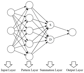 |
|
Back-Propagation Neural Network |
|
Extreme Learning Machine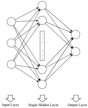 |
|
| Hybridization Techniques | Variations | Principle | Application |
|---|---|---|---|
| Averaging | Simple Averaging | Treat each and every artificial intelligence models as equally good models by obtaining their output mean value | Suitable for less complex problems where outputs of several models can be averaged directly |
| Weighted Averaging | Assign weights to each artificial intelligence models based on certain performance measure prior averaging their results | ||
| Simple Taylor Skill | Weights assigned to each artificial intelligence models are derived by considering more than one performance measures | ||
| Bootstrap Aggregating | Bags of samples are created from original sample (“apparent population”) so that more than one model can be trained and the results are aggregated | Suitable when original sample size is too small or results have high variance and bias | |
| Bayesian Modelling Approaches | Bayesian Model Averaging; Bayesian Model Selection | Weights assigned to each artificial intelligence models are computed based on the posterior probabilities given that the model accurately explain the problems | Can be used to assess the suitability or ability of a model to describe a problem |
| Boosting Algorithm | Gradient Boosting; Extreme Gradient; Boosting; Light Gradient Boosting | Combine several weak learners (poor performing artificial intelligence models) to form a strong model | Suitable to be used when there are numerous weak learners of different aspects are available |
| Nonlinear Neural Ensemble | Feed the output of several models into a secondary ANN and rely on black-box operation to obtain the ensemble | Shall be the last resort when no other more intuitive hybridization method is suitable to create an ensemble | |
| Data Decomposition | Wavelet Decomposition; Multivariate Empirical Mode Decomposition; Tensor Decomposition | De-noise the time series data to obtain the trends of different temporal resolutions in order to forecast the future trends | Can be used when time series data are available and when there is a need of forecasting future events |
| STARFM | Learn using satellite image pairs to compute predictions based on only one image | For remote sensing data application | |
| ESTARFM | Improvement on STARFM in order to handle images with non-uniform pixels or resolutions | For remote sensing data application | |
| Kalman Filter Based Ensemble | Estimate state model by only using observable model as input | Can be used when there are clear definitions of observable and state models |
| Base Model | Artificial Neural Network | Support Vector Machine | Tree Based Model | Fuzzy Logic | |
|---|---|---|---|---|---|
| Hybridization Technique | |||||
| Averaging | √ 1 | √ | √ | √ | |
| Bootstrap Aggregating | √ | SVM does not require much data to map the relationship. Instead, it needs good support vector (data) to infer the relationship between inputs and outputs. Therefore, bootstrap aggregating is seldom used for in SVM hybrid models. | √ | Fuzzy model itself contains rules that is interpretable by human language. Researchers tend to apply black-box based hybridization method on it. | |
| Bayesian Model Averaging | √ | √ | √ | ||
| Boosting Algorithm | Boosting algorithm is not necessary for ANN as ANN itself is powerful enough to map most of the relationships (not weak learner). | SVM is also a strong learner and therefore the application of boosting algorithm on it is unnecessary. | √ | ||
| Data Decomposition | √ | √ | √ | ||
| Nonlinear Neural Ensemble | √ | √ | Flexibility of tree based model allows multiple hybridization techniques to be used. It is believed that studies which include tree based model in nonlinear neural ensemble will be available in the future. | √ | |
© 2020 by the authors. Licensee MDPI, Basel, Switzerland. This article is an open access article distributed under the terms and conditions of the Creative Commons Attribution (CC BY) license (http://creativecommons.org/licenses/by/4.0/).
Share and Cite
Chia, M.Y.; Huang, Y.F.; Koo, C.H.; Fung, K.F. Recent Advances in Evapotranspiration Estimation Using Artificial Intelligence Approaches with a Focus on Hybridization Techniques—A Review. Agronomy 2020, 10, 101. https://doi.org/10.3390/agronomy10010101
Chia MY, Huang YF, Koo CH, Fung KF. Recent Advances in Evapotranspiration Estimation Using Artificial Intelligence Approaches with a Focus on Hybridization Techniques—A Review. Agronomy. 2020; 10(1):101. https://doi.org/10.3390/agronomy10010101
Chicago/Turabian StyleChia, Min Yan, Yuk Feng Huang, Chai Hoon Koo, and Kit Fai Fung. 2020. "Recent Advances in Evapotranspiration Estimation Using Artificial Intelligence Approaches with a Focus on Hybridization Techniques—A Review" Agronomy 10, no. 1: 101. https://doi.org/10.3390/agronomy10010101