A Review of Current and Potential Applications of Remote Sensing to Study the Water Status of Horticultural Crops


School of Agriculture, Food and Wine, The University of Adelaide, PMB 1, Glen Osmond, SA 5064, Australia
*
Author to whom correspondence should be addressed.
Agronomy 2020, 10(1), 140; https://doi.org/10.3390/agronomy10010140
Submission received: 25 August 2019
/
Revised: 10 December 2019
/
Accepted: 9 January 2020
/
Published: 17 January 2020
(This article belongs to the Special Issue Increasing Agricultural Water Productivity in a Changing Environment)
Abstract
:With increasingly advanced remote sensing systems, more accurate retrievals of crop water status are being made at the individual crop level to aid in precision irrigation. This paper summarises the use of remote sensing for the estimation of water status in horticultural crops. The remote measurements of the water potential, soil moisture, evapotranspiration, canopy 3D structure, and vigour for water status estimation are presented in this comprehensive review. These parameters directly or indirectly provide estimates of crop water status, which is critically important for irrigation management in farms. The review is organised into four main sections: (i) remote sensing platforms; (ii) the remote sensor suite; (iii) techniques adopted for horticultural applications and indicators of water status; and, (iv) case studies of the use of remote sensing in horticultural crops. Finally, the authors’ view is presented with regard to future prospects and research gaps in the estimation of the crop water status for precision irrigation.
1. Introduction
Understanding the water status of crops is important for optimal management and application of water to accommodate for inter and intra-field variability to achieve a specific target, such as maximum water use efficiency, yield, quality, or profitability [1,2]. The importance of optimal water management in agriculture in semi-arid or arid regions has become increasingly important in light of recent water scarcities through reduced allocations, as well as increased demand due to greater areas under production [3,4]. Climate change is expected to further intensify the situation due to the increased frequency of heatwaves and drought episodes [5]. Climate change coupled with the necessity to increase food production due to an increase in global population has placed pressure on horticultural sector to improve efficiencies in resources use, e.g., water, for sustainable farming [6,7,8,9,10]. Horticultural crops will have to produce more ‘crop-per-drop’ in the face of limited water resources. Informed management of water resources whilst maintaining or increasing crop quality and yield are the primary goals of irrigation scheduling in horticulture. These goals can be achieved by improving our understanding of the water status of the crops at key phenological stages of development.
Traditional decision-making for irrigation of horticultural crops includes using information from a combination of sources such as historical regimes, soil moisture measurements, visual assessments of soil and/or crop, weather data including evapotranspiration (ET), and measurements of crop water status using direct-, proximal- or remote-sensing techniques [11,12,13]. Some growers undertake routine ground-based measurements, e.g., pressure chamber, for estimation of crop water status to make decisions on irrigation [14,15,16]. These ground-based measurements are robust; however, destructive, cumbersome, and expensive to acquire a reasonable amount of data [14,16,17,18]. Consequently, the measured leaf is assumed to represent the average population of leaves of the individual crop, and a few crops are assumed to represent the average population of the entire irrigation block. As a result, over- or under-watering can occur, which can lower yield and fruit quality [19,20,21,22]. This is especially evident for non-homogenous blocks where spatial variability of soil and water status is expected [23,24,25].
To address some of the limitations of ground-based measurements, remote measurement techniques were introduced with capabilities to measure at higher spatial resolution, larger area, and on a regular basis [26,27,28,29]. Remote sensing, in particular, unmanned aircraft systems (UAS), presents a flexible platform to deploy on-demand sensors as a tool to efficiently and non-destructively measure crop water status [30]. Using thermal and spectral signatures, remote sensing techniques can be used to characterise a crop’s water status. Knowledge of crop water status allows growers to more efficiently schedule irrigation (i.e., when and how much water to apply). In this regard, UAS platforms provide a convenient methodology to monitor the water status across a farm, both spatially and temporally at the canopy level [31,32,33]. The spectral, spatial, and temporal flexibility offered by UAS-based remote sensing may in future assist growers in irrigation decision-making [34,35].
This review provides an overview of the application of remote sensing to understand the crop’s water status (e.g., leaf/stem water potential, leaf/canopy conductance), soil moisture, ET, and physiological attributes, all of which can contribute to understanding the crop’s water status to implement precision irrigation. Although the key focus of this review is UAS-based remote sensing, a comparison has been undertaken with other remote sensing platforms, such as earth observation satellites, which are being increasingly used to acquire similar information. In the following sections, we provide an overview of the most common remote sensing platforms in horticulture, various sensors used for remote sensing, and several predictive indices of crop water status. Two case studies of remote sensing in horticultural crops, grapevine and almond, are then presented followed by an overview of the current research gaps and future prospects.
2. Remote Sensing Platforms
Ground-based direct or proximal sensors acquire instantaneous water status measurement from a spatial location. For decision-making purposes, the data is generally collected from multiple locations across a field, which allows geospatial interpolation, such as kriging, to be applied [36,37,38]. This scale of data collection is, however, cumbersome, inefficient, and error-prone, especially for water status measurements of large areas [17]. Monitoring and observing farms at a larger spatial scale prompted the launch of several earth observation satellite systems that typically operate at an altitude of 180–2000 km [39]. Manned high-altitude aircraft (operating within few km) and, more recently, UAS (operating under 120 m) filled the spatial gap between high-resolution ground measurements and relatively low-resolution satellite measurements [40,41]. In the context of water status estimation for horticultural crops, all the aforementioned remote sensing platforms are utilised depending on the user requirements [23,42,43]. Each remote sensing platform has its own advantage and shortcomings. The decision to obtain remote sensing crop water status data from one or more of these platforms will depend on the spatial and temporal resolution desired. Satellite and manned aircraft can be useful for regional-scale characterisation, whereas UAS can be more useful to map the intra-field variability. Vehicle-based ground systems also possess similar measurement capabilities, like remote sensing, however, at a smaller scale [44,45]. These systems can move within the horticultural rows obtaining water status measurements of adjacent plants while the vehicle is moving, enabling them to cover a relatively larger area as compared to ground-based direct measurements [46,47,48].
2.1. Satellite Systems
The use of satellite systems for remote sensing started with the launch of Landsat-1 in 1972 [39,49]. The subsequent launch of SPOT-1 in 1986 and Ikonos in 1999 opened the era of commercial satellite systems that resulted in rapid improvement in imaging performance, including spatial and spectral resolution [50]. Continued launch of satellites from the same families, with newer sensor models and improved capability, resulted in the formation of satellite constellations (e.g., Landsat, Sentinel, SPOT, RapidEye, GeoEye/WorldView families). The satellite constellation substantially improved the revisit cycle of the satellite system [51]. Recently, the miniature form of the satellite termed Nanosat or Cubesat has been developed, which can be deployed on the same orbit in a large number (20s–100s), enabling frequent and high-resolution data acquisition (e.g., Dove satellite from Planet Labs) [52].
The earth observation satellite system, such as Landsat, Sentinel, MODIS, RapidEye, and GeoEye, have been used to study horticultural crops (Table 1). These satellite system offer camera systems with spectral bands readily available in visible, near infrared (NIR), short-wave infrared (SWIR), and thermal infrared (TIR). The measurement in these bands provides opportunities to study a crop’s water status indirectly via, for example, calculation of the normalised difference vegetation index (NDVI), crop water stress index (CWSI), and ET [8,9,10] at the field- and regional-scales.
The reflected/emitted electromagnetic energy from the crop reaching the sensor is recorded at a specific wavelength. The width of the observed wavelength expressed in full width at half maximum (FWHM) is called spectral resolution. The number of observed bands and the spectral resolution indicates the ability of the satellite to resolve spectral features on the earth’s surface. Commonly used earth observation satellite systems possess between four and 15 bands with approximately 20–200 nm FWHM spectral resolution. The bands are generally designated for the visible and NIR region with extended capabilities in SWIR, TIR, as well as red edge region (Table 1). The most widely used band combinations to study the water status of vegetation are the visible, NIR and TIR bands [23,25,53,54]. With the plethora of satellite systems currently available, user requirements on band combination may be achieved by using multiple satellites. However, acquiring an extra or a narrower band to the existing capabilities is not possible.
The ground distance covered per pixel of the satellite image is called the spatial resolution, whereby, a higher spatial resolution indicates a smaller ground distance. Existing satellite systems, due to their lower spatial resolution and large coverage, are suited to study larger regions [55]. For a smaller observation area, such as a farm block, an irrigation zone, a single row of the horticultural crop, or a single canopy, this spatial resolution is considered sub-optimal. Often, a pixel of the satellite image comprises of multiple rows and multiple canopies of horticultural crops [42,56]. Thus, the spectral response on a single pixel of the satellite image includes a mixed spectral signal from the canopy, inter-row vegetation and/or bare soil. The mixed-pixel is particularly unavoidable in horticultural crops with large inter-row surfaces, introducing errors in satellite-based estimations [42,56]. Improving the spatial resolution from freely available Landsat/Sentinel satellites (spatial resolution 10–15 m) to such as WorldView-3 (spatial resolution 0.3 m), does not necessarily resolve single canopies of many horticultural crops.
Current satellite systems generally offer a temporal resolution of about 1–2 weeks this resolution corresponds to the satellite’s revisit interval (Table 1). For example, freely available Landsat-8 and Sentinel-2 offer revisit cycles of 16 and 5 days, respectively. Although the MODIS sensor on NASA’s Terra and Aqua satellites offer a greater temporal resolution (1–2 days), its spatial resolution is relatively coarse (250 m–1 km) to be valuable for horticulture [25]. The revisit cycle of satellites does not alone represent the timeframe on which the data can be interpreted. For instance, post-data acquisition, there are often delays in data transfer to the ground station, handling, and delivery to the end user. The end user then needs to process the data before making an interpretation. Such processing can be a combination of atmospheric, radiometric, and geometric corrections, where applicable [57,58]. Furthermore, as the agricultural applications of the satellite imagery are illumination sensitive and weather dependent, conditions have to be optimal on the satellite revisit day to avoid data corruption due to, for example, cloud cover [23,53]. Cloud corrupted data (~55% of the land area is covered by cloud at any one time [59]) will require users to wait for the next revisit to attempt the data acquisition. Time-series image fusion techniques, such as the spatial and temporal adaptive reflectance fusion model, can improve the spatial and temporal resolution of the satellite data [60,61]. These fusion techniques blend the frequent (however low-resolution) with higher-resolution (but infrequent) satellite data [62,63]. The result combines the best aspects of multiple satellite systems to produce frequent and higher-resolution data, which can be useful for timely monitoring of water status.
The clear advantage of the satellite system is the ability to capture data at a large scale and at an affordable cost (e.g., the user can download Landsat and Sentinel data for free). The compromise with the satellite data is in spatial resolution, as well as the relatively long revisit cycle (in the order of days to weeks), making the data less than ideal for specific applications, e.g., irrigation scheduling.
2.2. Manned Aircraft System
Operating within few kilometres above ground level, manned aircraft have been used to remotely acquire agricultural data at higher spatial detail (compared to the satellites) and over a larger region (compared to UAS) [42,64]. Light fixed-wing aircraft and helicopters are the commonly used manned aircraft employed in agricultural remote sensing. The fixed-wing aircraft generally flies higher and faster, enabling the coverage of a larger area, whereas the helicopters are traditionally flown lower and slower, enabling a spatially detailed observation. A significant advantage of the manned aircraft, compared to UAS, lies in their ability to carry heavier high-grade sensors, such as AVIRIS, HyPlant, HySpex SWIR-384, Specim AisaFENIX, and Riegl LMS Q240i-60 [65,66,67]. The use of manned aircraft is, however, limited by high operational complexity, safety regulations, scheduling inflexibility, costs, and product turnaround time. As a result, these platforms are barely used as compared to the recent surge in the use of UAS, specifically for horticultural crops [68,69,70].
In horticulture, manned aircraft was used to characterise olive and peach canopy temperature and water stress using specific thermal bands (10.069 µm and 12.347 µm) of a wideband (0.43–12.5 µm) airborne hyperspectral camera system [71,72]. This work found moderate correlations (R2 = 0.45–0.57) of ground vs. aerial olive canopy temperature measurements [72], and high correlations (R2 = 0.94) of canopy temperature vs. peach fruit size (diameter) [71]. The advantage of manned aircraft for remote sensing of a large region was highlighted in recent work that characterised regional-scale grapevine (Vitis vinifera L.) water stress responses of two cultivars, Shiraz and Cabernet Sauvignon, in Australia [64]. Airborne thermal imaging was able to discriminate between the two cultivars based on their water status responses to soil moisture availability (Figure 1).
2.3. Unmanned Aircraft Systems
Both the fixed-wing and the rotary-wing variant of UASs are used in agricultural remote sensing. Each variant has its advantages and shortcomings vis-à-vis sensor payload, flexibility, and coverage. In this regard, the literature provides a list of state-of-the-art UAS [73], their categorisation [74], and overview of structural characteristics, as well as flight parameters [75], in the context of agricultural use. Depending on the number of rotors, a rotary-wing UAS can be a helicopter, a quadcopter, a hexacopter, or an octocopter, among others. Rotary-wing UAS are more agile and can fly with a higher degree of freedom [76], while fixed-wing UAS needs to be moving forward at a certain speed to maintain thrust. As a result, rotary-wing UAS provides flexibility and specific capabilities, such as hovering, vertical take-off and landing, vertical (up and down) motions, or return to the previous location. On the contrary, fixed-wing UAS fly faster, carry heavier payloads, and have greater flying time enabling coverage of larger areas in a single flight [77]. Recently developed fixed-wing UAS with vertical take-off and landing capabilities, such as BirdEyeView FireFly6 PRO, Elipse VTOL-PPK, and Carbonix Volanti, captures the pros of both fixed-wing and rotary-wing, making them a promising platform for agricultural purposes. In the context of precision agriculture, the application of UAS, their future prospects, and knowledge gaps are discussed in [53,78,79,80,81]. While many horticultural crops have been studied using UAS technology, the most studied horticultural crops are vineyards [31,82,83,84], citrus [85,86], peach [32,33], olive [18,87,88], pistachio [89,90], and almond [91,92,93,94], among others [95,96,97,98,99]. Some of the UAS types used for water status studies of horticultural crops are shown in Figure 2.
UAS offers flexibility on spatial resolution, observation scale, spectral bands, and temporal resolution to collect data on any good weather day. However, like satellite and manned aircraft, the UAS is inoperable during precipitation, high winds, and temperatures. By easily altering the flying altitude, the UAS provides higher flexibility to observe a larger area with lower spatial resolution or smaller area with much greater detail [103]. Temporally, the UAS can be scheduled at a user-defined time at short notice, thus accommodating applications that are time-sensitive, such as capturing vital phenological stages of crop growth. Spectrally, UAS offer flexibility to carry on-demand sensors and interchangeability between sensor payloads; thus, any desired combination of sensors and spectral bands can be incorporated to target specific features.
UAS-acquired image data requires post-processing before it can be incorporated into the grower decision-making process. Mosaicking of UAS images currently has a turnaround time of approximately one day to one week, subject to the size of the dataset, computational power, and spectral/spatial quality of the product [104,105]. Spectral quality of the data is of optimal importance, whereas the spatial quality can be of less importance, such as for well-established horticultural crops. Higher spectral quality demands calibration of the spectral sensors and correction of atmospheric effects. Following post-processing of aerial images, the UAS-based spectral data have shown to be highly correlated with ground-based data [82,102,106].
The most common UAS-based sensor types to study the crop water status are the thermal, multispectral and RGB, while hyperspectral and LiDAR (Light detection and ranging) sensors are used less often [23,79,107]. Spectral sensors provide the capability to capture broader physiological properties of the crop, such as greenness (related to leaf chlorophyll content and health) and biomass, that generally correlate with crop water status [82,108]. Narrower band spectral sensors provide direct insight into specific biophysical and biochemical properties of crops, such as via photochemical reflectance index (PRI) and solar-induced chlorophyll fluorescence (SIF), which reflects a plant’s photosynthetic efficiency [109,110]. Thermal-based sensors capture the temperature of the crop’s surface, which indicates the plant’s stress (both biotic and abiotic) [53]. Generally, digital RGB camera and LiDAR can be used to quantify 3D metrics, such as the plant size and shape, via 3D pointclouds with sufficient accuracy for canopy level assessment [111,112,113,114,115,116,117,118].
3. Remote Sensor Types
3.1. Digital Camera
A digital camera typically incorporates an RGB, modified RGB, and a monochrome digital camera. The lens quality of the camera determines the sharpness of the image, while the resolution of the camera determines its spatial resolution and details within an image. The RGB camera uses broad spectral bandwidth within the blue, green and red spectral region to capture energy received at the visible region of the electromagnetic spectrum. The images are used to retrieve dimensional properties of the crop, terrain configuration, macrostructure of the field, and the spatial information. Based on the dimensional properties, such as size, height, perimeter, and area of the crown, the resource need practices can be estimated [119,120,121]. Generally, a larger crop is expected to more quickly use available water resources, resulting in crop water stress at a later stage of the season if irrigation is not sufficient. The evolution of canopy structure within and between seasons can be useful to understand the spatial variability within the field and corresponding water requirements. The macro-structure of horticultural crops, such as row height, width, spacing, crop count, the fraction of ground cover, and missing plants, can be identified remotely, which can aid in the allocation of resources [113,122]. The terrain configuration in the form of a digital elevation model (DEM) generated from a digital camera can also enable understanding of the water status in relation to the aspect and slope configuration of the terrain.
3.2. Multispectral Camera
A multispectral camera offers multiple spectral bands across the electromagnetic spectrum. Most common airborne multispectral cameras have 4–5 bands which include rededge and NIR bands in addition to the visible bands, R-G-B (e.g., Figure 3a,c). Configurable filter placement of the spectral band is also available, which can potentially target certain physiological responses of horticultural crops [102]. Spectrally, the airborne multispectral camera has been reported to perform with consistency, producing reliable measurements following radiometric calibration and atmospheric correction [123,124,125]. Their spatial resolution has been found to be sufficient for horticultural applications enabling canopy level observation of the spectral response. For this reason, as well as relatively low cost, multispectral cameras are used more frequently in horticulture applications.
Chlorophyll and cellular structures of vegetation absorb most of the visible light and reflect infrared light. The rise in reflectance between the red and NIR band is unique to live green vegetation and is captured by vegetation spectral index called NDVI (Table 2, Equation (3)). Once the vegetation starts to experience stress (biotic and abiotic), its reflectance in the NIR region is reduced, while the reflectance in the red band is increased. Thus, such stress is reflected in the vegetation profile and easily captured by indices, such as NDVI. For this reason, NDVI has shown correlations with a wide array of crops response including vigour, chlorophyll content, leaf area index (LAI), crop water stress, and occasionally yield [34,82,83,84,127].
The rededge band covers the portion of the electromagnetic spectrum between the red and NIR bands where reflectance increases drastically. Studies have suggested that the sharp transition between the red absorbance and NIR reflection is able to provide additional information about vegetation and its hydric characteristics [128]. Using the normalised difference red edge (NDRE) index, the rededge band was found to be useful in establishing a relative chlorophyll concentration map [127]. Given the sensitivity of NDRE, it can be used for applications, such as crops drought stress [107]. With regard to the water use efficiency, a combination of vegetation indices (VIs) along with structural physiological indices were found to be useful to study water stress in horticultural crops [34,82,129].
3.3. Hyperspectral
Hyperspectral sensors have contiguous spectral bands sampled at a narrower wavelength intervals spanning from visible to NIR spectrum at a high to ultra-high spectral resolution (Figure 3d). Scanning at contiguous narrow-band wavelengths, a hyperspectral sensor produces a three dimensional (two spatial dimensions and one spectral dimension) data called hyperspectral data cube. The hyperspectral data cube is a hyperspectral image where each pixel contain spatial information, as well as the entire spectral reflectance curve [130]. Based on the operating principle and output data cube, hyperspectral sensors for remote sensing can include a point spectrometer (aka spectroradiometer), whiskbroom scanner, pushbroom scanner, and 2D imager (Figure 4) [130,131]. A point spectrometer, samples within its field of view solid angle to produce an ultra-high spectral resolution spectral data of a point [130,132]. A whiskbroom scanner deploys a single detector onboard to scan one single pixel at a time. As the scanner rotates across-track, successive scans form a row of the data cube, and as the platform moves forward along-track, successive rows form a hyperspectral image [133]. A pushbroom scanner deploys a row of spatially contiguous detectors arranged in the perpendicular direction of travel and scans the entire row of pixels at a time. As the platform moves forward, the successive rows form a two-dimensional hyperspectral image [40,134]. The 2D imager using different scanning techniques [130] captures hyperspectral data across the image scene [135,136]. The point spectrometer offers the highest spectral resolution and lowest signal-to-noise ratio (SNR) among the UAS-compatible hyperspectral sensors [137,138].
In horticultural applications, hyperspectral data, due to the high resolution contiguous spectral sampling, possesses tremendous potential to detect and monitor specific biotic and abiotic stresses [139]. Narrowband hyperspectral data was used to detect water stress using the measurement of fluorescence and PRI over a citrus orchard [110]. PRI was identified as one of the best predictors of water stress for a vineyard in a study that investigated numerous VIs using hyperspectral imaging [140]. High-resolution thermal imagery obtained from a hyperspectral scanner was used to map canopy stomatal conductance (gs) and CWSI of olive orchards where different irrigation treatments were applied [18]. With the large volume of spatial/spectral data extracted from the hyperspectral data cube, machine learning will likely be adopted more widely in the horticultural environment to model water stress [141]. See Reference [54] for a comprehensive review of hyperspectral and thermal remote sensing to detect plant water status.
3.4. Thermal
Thermal cameras use microbolometers to read passive thermal signals in the spectral range of approximately 7–14 µm (Figure 3b). Small UAS are capable of carrying a small form-factor thermal camera with uncooled microbolometers, which does not use an internal cooling mechanism and, therefore, does not achieve the high SNR that can be found in cooled microbolometer-based thermal cameras. An array of microbolometer detectors in the thermal camera receives a thermal radiation signal and stores the signal on the corresponding image pixel as raw data number (DN) values. The result is a thermal image where each pixel has an associated DN value, which can be converted to absolute temperature. A representative list of commercial thermal cameras used on UAS platforms and their applications with regard to agricultural remote sensing is found in the literature [23,53,73]. Thermal imagery enables the measurement of the foliar temperature of plants. The foliar temperature difference between well-watered and water-stressed crops is the primary source of information for water stress prediction using a thermal sensor [142]. When mounted on a remote sensing platform, the canopy level assessment of crop water status can be performed on a large scale.
Thermal cameras are limited by their resolution (e.g., 640 × 512 is the maximum resolution of UAS compatible thermal cameras in the current market) and high price-tag [53]. The small number of pixels results in low spatial resolution limiting either the ability to resolve a single canopy or ability to fly higher and cover a larger area. If flown at a higher altitude, the effective spatial resolution may be inadequate for canopy level assessment of some horticultural crops. For example, a FLIR Tau2 640 thermal camera with a 13 mm focal length when flown at an altitude of approximately 120 m results in a spatial resolution of 15.7 cm. For relatively large horticultural crops, such as grapevine, almond, citrus, and avocado, the resolution at a maximum legal flying altitude of 120 m in Australia (for small-sized UAS) offers an adequate spatial resolution to observe a single canopy.
Another challenge with the use of thermal cameras is the temporal drift of the DN values within successive thermal images, especially with uncooled thermal cameras [143]. Due to the lack of an internal cooling mechanism for the microbolometer detectors, DN values registered by the microbolometers experience temporal drift i.e., the registered DN values for the same temperature target will drift temporally. Thus, the thermal image can be unreliable especially when the internal temperature of the camera is changing rapidly, such as during camera warmup period or during the flight when a gust of cool wind results in cooling of the camera. To overcome this challenge, the user may need to provide sufficient startup time before operation (preferably 30–60 min) [102,143,144,145], shield the camera to minimize the change in the internal temperature of the camera [142], calibrate the camera [146,147,148,149,150,151,152,153], and perform frequent flat-field corrections.
3.5. Multi-Sensor
To carry multiple sensors, the total UAS payload needs to be considered that includes, in addition to the sensors, an inertial measurement unit (IMU) and global navigation satellite system (GNSS) for the georeferencing purpose [40,154]. Higher accuracy sensors tend to be heavier, and in a multi-sensor scenario, the payload can quickly reach or even exceed the payload limit. This has limited contemporary measurements in earlier multirotor UAS requiring separate flights for each of sensor [126]. The use of fixed-wing UAS has allowed carrying higher payloads due to the much larger thrust-to-weight ratio as compared to a rotary-wing aircraft [155]. Similarly, recent advancement in UAS technology and lightweight sensors have enabled multirotor (payload 5–6 kg readily available) to onboard multi-sensors.
Water status of crops is a complex process influenced by a number of factors including the physiology of the crop, available soil moisture, the size and vigour of the crop, and meteorological factors [30,108,116,156,157]. For this reason, a multi-sensor platform is used to acquire measurements of the different aspects of the crop for water status assessment [34,102,108]. The most common combination of sensors found in the literature is the RGB, multispectral (including rededge and NIR bands) and thermal. Together, these sensors can be used to investigate the water status of the crop using various indicators, such as PRI, CWSI, fluorescence, and structural properties, with the aim of improving the water use efficiency [102,110,158,159,160].
4. Techniques of Remote Sensing in Horticulture
4.1. Georeferencing of Remotely Sensed Images
Georeferencing provides a spatial reference to the remotely sensed images such that the pixels representing crops or regions of interest on the images are correctly associated with their position on Earth. The georeferencing process generally uses surveyed coordinate points on the ground, known as ground control points (GCPs), to determine and apply scaling and transformation to the aerial images [161]. Alternatively, instead of GCPs, the user can georeference aerial images by using the accurate position of the camera, or by co-registration with the existing georeferenced map [105,162].
In the case of UAS-based images, the capture timing is scheduled to ensure a recommended forward overlap (>80%) between successive images. The flight path is designed to ensure the recommended side overlap (>70%) between images from successive flight strips. Thus, the captured series of images are processed using the Structure-from-Motion (SfM) technique to generate a 3D pointcloud and orthomosaic [73,130] (see Figure 5). Commonly used SfM software to process the remote sensing images are Agisoft PhotoScan and Pix4D. The commonly retrieved outputs from the SfM software for assessment of horticulture crops include the orthomosaic, digital surface model (DSM), DEM, and 3D pointcloud [113,126,163]. This technique of georeferencing can be applied to any sensor that produces images, e.g., RGB, thermal, or multispectral cameras [126,164,165].
The complexity of georeferencing of hyperspectral observations depends on the sensor type, i.e., imaging or non-imaging. A non-imaging spectroradiometer relies on the use of a GNSS antenna and an IMU for georeferencing the point observation [130,132,138,168]. An imaging hyperspectral camera, generally, in addition to GNSS and IMU measurement, uses the inter-pixel relation in SfM to produce a georeferenced orthomosaic [40,134,135,169,170].
4.2. Calibration and Correction of Remotely Sensed Images
Ensuring consistency, repeatability, and quality of the spectral observation requires stringent radiometric, spectral, and atmospheric corrections [123,171,172,173,174,175,176,177]. Spectral and radiometric calibration is performed in the spectral calibration facility in darkroom settings. The sensor’s optical properties and shift in spectral band position are corrected during the spectral calibration process. Radiometric calibration enables conversion of the recorded digital values into physical units, such as radiance. Infield operation of the spectral sensor is influenced by variations in atmospheric transmittance from thin clouds, invisible to the human observer. Changes in atmospheric transmittance affect the radiance incident on the plant. As a result, the change in acquired spectral response by the sensor may not represent the change in plants response but the change in incident radiation on the plant. The most common method to convert the spectral data to reflectance is by generating an empirical line relationship between sensor values and spectral targets, such as a Spectralon® or calibration targets. The use of downwelling sensors, such as a cosine corrector [137], or the use of a ground-based PAR sensor enables absolute radiometric calibration to generate radiance [130].
The calibration of the broad wavelength multispectral sensor is generally less stringent than the hyperspectral. Generally, multispectral sensors are used to compute normalised indices such as NDVI. The normalised indices are relatively less influenced, although significant, by the change in illumination conditions which affect the entire spectrum proportionally [29,101]. In this regard, radiometric calibration of the multispectral camera has used a range of stringent to simplified, and vicarious approaches [123,125,171,173,178,179,180]. Some multispectral cameras are equipped with a downwelling light sensor, which is aimed at correcting for variations in atmospheric transmittance. However, the performance of such downwelling sensors (without a cosine corrector) on multispectral cameras have been reported to have directional variation resulting in unstable correction, indicating the inability of the sensor to incorporate the entire hemisphere of diffused light [124,137].
The radiometric calibration of the thermal images is typically based on the camera’s DN to object temperature curve, which provides the relationship between the DN of a pixel and a known object temperature, usually of a black body radiator. Measurement accuracy and SNR of the camera under varying ambient temperatures can be improved by using calibration shutters, which are recently available commercially. Furthermore, for low measurement errors (under 1 °C), thermal data requires consideration to the atmospheric transmittance [18,102]. Flying over a few temperature reference targets placed on the ground reduces the temporal drift of the camera [142,143,181]. Temperature accuracy within a few degrees was achieved by flying over the targets three times (at the start, middle and end of UAS operation) and using three separate calibration equations for each overpass [142]. Additionally, using the redundant information from multiple overlapping images, drift correction models have been proposed, which lowered temperature error by 1 °C as compared to uncorrected orthomosaic [152]. The manufacturer stated accuracies (generally ±5 °C) can be sufficient to access the field variability and to detect “hotspots” of water status. However, the aforementioned calibration and correction of the thermal cameras are required for quantitative measurement as a goal [143]. In this regard, current challenges and best practices for the operation of thermal cameras onboard a UAS is provided in the literature [143].
4.3. Canopy Data Extraction
A key challenge in remote sensing of horticultural as compared to agricultural crops arises due to the proportion of inter-row ground/vegetation cover and resulting mixed pixels. The proportion of the mixed pixels increases with the decrease in spatial resolution of the image. Most of the pixels towards the edge of the canopy contain a blend of information originating from the sun-lit canopy, shadowed leaves, and inter-row bare soil/cover crop. A further challenge can arise for some crops, such as grapevine, due to overlapping of adjacent plants.
The canopy data from orthomosaic has been extracted using either a pixel-based or an object-based approach. Earlier studies manually sampled from the centre of crop row which most likely eliminated the mixed pixels [182]. In the pixel-based approach, techniques, such as applying global threshold and masking, have been used. Binary masks, such as NDVI, eliminates non-canopy pixels from the sampling [82,84]. Combining the NDVI mask with the canopy height mask can exclude the pixels associated with non-vegetation, as well as vegetation that does not meet the height threshold. The pixel-based approach, however, can result in inaccurate identification of some crops due to pixel heterogeneity, mixed pixels, spectral similarity, and crop pattern variability.
In the object-based approach, using object detection techniques, neighbouring pixels with homogenous information, such as spectral, textural, structural, and hierarchical features, are grouped into “objects”. These objects are used as the basis of object-based image analysis (OBIA) classification using classifiers, such as k-nearest neighbour, decision tree, support vector machine, random forest, and maximum likelihood [122,183,184,185]. In the horticultural environment, OBIA has been adopted to classify and sample from pure canopy pixels [119,122,186]. Consideration should be provided on the number of features and their suitability for a specific application to reduce the computational burden, as well as to maintain the accuracies. The generalisation of these algorithms for transferability between study sites usually penalises the achievable accuracy. For details in object-based approach of segmentation and classification, readers are directed to literatures [122,183,185,187,188,189].
Other techniques found in the literature include algorithms, such as ‘Watershed’, which has been demonstrated in palm orchards [82,190]. Vine rows and plants have been isolated and classified using image processing techniques, such as clustering and skeletisation [188,191,192,193]. Similarly, the gridded polygon, available in common GIS software, such as ArcGIS and QGIS, can be used in combination with zonal statistics for this purpose. When working with the low-resolution images, co-registration with the high-resolution images has been proposed, whereby, the high-resolution images enable better delineation of the mixed pixels [194]. For this reason, spectral and thermal sensors, which are usually low in resolution, are generally employed along with high-resolution digital cameras.
4.4. Indicators of Crop Water Status
A crop’s biophysical and biochemical attributes can be approximated using different indices and quantitative products. For example, CWSI is used to proxy leaf water potential (Ψleaf), stem water potential (Ψstem), gs, and net photosynthesis (Pn) [83,100,195]. With regard to horticultural crops, water status has been assessed using a number of spectral and thermal indices (Table 2).
4.4.1. Canopy Temperature
A plant maintains its temperature by transpiring through the stomata to balance the energy fluxes in and out of the canopy. As the plant experience stress (both biotic and abiotic), the rate of transpiration decreases, which results in higher canopy temperature (Tc), which can be a proxy to understand the water stress in the plant [207]. In this regard, crop water stress showed a correlation with canopy temperature extracted from the thermal image [208], which enables mapping the spatial variability in water status [209]. Leaf/canopy temperature alone, however, does not provide a complete characterisation of crop water status, for instance, an equally stressed canopy can be 25 °C or 35 °C, depending on the current ambient temperature (Ta). Thus, canopy-to-air temperature difference (Tc − Ta) was proposed, which showed a good correlation with the Ψstem, Ψleaf, and gs in horticultural crops [85,99,182].
4.4.2. Normalised Thermal Indices
The CWSI, the conductance index (Ig) and the stomatal conductance index (I3) are thermal indices most commonly used to estimate crop water status and gs [210,211,212]. These indices provide similar information, however, use a different range of numbers to represent the level of water stress. The CWSI is normalised within zero and one, whereas Ig and I3 represent stress using numbers between zero and infinity. CWSI has been adopted most widely in horticultural applications to assess the water status of crops, such as the grapevines [100,213], almond [91,198], citrus [85,110], and others [18,87,99,214]. By normalising between the lower and upper limits of (Tc − Ta), the CWSI of the canopy presents quantifiable relative water stress. The formula for CWSI computation is defined as in Equation (1) [208,212].
where and represent the upper and lower bound of (Tc − Ta) which are found in the water-stressed canopy and well-watered canopy transpiring at the full potential (or maximum) rate, respectively. Assuming a constant ambient temperature, Equation (1) can be simplified to Equation (2), which is the most widely reported formulation of CWSI with regard to the horticultural remote sensing.
where Twet is the temperature of canopy transpiring at the maximum potential, and Tdry is the temperature of the non-transpiring canopy. CWSI has been shown to be well-correlated with direct measurements of crop water status in the horticultural environment [18,31,32,90,99]. In this regard, a correlation of CWSI with various ground measurements, such as Ψleaf [18,31,197], Ψstem [33,90,194], and gs [18,90,100], have been established. Diurnal measurements of CWSI compared with Ψleaf showed the best correlation at noon [89,197,209].
CWSI is a normalised index, i.e., relative to a reference temperature range between Twet and Tdry, which is specific to a region and crop type; thus, CWSI is not a universal quantitative indicator of crop water status. For instance, a CWSI of 0.5 for two different varieties of grapevines at different locations does not conclusively inform that they have equal or superior/inferior water status. Furthermore, the degree of correlation can change depending on the isohydric/anisohydric response of crop [214] where early/late stomatal closure affects the indicators of water stress [110]. Moreover, phenological stage affects the relationship between remotely sensed CWSI and water stress [197]. Thus, water stress in a different crop, at a different location and at a different phenological stage, will have a unique correlation with CWSI and, therefore, needs to be established independently.
There are multiple methods to measure the two reference temperatures, Twet and Tdry, which could result in variable CWSI values depending on the method used. The first method is to measure the two reference temperatures on the crop of interest. Tdry can be estimated by inducing stomatal closure, which is the leaf temperature approximately 30 min after applying a layer of petroleum jelly e.g., Vaseline to both sides of a leaf. This effectively blocks stomata and, therefore, impedes leaf transpiration. Twet can be estimated by measuring leaf temperature approximately 30 s after spraying water on the leaf, which emulates maximum transpiration [23,83]. The advantage of this method is that the stress levels are normalised to actual plants response, whereas the necessity to repeat the measurement for every test site after each flight can be cumbersome. In an alternative (second) approach the range can be established based on meteorological data e.g., setting Tdry to 5 °C above air temperature and Twet measured from an artificial surface. This method is also limited to local scale and presents a problem regarding the choice of material, which ideally needs to have similar to leaf emissivity, aerodynamic and optical properties [54,87]. The third method uses the actual temperature measurement range of the remote sensing image [33,97]. This method is simple to implement, however, works on the assumption that the field contains enough variability to contain a representative Twet and Tdry. Fourth, the reference temperatures can be estimated by theoretically solving for the leaf surface energy balance equations, however, are limited by the necessity to compute the canopy aerodynamic resistance [87]. Standard and robust Twet and Tdry measurements are needed to characterize CWSI with accuracy, especially for temporal analysis [85,87,211]. The level of uncertainty due to the adaptation of different approaches for Twet and Tdry determination in the instantaneous and seasonal measurements of CWSI is not known. Nonetheless, adopting a consistent approach, CWSI has been shown to be suitable for monitoring the water status and making irrigation decisions of horticultural crops [31,85].
4.4.3. Spectral Indices
Crops reflectance properties convey information about the crop, for instance, a healthier crop has higher reflectance in the NIR band. Most often, the bands are mathematically combined to form VIs, which provide information on the crop’s health, growth stage, biophysical properties, leaf biochemistry, and water stress [29,215,216,217,218]. Using multispectral or hyperspectral data, several Vis, such as green normalised difference vegetation index (GNDVI), renormalised difference vegetation index (RDVI), optimized soil-adjusted vegetation index (OSAVI), transformed chlorophyll absorption in reflectance index (TCARI), and TCARI/OSAVI, amongst others [34,79,82], can be calculated that correlate with the water stress of horticultural crops (see Table 2). The most widely studied VI in horticulture, in this regard, is the NDVI (Equation (3)).
where and represent the spectral reflectance acquired at the NIR and red spectral regions, respectively. In horticulture, NDVI has been used as a proxy to estimate the vigour, biomass, and water status of the crop. A vigorous canopy with more leaves regulates more water, therefore remaining cooler when irrigated [200] and experiencing early water stress when unirrigated. With regard to irrigation, the broadband normalised spectral indices (such as NDVI) are suitable to detect spatial variability and to identify the area that is most vulnerable to water stress. However, these indices are not expected to change rapidly to reflect the instantaneous water status of plants that are needed to make decisions on irrigation scheduling.
The multispectral indices along with complementary information in thermal wavelengths have proven to be well suited to monitoring vegetation, specifically in relation to water stress [219]. The ratio of canopy surface temperature to NDVI, defined as temperature-vegetation dryness index (TVDI), was found to be useful for the study of water status in horticultural crops. TVDI exploits the fact that vegetation with larger NDVI will have a lower surface temperature unless the vegetation is under stress. As most vegetation normally remains green after an initial bout of water stress, the TVDI is more suited than NDVI for early detection of water stress as the surface temperature can rise rapidly even during initial water stress [200].
Similarly, narrowband VIs that have been studied in relation to remote sensing of water status are PRI and chlorophyll fluorescence, which have been directly correlated to the crop Ψleaf, gs [110,182,204]. Several hyperspectral indices to estimate water status have been identified [139]; however, their application in remote sensing of horticultural crops is at its infancy. Hyperspectral indices specific to water absorption bands around 900 nm, 1200 nm, 1400 nm, and 1900 nm may be used to detect the water status of horticultural crops. The absorption features were found to be highly correlated with plant water status [139]. Water band index (WBI), as defined in Equation (4), has been shown to closely track the changes in the plant water status of various crops [202,203].
Other water-related hyperspectral indices with potential application for horticultural crops can be found in the literature [139,202,203]. Hyperspectral data possess the capability to reflect the instantaneous water status of the plant, which can be useful for quantitative decision-making on irrigation scheduling.
4.4.4. Soil Moisture
The moisture status of the soil provides an indication of the available water resource to the crop. Soil moisture is traditionally measured indirectly using soil moisture sensors placed below the surface of the soil. A key challenge with using soil moisture sensors are the spatial distribution of moisture, both vertically and horizontally, to account for inherent field-scale variability. For instance, the root system of some horticultural crops, such as grapevine, is capable of accessing water up to 30 m deep, while customer-grade soil moisture probes generally extend to 1.5 m in depth or less. Thus, soil moisture probes do not capture all the water available to the crop as they are point measures and not necessarily where the roots are located. Moreover, estimation of soil moisture across spatial and temporal scales is of interest for various agricultural and hydrological studies. Optical, thermal, and microwave remote sensing with their advantages relating to high spatial scale and temporal resolutions could potentially be used for soil moisture estimation [220,221,222]. L-band microwave radiometry, a component of synthetic aperture radar systems, has been shown to be a reliable approach to estimate soil moisture via satellite-based remote sensing [223], such as using the ESA’s Soil Moisture and Ocean Salinity (SMOS) [224] and NASA’s Soil Moisture Active Passive (SMAP) satellites [225,226]. The limitation of the SMOS and SMAP missions, with regard to horticultural application, is their depth of retrieval (up to 5 cm) and spatial resolution (in the order of tens of kilometre) [227,228,229]. As an airborne application, the volumetric soil moisture has been estimated by analysing the SNR of the GNSS interference signal [230,231]. With aforementioned capabilities, a combination of satellite and airborne remote sensing may, in the future, be a reliable tool to map soil moisture across spatial, temporal and depth scales.
4.4.5. Physiological Attributes
Using the SfM on remotely-sensed images, 3D canopy structure, terrain configurations, and canopy surface models can be derived [113,114,119,186,232]. By employing a delineation algorithm on the 3D models, the 3D attributes of the crops and macrostructure are determined more accurately [120,122,233]. Crop surface area and terrain configuration (e.g., slope and aspect) may help to develop an optimal resource management strategy. For example, crops located at a higher elevation within an irrigation zone may experience a level of water stress due to the gravitational flow of irrigated water.
Using the structural measurements, such as the canopy height, canopy size, the envelope of each row, LAI, and porosity, among others, the water demand of the crop may be estimated. Generally, larger canopies tend to require more water than smaller canopies with less leaf area [116,157]. Using the temporal measurement of the plant’s 3D attributes, the vigour can be computed. Monitoring crop vigour over the season and over subsequent years can provide an indication of its health and performance, e.g., yield, within an irrigation zone. Canopy structure metrics are closely related to horticultural tree growth and provide strong indicators of water consumption, whereby canopy size can be used to determine its water requirements [234]. Other 3D attributes, such as the crown perimeter, width, height, area, and leaf density, have been shown to enable improved pruning of horticultural plants [116,119].
LAI can be estimated using the 3D attributes obtained from remote sensing [114,157,201], whereby, higher LAI is equivalent to more leaf layers, implying greater total leaf area and, consequently, canopy transpiration. Leaf density, LAI, and exposed leaf area of a crop drive its water requirement and productivity [235,236,237]. Knowledge of field attributes, such as row and plant spacing, may assist in inter-row surface energy balance to determine the irrigation need of the plant [238]. Combining the structural properties with spectral VIs provide an estimation of biomass [239], which can serve as another indicator of the plant’s water requirements. Although physiological attributes have been used to understand plant water status and its spatial variability, they have not been directly applied to make quantitative decisions on irrigation.
4.4.6. Evapotranspiration
The estimation of ET via remote sensing, numerical modelling, and empirical methods have been extensively studied and reviewed in the literature [240,241,242,243,244,245,246,247]. These models are based on either surface energy balance (SEB), Penman-Monteith (PM), Maximum entropy production (MEP), water balance, water-carbon linkage, or empirical relationships.
SEB models are based on a surface energy budget in which the latent heat flux is estimated as a residual of the net radiation, soil heat flux, and sensible heat flux. The models are either one-source (canopy and soil treated as a single surface for the estimation of sensible heat flux) or two-source (canopy and soil surfaces treated separately). Improvements over the original one-source SEB models were in the form of Surface Energy Balance Algorithm for Land (SEBAL) algorithm [248,249] and Mapping EvapoTranspiration with high Resolution and Internalized Calibration (METRIC) [249,250]. SEBAL offers a simplified approach to collect ET data at both local and regional scales thereby increasing the spatial scope, while METRIC uses the same (SEBAL) technique but auto-calibrates the model using hourly ground-based reference ET (ETr) data [251]. As such, these and other (e.g., MEP) models rely on accurate measurements of surface (e.g., canopy) and air temperatures, which can be erroneous under non-ideal conditions, e.g., cloudy days. There is also a reliance on ground-based sensors to capture ambient air temperatures required by the model.
Among the existing methods, FAO’s PM is the most widely adopted model to estimate reference ET (ETref or ET0) [252]. The PM method uses incident and reflected solar radiation, emitted thermal radiation, air temperature, wind speed, and vapour pressure to calculate ET0 [253]. Remote sensing provides a cost-effective method to estimate the ET0 at regional to global scales [241] by estimating reflected solar and emitted thermal radiation. One of the advantages of using the PM approach is that it is parametrised using micrometeorological data easily obtained from ground-based automatic weather stations. However, PM suffers from the drawback that canopy transpiration is not dynamic as influenced by soil moisture availability via stomatal regulation [241]. From a practical standpoint, PM-derived ET0 estimates are used in conjunction with crop factors or crop coefficients (kc), which are closely related to the light interception of the canopy [254].
Crop evapotranspiration (ETc) is defined as the product of kc and ET0. In the absence of accurate ETc measurements, kc is an easy and practical means of getting reliable estimates of ETc using ET0 [255]. In this regard, studies have focused on the use of remote sensing to study spatial variability in kc and ETc [101,256,257,258]. Thermal and NIR imagery can be used to compute kc and ETc as transpiration rate is closely related to canopy temperature [259,260,261] and kc has been shown to correlate with canopy reflectance [101,255]. Various thermal indices, such as CWSI, canopy temperature ratio, canopy temperature above non-stressed, and canopy temperature above canopy threshold, can be used to estimate ETc, where CWSI- based ETc was found to be the most accurate [24].
ET at a larger scale is typically estimated based on satellite remote sensing. The temporal resolution of satellites is, however, low and inadequate for horticultural applications, such as irrigation scheduling (e.g., Landsat has a 16-day revisit cycle). In contrast, high temporal resolution satellites are coarse in spatial resolution for field-scale observations [25]. The daily or even instantaneous estimation of ETc at the field scale is crucial for irrigation scheduling and is expected to have great application prospects in the future [240,259,262,263]. In this regard, the future direction of satellite-based ET estimates may focus on temporal downscaling either by extrapolation of instantaneous measurement [264], interpolation between two successive observations [201], data fusion of multiple satellites [25,260], and spatial downscaling using multiple satellites [265,266,267,268]. An example of early satellite-based remote sensing for ET is the MODIS Global Evapotranspiration Project (MOD16), which was established in 1999 to provide daily estimates of global terrestrial evapotranspiration using data acquired from a pair of NASA satellites in conjunction with Algorithm Theoretical Based Documents (ATBDs) [269]. These estimates correlated well with ground-based eddy covariance flux tower estimates of ET despite differences in the uncertainties associated with each of these techniques.
UASs are being increasingly utilised to acquire multi-spectral and thermal imagery to compute ET at an unprecedented spatial resolution [270,271]. Using high-resolution images, filtering the shadowed-pixel is possible, which showed significant improvement in the estimation of ET in grapevine [101]. Using high-resolution thermal and/or multispectral imagery, ET has been derived for horticultural crops, such as grapevines [270] and olives [271]. The seasonal monitoring of ETc at high spatial and temporal resolutions is of high importance for precision irrigation of horticultural crops in the future [259].
5. Case Studies on the Use of Remote Sensing for Crop Water Stress Detection
The increasing prevalence of UAS along with low-cost camera systems has brought about much interest in the characterisation of crop water status/stress during the growing season to inform orchard or farm management decisions, in particular, irrigation scheduling [272,273]. Traditional methodologies to assess crop water stress are constrained by limitations relating to large farm sizes and accompanying spatial variability, high labour costs to collect data, and access to instrumentation that is both inexpensive and portable [272]. The benefits of precision agriculture [274], including through precision irrigation practices [1], result in higher production efficiencies and economic returns through site-specific crop management [275,276]. This approach has motivated the use of high-resolution imagery acquired from remote sensing to identify irrigation zones [99,277]. The first horticultural applications of UAS platforms for crop water status measurement were in orange and peach orchards where both thermal and multispectral-derived VIs, specifically the PRI, were shown to be well-correlated to crop water status [102]. Here, we explore the use of remote sensing and accompanying image acquisition platforms to characterise the spatial and temporal patterns of the water status of two economically important horticultural crops, grapevine and almond.
5.1. Grapevine (Vitis spp.)
The characterisation of spatial variability in vine water status in a vineyard provides valuable guidance on irrigation scheduling decisions [82], and this spatial variability can be efficiently characterised by the use of remote sensing platforms [29]. The first use of remote sensing in vineyards for crop water stress detection was using manned aircraft flown over an irrigated vineyard in Hanwood (NSW) Australia where CWSI was mapped at a spatial resolution of 10 cm [278]. Subsequently, UAS platforms began to be used in vineyards for vine water stress characterisation. Early work in this crop used a fuel-based helicopter with a 29 cc engine and equipped with thermal (Thermovision A40M) and multispectral (Tetracam MCA-6) camera systems [102]. The study observed strong (inverse) relationships between (Tc − Ta) and gs. A related study showed strong correlations between thermal and multispectral VIs, and traditional, ground-based measures of water status, such as Ψleaf and gs [182]. In this study, normalised PRI was shown to have correlation coefficients exceeding 0.8 versus both Ψleaf and gs, indicating that remotely-sensed VIs can be reliable indicators of vine water status. Thermal indices, such as (Tc − Ta) and CWSI, were also well-correlated to Ψleaf and gs at specific times of the day. The use of thermal indices, such as CWSI or Ig, requires reference temperatures (Twet, Tdry) or non-water stressed baselines (NWSB) [279]. Due to the difficulty of obtaining reference temperatures or NWSB using remote sensing, some authors have used the minimum temperature found from all canopy pixels as Twet [199], and Ta + 5 °C as Tdry [213,280]. NWSB is typically obtained from well-watered canopies, measuring (Tc − Ta) under a range of vapour pressure deficit conditions [279]. Thermal water stress indices have also shown to be useful to distinguish between water use strategies of different grapevine cultivars [83,281], which is useful for customising irrigation scheduling based on the specific water needs of a given cultivar. More recently, studies have used UAS-based multispectral-based VIs to train an artificial neural network (ANN) models to predict spatial patterns of Ψstem [84,282]. Using UAS-based multispectral data, the authors showed that ANN estimated Ψstem with higher accuracy (RMSE lower than 0.15 MPa) as compared to the conventional multispectral indices based estimation (RMSE over 0.32 MPa).
5.2. Almond (Prunus Dulcis)
Almonds are perennial nut trees grown in semi-arid climates and are reliant on irrigation applications. Their water requirements are relatively high, with seasonal ETc exceeding 1000 mm [283]. The requirement for prudent irrigation management in the face of decreased water availability is critical for maintaining tree productivity, yield, and nut quality [284]. Towards this goal, UAS-based remote sensing has been used to characterise the spatial patterns of tree water status in almond orchards. A UAS-based thermal camera was used to acquire tree the crown temperature data from a California almond orchard; this temperature was used to determine the temperature difference between crown and air (Tc − Ta) and compared to shaded leaf water potential (Ψsl) [92]. The study found a strong negative correlation (R2 = 0.72) between (Tc − Ta) and Ψsl. The same authors conducted a follow on study in Spain on several fruit tree species including almond. The negative relationship (slope and offset) between (Tc − Ta) and Ψstem was observed to vary based on the time of observation; morning measurements had weak relationships, whereas afternoon measurements had stronger relationships [99]. Their proposed methodology allowed for the spatial characterisation of orchard water status on a single-tree basis, demonstrating the utility of UAS-based crop water stress data. Beyond the characterisation of crop water stress for irrigation scheduling, there is an opportunity to use this data to quantify the economic impact at a spatial level.
6. Future Prospective and Gaps in the Knowledge
Precision irrigation is a promising approach to increase farm water use efficiency for sustainable production, including for horticultural crops [3,5,9,10,274,285]. It is envisioned that the future of precision irrigation will incorporate UAS, manned aircraft, and satellite-based remote sensing platforms alongside ground-based proximal sensors coupled with wireless sensor networks. The automation of UAS technology will continue to develop further to a point that even novice users can adopt the technology with ease. It is also expected that the data processing pipeline of remote sensing images will become automated to be ‘fit for purpose’ for crop water status measurements. The ideal solution may lie in the use of satellites (or sometimes manned aircraft) for regional estimation and planning [55,260], UAS for seasonal monitoring and zoning [32,100,197,286], proximal sensors for continuous measurement [287], and artificial intelligence to derive decision-ready products [84,282] that can be used for making irrigation scheduling decisions [31,288,289,290,291,292,293,294,295]. Continued technological developments in this space will enable growers to acquire actionable data with ease, and eventually transition towards semi-automated or fully-automated irrigation applications.
Remote sensing and current irrigation application technologies are limited in temporal and spatial resolution, respectively. Although UAS technology can deliver sub-plant level spatially explicit information of water status, the size of the management block is much coarser, typically over 10 m. Hence, further improvements in variable rate application technologies, e.g., boom sprayers, or zoned drip irrigation, are required to fully exploit high-resolution UAS measurements. Nonetheless, the required resolution of remote sensing should be guided by the underlying spatial variability of the crop. For fields with relatively lower spatial variability, low/medium-resolution remote sensing imagery may suffice for crop water status assessment [278,296,297].
Remote sensing provides an indirect estimate of plant water status using the regression-based approach through several calculated reflectance indices. In comparison, physical and mechanistic models, e.g., radiative transfer models and energy balance models, incorporate both direct and indirect measures of the canopy, therefore establishing a basis for differences in plant water status. Using a similar approach, predictions of crop water status using regression-based remote sensing models can be improved by incorporating some direct auxiliary variables.
Further developments in thermal remote sensing are also expected, specifically, the advent of new thermal and hybrid thermal-multispectral water status/stress indices that are more sensitive to canopy transpiration. The most widely-adopted thermal index, CWSI, is an instantaneous measure that is normalised to local weather conditions and influenced by genotype and phenotype. For example, the relationship between CWSI and crop water status is influenced by environmental conditions (e.g., high incident radiation and low humidity vs low incident radiation and high humidity) and phenological stage [197,214,298]. As a result, corresponding ground-based measurements are required for each temporal remote measurement to determine the correlation with water status. Hence, temporal assessments of water status using thermal cameras will require the incorporation of meteorological data along with the thermal response using novel indices.
In the area of satellite remote sensing, we foresee further developments on temporal downscaling to achieve daily measurements. A higher temporal resolution may be achieved by fusion of multiple satellite observations, such as freely available Landsat and Sentinel. Further reductions of temporal resolution will require interpolation between two successive observations. Furthermore, temporal models of water status could be developed to assist the interpolation to eventually satisfy the requirements for irrigation scheduling [25,201,263]. The continued advancement and greater availability of Nanosat/Cubesat may provide an alternate method to capture high-resolution data at a higher a greater temporal resolution, which can be suitable to study the water status of horticultural crops [299,300,301].
Crop water status is a complex phenomenon, which can be interpreted with respect to a number of variables. These variables can include spectral response, thermal response, meteorological data, 3D attributes of the canopy, and macrostructure of the block (farm). Clearly, there is an opportunity for a multi-disciplinary approach, potentially incorporating artificial intelligence techniques which incorporate the aforementioned variables to provide a robust estimation of crop water status [84,141,282,302,303]. Furthermore, with machine learning algorithms, hyperspectral remote sensing will provide a wealth of data to estimate crop water status. A quantitative product, such as SIF, derived from hyperspectral data will have the potential for direct quantification of water stress [204,205,304]. In this regard, the upcoming FLEX satellite mission [305,306] and recent advances in aerial spectroradiometry [109,132,137,307,308,309,310] dedicated for observation of SIF may be unique and powerful tools for high-value horticultural crops.
Multi-temporal images represent an excellent resource for seasonal monitoring of changes in crop water status. Five to six temporal points of data acquisition at critical phenological stages of crop development have been recommended for irrigation scheduling [31,32]. However, for semi-arid or arid regions, irrigation is typically required multiple times per week. Acquisition and post-processing of remote sensing data for actionable products multiple times a week is currently logistically unfeasible. The fusion of UAS-based remote sensing data, continuous ground-based proximal or direct sensors, including weather station data, can potentially inform daily estimates of water status at canopy level. This approach will require predictive models, such as those based on machine learning algorithms, to estimate the current and future water status of the crop. Eventually, growers would benefit from the knowledge of crop water requirements for the determination of seasonal irrigation requirements to sustainably farm into the future.
One vision for the future of precision irrigation is in automated pipelines to explicitly manage irrigation water at the sub-block level. This automated pipeline would likely include remote and proximal data acquisition and processing, prediction and interpretation of crop water status and requirements, and subsequently, control of irrigation systems. Recent rapid developments in cloud computing and wireless technology could assist in the quasi-real-time processing of the remote sensing data soon after acquisition [311,312,313]. Eventually, automation and computational power will merge to develop smart technology in which artificial intelligence uses real-time data analysis for diagnosis and decision-making. Growers of the future will be able to take advantage of precise irrigation recommendations using information sourced from a fleet of UAS that map large farm blocks on a daily schedule, continuous ground-based proximal and direct sensors, and weather stations. This data can be stored on and accessed from the cloud almost instantaneously, used in conjunction with post-processing algorithms for decision-making on optimised irrigation applications [311,314].
7. Conclusions
This paper provides a comprehensive review of the use of remote sensing to determine the water status of horticultural crops. One of our objectives was to survey the range of remote sensing tools available for irrigation decision-making. Earth observation satellite systems possess the required bands to study the water status of vegetation and soil. Satellites are more suitable for scouting, planning, and management of irrigation applications that involve large areas, and where data acquisition is not time-constrained. Manned aircraft are sparingly used in horticultural applications due to the cost, logistics, and specific expertise needed for the operation of the platform. UAS-based remote sensing provides flexibility in spatial resolution (crop level observation achievable), coverage (over 25 ha achievable in a single flight), spectral bands, as well as temporal revisit. Routine monitoring of horticultural crops for water status characterisation is, therefore, best performed using a UAS platform. We envision a future for precision irrigation where satellites are used for planning, and UAS used in conjunction with a network of ground-based sensors to achieve actionable products on a timely basis.
The plant’s instantaneous response to water stress can be captured using thermal cameras (via indices, such as CWSI) and potentially narrow-band hyperspectral sensors (via, for example, SIF), making them suitable to draw quantifiable decisions with regard to irrigation scheduling. Broadband multispectral and RGB cameras capture the non-instantaneous water status of crops, making them suitable for general assessment of crop water status. Integrated use of thermal and multispectral imagery may be the simplest yet effective sensor combinations to capture the overall as well as instantaneous water status of the plant. With regard to irrigation scheduling, further developments are required to establish crop-specific thresholds of remotely-sensed indices to decide when and how much to irrigate.
Author Contributions
Performed the article review and prepared the original draft, D.G.; contributed to write the case studies, V.P., and together with D.G. contributed to review and edit the manuscript. All authors have read and agreed to the published version of the manuscript.
Funding
This research and the APC was funded by Wine Australia (Grant number: UA 1803-1.3).
Acknowledgments
The authors would like to acknowledge the funding body Wine Australia, The University of Adelaide, and anonymous reviewers for their contribution.
Conflicts of Interest
The authors declare no conflict of interest.
References
- Monaghan, J.M.; Daccache, A.; Vickers, L.H.; Hess, T.M.; Weatherhead, E.K.; Grove, I.G.; Knox, J.W. More ‘crop per drop’: constraints and opportunities for precision irrigation in European agriculture. J. Sci. Food Agric. 2013, 93, 977–980. [Google Scholar] [CrossRef]
- Smith, R. Review of Precision Irrigation Technologies and Their Applications; University of Southern Queensland Darling Heights: Queensland, Australia, 2011. [Google Scholar]
- Piao, S.; Ciais, P.; Huang, Y.; Shen, Z.; Peng, S.; Li, J.; Zhou, L.; Liu, H.; Ma, Y.; Ding, Y.; et al. The impacts of climate change on water resources and agriculture in China. Nature 2010, 467, 43. [Google Scholar] [CrossRef]
- Howden, S.M.; Soussana, J.-F.; Tubiello, F.N.; Chhetri, N.; Dunlop, M.; Meinke, H. Adapting agriculture to climate change. Proc. Natl. Acad. Sci. USA 2007, 104, 19691–19696. [Google Scholar] [CrossRef] [Green Version]
- Webb, L.; Whiting, J.; Watt, A.; Hill, T.; Wigg, F.; Dunn, G.; Needs, S.; Barlow, E. Managing grapevines through severe heat: A survey of growers after the 2009 summer heatwave in south-eastern Australia. J. Wine Res. 2010, 21, 147–165. [Google Scholar] [CrossRef]
- Datta, S. Impact of climate change in Indian horticulture-a review. Int. J. Sci. Environ. Technol. 2013, 2, 661–671. [Google Scholar]
- Webb, L.; Whetton, P.; Barlow, E. Modelled impact of future climate change on the phenology of winegrapes in Australia. Aust. J. Grape Wine Res. 2007, 13, 165–175. [Google Scholar] [CrossRef]
- Wang, J.; Mendelsohn, R.; Dinar, A.; Huang, J.; Rozelle, S.; Zhang, L. The impact of climate change on China’s agriculture. Agric. Econ. 2009, 40, 323–337. [Google Scholar] [CrossRef]
- Beare, S.; Heaney, A. Climate change and water resources in the Murray Darling Basin, Australia. In Proceedings of the 2002 World Congress of Environmental and Resource Economists, Monterey, CA, USA, 24–27 June 2002. [Google Scholar]
- Khan, S.; Tariq, R.; Yuanlai, C.; Blackwell, J. Can irrigation be sustainable? Agric. Water Manag. 2006, 80, 87–99. [Google Scholar] [CrossRef]
- Droogers, P.; Bastiaanssen, W. Irrigation performance using hydrological and remote sensing modeling. J. Irrig. Drain. Eng. 2002, 128, 11–18. [Google Scholar] [CrossRef]
- Ray, S.; Dadhwal, V. Estimation of crop evapotranspiration of irrigation command area using remote sensing and GIS. Agric. Water Manag. 2001, 49, 239–249. [Google Scholar] [CrossRef]
- Kim, Y.; Evans, R.G.; Iversen, W.M. Remote sensing and control of an irrigation system using a distributed wireless sensor network. IEEE Trans. Instrum. Meas. 2008, 57, 1379–1387. [Google Scholar]
- Ritchie, G.A.; Hinckley, T.M. The pressure chamber as an instrument for ecological research. In Advances in Ecological Research; Elsevier: Amsterdam, The Netherlands, 1975; Volume 9, pp. 165–254. [Google Scholar]
- Smart, R.; Barrs, H. The effect of environment and irrigation interval on leaf water potential of four horticultural species. Agric. Meteorol. 1973, 12, 337–346. [Google Scholar] [CrossRef]
- Meron, M.; Grimes, D.; Phene, C.; Davis, K. Pressure chamber procedures for leaf water potential measurements of cotton. Irrig. Sci. 1987, 8, 215–222. [Google Scholar] [CrossRef]
- Santos, A.O.; Kaye, O. Grapevine leaf water potential based upon near infrared spectroscopy. Sci. Agric. 2009, 66, 287–292. [Google Scholar] [CrossRef] [Green Version]
- Berni, J.A.J.; Zarco-Tejada, P.J.; Sepulcre-Cantó, G.; Fereres, E.; Villalobos, F. Mapping canopy conductance and CWSI in olive orchards using high resolution thermal remote sensing imagery. Remote Sens. Environ. 2009, 113, 2380–2388. [Google Scholar] [CrossRef]
- Chaves, M.M.; Santos, T.P.; de Souza, C.; Ortuño, M.; Rodrigues, M.; Lopes, C.; Maroco, J.; Pereira, J.S. Deficit irrigation in grapevine improves water-use efficiency while controlling vigour and production quality. Ann. Appl. Biol. 2007, 150, 237–252. [Google Scholar] [CrossRef]
- Bravdo, B.; Hepner, Y.; Loinger, C.; Cohen, S.; Tabacman, H. Effect of irrigation and crop level on growth, yield and wine quality of Cabernet Sauvignon. Am. J. Enol. Vitic. 1985, 36, 132–139. [Google Scholar]
- Matthews, M.; Ishii, R.; Anderson, M.; O’Mahony, M. Dependence of wine sensory attributes on vine water status. J. Sci. Food Agric. 1990, 51, 321–335. [Google Scholar] [CrossRef]
- Reynolds, A.G.; Naylor, A.P. ‘Pinot noir’ and ‘Riesling’ grapevines respond to water stress duration and soil water-holding capacity. HortScience 1994, 29, 1505–1510. [Google Scholar] [CrossRef] [Green Version]
- Alvino, A.; Marino, S. Remote sensing for irrigation of horticultural crops. Horticulturae 2017, 3, 40. [Google Scholar] [CrossRef] [Green Version]
- Kullberg, E.G.; DeJonge, K.C.; Chávez, J.L. Evaluation of thermal remote sensing indices to estimate crop evapotranspiration coefficients. Agric. Water Manag. 2017, 179, 64–73. [Google Scholar] [CrossRef] [Green Version]
- Semmens, K.A.; Anderson, M.C.; Kustas, W.P.; Gao, F.; Alfieri, J.G.; McKee, L.; Prueger, J.H.; Hain, C.R.; Cammalleri, C.; Yang, Y.; et al. Monitoring daily evapotranspiration over two California vineyards using Landsat 8 in a multi-sensor data fusion approach. Remote Sens. Environ. 2015, 185, 155–170. [Google Scholar] [CrossRef] [Green Version]
- Jackson, R.D. Remote sensing of biotic and abiotic plant stress. Annu. Rev. Phytopathol. 1986, 24, 265–287. [Google Scholar] [CrossRef]
- Moran, M.; Clarke, T.; Inoue, Y.; Vidal, A. Estimating crop water deficit using the relation between surface-air temperature and spectral vegetation index. Remote Sens. Environ. 1994, 49, 246–263. [Google Scholar] [CrossRef]
- Lamb, D.; Hall, A.; Louis, J. Airborne remote sensing of vines for canopy variability and productivity. Aust. Grapegrow. Winemak. 2001, 449a, 89–94. [Google Scholar]
- Hall, A.; Lamb, D.; Holzapfel, B.; Louis, J. Optical remote sensing applications in viticulture-a review. Aust. J. Grape Wine Res. 2002, 8, 36–47. [Google Scholar] [CrossRef]
- De Bei, R.; Cozzolino, D.; Sullivan, W.; Cynkar, W.; Fuentes, S.; Dambergs, R.; Pech, J.; Tyerman, S. Non-destructive measurement of grapevine water potential using near infrared spectroscopy. Aust. J. Grape Wine Res. 2011, 17, 62–71. [Google Scholar] [CrossRef]
- Bellvert, J.; Zarco-Tejada, P.J.; Marsal, J.; Girona, J.; González-Dugo, V.; Fereres, E. Vineyard irrigation scheduling based on airborne thermal imagery and water potential thresholds. Aust. J. Grape Wine Res. 2016, 22, 307–315. [Google Scholar] [CrossRef] [Green Version]
- Bellvert, J.; Marsal, J.; Girona, J.; Gonzalez-Dugo, V.; Fereres, E.; Ustin, S.; Zarco-Tejada, P. Airborne thermal imagery to detect the seasonal evolution of crop water status in peach, nectarine and Saturn peach orchards. Remote Sens. 2016, 8, 39. [Google Scholar] [CrossRef] [Green Version]
- Park, S.; Ryu, D.; Fuentes, S.; Chung, H.; Hernández-Montes, E.; O’Connell, M. Adaptive estimation of crop water stress in nectarine and peach orchards using high-resolution imagery from an unmanned aerial vehicle (UAV). Remote Sens. 2017, 9, 828. [Google Scholar] [CrossRef] [Green Version]
- Espinoza, C.Z.; Khot, L.R.; Sankaran, S.; Jacoby, P.W. High resolution multispectral and thermal remote sensing-based water stress assessment in subsurface irrigated grapevines. Remote Sens. 2017, 9, 961. [Google Scholar] [CrossRef] [Green Version]
- Ezenne, G.I.; Jupp, L.; Mantel, S.K.; Tanner, J.L. Current and potential capabilities of UAS for crop water productivity in precision agriculture. Agric. Water Manag. 2019, 218, 158–164. [Google Scholar] [CrossRef]
- Oliver, M.A.; Webster, R. Kriging: A method of interpolation for geographical information systems. Int. J. Geogr. Inf. Syst. 1990, 4, 313–332. [Google Scholar] [CrossRef]
- Ha, W.; Gowda, P.H.; Howell, T.A. A review of downscaling methods for remote sensing-based irrigation management: Part I. Irrig. Sci. 2013, 31, 831–850. [Google Scholar] [CrossRef]
- Ha, W.; Gowda, P.H.; Howell, T.A. A review of potential image fusion methods for remote sensing-based irrigation management: Part II. Irrig. Sci. 2013, 31, 851–869. [Google Scholar] [CrossRef]
- Belward, A.S.; Skøien, J.O. Who launched what, when and why; trends in global land-cover observation capacity from civilian earth observation satellites. ISPRS J. Photogramm. Remote Sens. 2015, 103, 115–128. [Google Scholar] [CrossRef]
- Lucieer, A.; Malenovskỳ, Z.; Veness, T.; Wallace, L. HyperUAS—Imaging spectroscopy from a multirotor unmanned aircraft system. J. Field Robot. 2014, 31, 571–590. [Google Scholar] [CrossRef] [Green Version]
- McCabe, M.F.; Rodell, M.; Alsdorf, D.E.; Miralles, D.G.; Uijlenhoet, R.; Wagner, W.; Lucieer, A.; Houborg, R.; Verhoest, N.E.; Franz, T.E.; et al. The future of Earth observation in hydrology. Hydrol. Earth Syst. Sci. 2017, 21, 3879. [Google Scholar] [CrossRef] [Green Version]
- Matese, A.; Toscano, P.; Di Gennaro, S.; Genesio, L.; Vaccari, F.; Primicerio, J.; Belli, C.; Zaldei, A.; Bianconi, R.; Gioli, B. Intercomparison of UAV, aircraft and satellite remote sensing platforms for precision viticulture. Remote Sens. 2015, 7, 2971–2990. [Google Scholar] [CrossRef] [Green Version]
- Mancini, A.; Frontoni, E.; Zingaretti, P. Satellite and UAV data for Precision Agriculture Applications. In Proceedings of the 2019 International Conference on Unmanned Aircraft Systems (ICUAS 2019), Atlanta, GA, USA, 11–14 June 2019; pp. 491–497. [Google Scholar]
- Diago, M.P.; Bellincontro, A.; Scheidweiler, M.; Tardáguila, J.; Tittmann, S.; Stoll, M. Future opportunities of proximal near infrared spectroscopy approaches to determine the variability of vineyard water status. Aust. J. Grape Wine Res. 2017, 23, 409–414. [Google Scholar] [CrossRef]
- Gutierrez, S.; Diago, M.P.; Fernández-Novales, J.; Tardaguila, J. Vineyard water status assessment using on-the-go thermal imaging and machine learning. PLoS ONE 2018, 13, e0192037. [Google Scholar] [CrossRef] [PubMed]
- Fernández-Novales, J.; Tardaguila, J.; Gutiérrez, S.; Marañón, M.; Diago, M.P. In field quantification and discrimination of different vineyard water regimes by on-the-go NIR spectroscopy. Biosyst. Eng. 2018, 165, 47–58. [Google Scholar] [CrossRef]
- Diago, M.P.; Fernández-Novales, J.; Gutiérrez, S.; Marañón, M.; Tardaguila, J. Development and validation of a new methodology to assess the vineyard water status by on-the-go near infrared spectroscopy. Front. Plant Sci. 2018, 9, 59. [Google Scholar] [CrossRef] [Green Version]
- Aquino, A.; Millan, B.; Diago, M.-P.; Tardaguila, J. Automated early yield prediction in vineyards from on-the-go image acquisition. Comput. Electron. Agric. 2018, 144, 26–36. [Google Scholar] [CrossRef]
- Markham, B.L.; Helder, D.L. Forty-year calibrated record of earth-reflected radiance from Landsat: A review. Remote Sens. Environ. 2012, 122, 30–40. [Google Scholar] [CrossRef] [Green Version]
- Toth, C.; Jóźków, G. Remote sensing platforms and sensors: A survey. ISPRS J. Photogramm. Remote Sens. 2016, 115, 22–36. [Google Scholar] [CrossRef]
- Tyc, G.; Tulip, J.; Schulten, D.; Krischke, M.; Oxfort, M. The RapidEye mission design. Acta Astronaut. 2005, 56, 213–219. [Google Scholar] [CrossRef]
- Sweeting, M.N. Modern small satellites-changing the economics of space. Proc. IEEE 2018, 106, 343–361. [Google Scholar] [CrossRef]
- Khanal, S.; Fulton, J.; Shearer, S. An overview of current and potential applications of thermal remote sensing in precision agriculture. Comput. Electron. Agric. 2017, 139, 22–32. [Google Scholar] [CrossRef]
- Gerhards, M.; Schlerf, M.; Mallick, K.; Udelhoven, T. Challenges and Future Perspectives of Multi-/Hyperspectral Thermal Infrared Remote Sensing for Crop Water-Stress Detection: A Review. Remote Sens. 2019, 11, 1240. [Google Scholar] [CrossRef] [Green Version]
- Ryan, S.; Lewis, M. Mapping soils using high resolution airborne imagery, Barossa Valley, SA. In Proceedings of the Inaugural Australian Geospatial Information and Agriculture Conference Incorporating Precision Agriculture in Australasia 5th Annual Symposium, Orange, NSW, Australia, 17–19 July 2001. [Google Scholar]
- Khaliq, A.; Comba, L.; Biglia, A.; Ricauda Aimonino, D.; Chiaberge, M.; Gay, P. Comparison of satellite and UAV-based multispectral imagery for vineyard variability assessment. Remote Sens. 2019, 11, 436. [Google Scholar] [CrossRef] [Green Version]
- Jones, H.G.; Vaughan, R.A. Remote Sensing of Vegetation: Principles, Techniques, and Applications; Oxford University Press: Oxford, UK, 2010. [Google Scholar]
- Thenkabail, P.S.; Lyon, J.G. Hyperspectral Remote Sensing of Vegetation; CRC Press: Boco Raton, FL, USA, 2016. [Google Scholar]
- King, M.D.; Platnick, S.; Menzel, W.P.; Ackerman, S.A.; Hubanks, P.A. Spatial and temporal distribution of clouds observed by MODIS onboard the Terra and Aqua satellites. IEEE Trans. Geosci. Remote Sens. 2013, 51, 3826–3852. [Google Scholar] [CrossRef]
- Chen, X.; Liu, M.; Zhu, X.; Chen, J.; Zhong, Y.; Cao, X. “Blend-then-Index” or “Index-then-Blend”: A Theoretical Analysis for Generating High-resolution NDVI Time Series by STARFM. Photogramm. Eng. Remote Sens. 2018, 84, 65–73. [Google Scholar] [CrossRef]
- Yin, T.; Inglada, J.; Osman, J. Time series image fusion: Application and improvement of STARFM for land cover map and production. In Proceedings of the 2012 IEEE International Geoscience and Remote Sensing Symposium, Munich, Germany, 22–27 July 2012; pp. 378–381. [Google Scholar]
- Gevaert, C.M.; García-Haro, F.J. A comparison of STARFM and an unmixing-based algorithm for Landsat and MODIS data fusion. Remote Sens. Environ. 2015, 156, 34–44. [Google Scholar] [CrossRef]
- Li, L.; Wang, X.; Li, M. Study on the fusion of MODIS and TM images using the spectral response function and STARFM algorithm. In Proceedings of the 2011 International Conference on Image Analysis and Signal Processing, Wuhan, China, 21–23 October 2011; pp. 171–176. [Google Scholar]
- Pagay, V.; Kidman, C.M. Evaluating Remotely-Sensed Grapevine (Vitis vinifera L.) Water Stress Responses Across a Viticultural Region. Agronomy 2019, 9, 682. [Google Scholar] [CrossRef] [Green Version]
- Rascher, U.; Alonso, L.; Burkart, A.; Cilia, C.; Cogliati, S.; Colombo, R.; Damm, A.; Drusch, M.; Guanter, L.; Hanus, J.; et al. Sun-induced fluorescence—A new probe of photosynthesis: First maps from the imaging spectrometer HyPlant. Glob. Chang. Biol. 2015, 21, 4673–4684. [Google Scholar] [CrossRef] [Green Version]
- Buckley, S.; Vallet, J.; Braathen, A.; Wheeler, W. Oblique helicopter-based laser scanning for digital terrain modelling and visualisation of geological outcrops. Int. Arch. Photogramm. Remote Sens. Spat. Inf. Sci. 2008, 37, 1–6. [Google Scholar]
- Pullanagari, R.; Kereszturi, G.; Yule, I. Mapping of macro and micro nutrients of mixed pastures using airborne AisaFENIX hyperspectral imagery. ISPRS J. Photogramm. Remote Sens. 2016, 117, 1–10. [Google Scholar] [CrossRef]
- Haboudane, D.; Miller, J.R.; Tremblay, N.; Zarco-Tejada, P.J.; Dextraze, L. Integrated narrow-band vegetation indices for prediction of crop chlorophyll content for application to precision agriculture. Remote Sens. Environ. 2002, 81, 416–426. [Google Scholar] [CrossRef]
- Miao, Y.; Mulla, D.J.; Randall, G.W.; Vetsch, J.A.; Vintila, R. Predicting chlorophyll meter readings with aerial hyperspectral remote sensing for in-season site-specific nitrogen management of corn. Precis. Agric. 2007, 7, 635–641. [Google Scholar]
- Haboudane, D.; Miller, J.R.; Pattey, E.; Zarco-Tejada, P.J.; Strachan, I.B. Hyperspectral vegetation indices and novel algorithms for predicting green LAI of crop canopies: Modeling and validation in the context of precision agriculture. Remote Sens. Environ. 2004, 90, 337–352. [Google Scholar] [CrossRef]
- Sepulcre-Cantó, G.; Zarco-Tejada, P.J.; Jiménez-Muñoz, J.; Sobrino, J.; Soriano, M.; Fereres, E.; Vega, V.; Pastor, M. Monitoring yield and fruit quality parameters in open-canopy tree crops under water stress. Implications for ASTER. Remote Sens. Environ. 2007, 107, 455–470. [Google Scholar] [CrossRef]
- Sepulcre-Cantó, G.; Zarco-Tejada, P.J.; Jiménez-Muñoz, J.; Sobrino, J.; De Miguel, E.; Villalobos, F.J. Detection of water stress in an olive orchard with thermal remote sensing imagery. Agric. For. Meteorol. 2006, 136, 31–44. [Google Scholar] [CrossRef]
- Colomina, I.; Molina, P. Unmanned aerial systems for photogrammetry and remote sensing: A review. ISPRS J. Photogramm. Remote Sens. 2014, 92, 79–97. [Google Scholar] [CrossRef] [Green Version]
- Zecha, C.; Link, J.; Claupein, W. Mobile sensor platforms: Categorisation and research applications in precision farming. J. Sens. Sens. Syst. 2013, 2, 51–72. [Google Scholar] [CrossRef] [Green Version]
- Urbahs, A.; Jonaite, I. Features of the use of unmanned aerial vehicles for agriculture applications. Aviation 2013, 17, 170–175. [Google Scholar] [CrossRef]
- Gautam, D.; Ha, C. Control of a quadrotor using a smart self-tuning fuzzy PID controller. Int. J. Adv. Robot. Syst. 2013, 10, 380. [Google Scholar] [CrossRef]
- Shi, Y.; Thomasson, J.A.; Murray, S.C.; Pugh, N.A.; Rooney, W.L.; Shafian, S.; Rajan, N.; Rouze, G.; Morgan, C.L.; Neely, H.L.; et al. Unmanned aerial vehicles for high-throughput phenotyping and agronomic research. PLoS ONE 2016, 11, e0159781. [Google Scholar] [CrossRef] [Green Version]
- Zhang, C.; Kovacs, J.M. The application of small unmanned aerial systems for precision agriculture: a review. Precis. Agric. 2012, 13, 693–712. [Google Scholar] [CrossRef]
- Mulla, D.J. Twenty five years of remote sensing in precision agriculture: Key advances and remaining knowledge gaps. Biosyst. Eng. 2013, 114, 358–371. [Google Scholar] [CrossRef]
- Huang, Y.; Thomson, S.J.; Hoffmann, W.C.; Lan, Y.; Fritz, B.K. Development and prospect of unmanned aerial vehicle technologies for agricultural production management. Int. J. Agric. Biol. Eng. 2013, 6, 1–10. [Google Scholar]
- Zude-Sasse, M.; Fountas, S.; Gemtos, T.A.; Abu-Khalaf, N. Applications of precision agriculture in horticultural crops. Eur. J. Hortic. Sci. 2016, 81, 78–90. [Google Scholar] [CrossRef]
- Baluja, J.; Diago, M.P.; Balda, P.; Zorer, R.; Meggio, F.; Morales, F.; Tardaguila, J. Assessment of vineyard water status variability by thermal and multispectral imagery using an unmanned aerial vehicle (UAV). Irrig. Sci. 2012, 30, 511–522. [Google Scholar] [CrossRef]
- Matese, A.; Baraldi, R.; Berton, A.; Cesaraccio, C.; Di Gennaro, S.F.; Duce, P.; Facini, O.; Mameli, M.G.; Piga, A.; Zaldei, A. Estimation of water stress in grapevines using proximal and remote sensing methods. Remote Sens. 2018, 10, 114. [Google Scholar] [CrossRef] [Green Version]
- Poblete, T.; Ortega-Farías, S.; Moreno, M.; Bardeen, M. Artificial neural network to predict vine water status spatial variability using multispectral information obtained from an unmanned aerial vehicle (UAV). Sensors 2017, 17, 2488. [Google Scholar] [CrossRef] [Green Version]
- Gonzalez-Dugo, V.; Zarco-Tejada, P.J.; Fereres, E. Applicability and limitations of using the crop water stress index as an indicator of water deficits in citrus orchards. Agric. For. Meteorol. 2014, 198, 94–104. [Google Scholar] [CrossRef]
- Stagakis, S.; González-Dugo, V.; Cid, P.; Guillén-Climent, M.L.; Zarco-Tejada, P.J. Monitoring water stress and fruit quality in an orange orchard under regulated deficit irrigation using narrow-band structural and physiological remote sensing indices. ISPRS J. Photogramm. Remote Sens. 2012, 71, 47–61. [Google Scholar] [CrossRef] [Green Version]
- Agam, N.; Cohen, Y.; Berni, J.A.J.; Alchanatis, V.; Kool, D.; Dag, A.; Yermiyahu, U.; Ben-Gal, A. An insight to the performance of crop water stress index for olive trees. Agric. Water Manag. 2013, 118, 79–86. [Google Scholar] [CrossRef]
- Poblete-Echeverría, C.; Sepulveda-Reyes, D.; Ortega-Farias, S.; Zuñiga, M.; Fuentes, S. Plant water stress detection based on aerial and terrestrial infrared thermography: A study case from vineyard and olive orchard. In Proceedings of the XXIX International Horticultural congress on Horticulture: Sustaining Lives, Livelihoods and Landscapes (IHC2014): International Symposia on Water, Eco-Efficiency and Transformation of Organic Waste in Horticultural Production, Brisbane, Australia, 25 October 2016; pp. 141–146. [Google Scholar]
- Testi, L.; Goldhamer, D.; Iniesta, F.; Salinas, M. Crop water stress index is a sensitive water stress indicator in pistachio trees. Irrig. Sci. 2008, 26, 395–405. [Google Scholar] [CrossRef] [Green Version]
- Gonzalez-Dugo, V.; Goldhamer, D.; Zarco-Tejada, P.J.; Fereres, E. Improving the precision of irrigation in a pistachio farm using an unmanned airborne thermal system. Irrig. Sci. 2015, 33, 43–52. [Google Scholar] [CrossRef]
- García-Tejero, I.F.; Rubio, A.E.; Viñuela, I.; Hernández, A.; Gutiérrez-Gordillo, S.; Rodríguez-Pleguezuelo, C.R.; Durán-Zuazo, V.H. Thermal imaging at plant level to assess the crop-water status in almond trees (cv. Guara) under deficit irrigation strategies. Agric. Water Manag. 2018, 208, 176–186. [Google Scholar] [CrossRef]
- Gonzalez-Dugo, V.; Zarco-Tejada, P.; Berni, J.A.; Suárez, L.; Goldhamer, D.; Fereres, E. Almond tree canopy temperature reveals intra-crown variability that is water stress-dependent. Agric. For. Meteorol. 2012, 154, 156–165. [Google Scholar] [CrossRef]
- Zhao, T.; Stark, B.; Chen, Y.; Ray, A.L.; Doll, D. Challenges in water stress quantification using small unmanned aerial system (sUAS): Lessons from a growing season of almond. J. Intell. Robot. Syst. 2017, 88, 721–735. [Google Scholar] [CrossRef]
- Zhao, T.; Doll, D.; Wang, D.; Chen, Y. A new framework for UAV-based remote sensing data processing and its application in almond water stress quantification. In Proceedings of the 2017 International Conference on Unmanned Aircraft Systems (ICUAS 2017), Miami, FL, USA, 13–16 June 2017; pp. 1794–1799. [Google Scholar]
- Herwitz, S.; Johnson, L.; Dunagan, S.; Higgins, R.; Sullivan, D.; Zheng, J.; Lobitz, B.; Leung, J.; Gallmeyer, B.; Aoyagi, M.; et al. Imaging from an unmanned aerial vehicle: agricultural surveillance and decision support. Comput. Electron. Agric. 2004, 44, 49–61. [Google Scholar] [CrossRef]
- Furfaro, R.; Ganapol, B.D.; Johnson, L.; Herwitz, S. Model-based neural network algorithm for coffee ripeness prediction using Helios UAV aerial images. In Remote Sensing for Agriculture, Ecosystems, and Hydrology VII; International Society for Optics and Photonics: Bruges, Belgium, 2005; Volume 5976, p. 59760X. [Google Scholar]
- Park, S.; Nolan, A.; Ryu, D.; Fuentes, S.; Hernandez, E.; Chung, H.; O’connell, M. Estimation of crop water stress in a nectarine orchard using high-resolution imagery from unmanned aerial vehicle (UAV). In Proceedings of the 21st International Congress on Modelling and Simulation, Gold Coast, QLD, Australia, 29 November–4 December 2015; pp. 1413–1419. [Google Scholar]
- Bulanon, D.M.; Lonai, J.; Skovgard, H.; Fallahi, E. Evaluation of different irrigation methods for an apple orchard using an aerial imaging system. ISPRS Int. J. Geo-Inf. 2016, 5, 79. [Google Scholar]
- Gonzalez-Dugo, V.; Zarco-Tejada, P.; Nicolás, E.; Nortes, P.A.; Alarcón, J.; Intrigliolo, D.S.; Fereres, E. Using high resolution UAV thermal imagery to assess the variability in the water status of five fruit tree species within a commercial orchard. Precis. Agric. 2013, 14, 660–678. [Google Scholar] [CrossRef]
- Santesteban, L.G.; Di Gennaro, S.F.; Herrero-Langreo, A.; Miranda, C.; Royo, J.B.; Matese, A. High-resolution UAV-based thermal imaging to estimate the instantaneous and seasonal variability of plant water status within a vineyard. Agric. Water Manag. 2017, 183, 49–59. [Google Scholar] [CrossRef]
- Aboutalebi, M.; Torres-Rua, A.F.; Kustas, W.P.; Nieto, H.; Coopmans, C.; McKee, M. Assessment of different methods for shadow detection in high-resolution optical imagery and evaluation of shadow impact on calculation of NDVI, and evapotranspiration. Irrig. Sci. 2018, 1, 1–23. [Google Scholar] [CrossRef]
- Berni, J.A.; Zarco-Tejada, P.J.; Suárez, L.; Fereres, E. Thermal and narrowband multispectral remote sensing for vegetation monitoring from an unmanned aerial vehicle. IEEE Trans. Geosci. Remote Sens. 2009, 47, 722–738. [Google Scholar] [CrossRef] [Green Version]
- Candiago, S.; Remondino, F.; De Giglio, M.; Dubbini, M.; Gattelli, M. Evaluating multispectral images and vegetation indices for precision farming applications from UAV images. Remote Sens. 2015, 7, 4026–4047. [Google Scholar] [CrossRef] [Green Version]
- Thomasson, J.A.; Shi, Y.; Olsenholler, J.; Valasek, J.; Murray, S.C.; Bishop, M.P. Comprehensive UAV agricultural remote-sensing research at Texas AM University. In Autonomous Air and Ground Sensing Systems for Agricultural Optimization and Phenotyping; International Society for Optics and Photonics: Baltimore, MD, USA, 2016; Volume 9866, p. 986602. [Google Scholar]
- Turner, D.; Lucieer, A.; Wallace, L. Direct georeferencing of ultrahigh-resolution UAV imagery. IEEE Trans. Geosci. Remote Sens. 2014, 52, 2738–2745. [Google Scholar] [CrossRef]
- Primicerio, J.; Di Gennaro, S.F.; Fiorillo, E.; Genesio, L.; Lugato, E.; Matese, A.; Vaccari, F.P. A flexible unmanned aerial vehicle for precision agriculture. Precis. Agric. 2012, 13, 517–523. [Google Scholar] [CrossRef]
- Pajares, G. Overview and current status of remote sensing applications based on unmanned aerial vehicles (UAVs). Photogramm. Eng. Remote Sens. 2015, 81, 281–330. [Google Scholar] [CrossRef] [Green Version]
- Di Gennaro, S.F.; Matese, A.; Gioli, B.; Toscano, P.; Zaldei, A.; Palliotti, A.; Genesio, L. Multisensor approach to assess vineyard thermal dynamics combining high-resolution unmanned aerial vehicle (UAV) remote sensing and wireless sensor network (WSN) proximal sensing. Sci. Hortic. 2017, 221, 83–87. [Google Scholar] [CrossRef]
- Cendrero-Mateo, M.P.; Wieneke, S.; Damm, A.; Alonso, L.; Pinto, F.; Moreno, J.; Guanter, L.; Celesti, M.; Rossini, M.; Sabater, N.; et al. Sun-induced chlorophyll fluorescence III: Benchmarking retrieval methods and sensor characteristics for proximal sensing. Remote Sens. 2019, 11, 962. [Google Scholar] [CrossRef] [Green Version]
- Zarco-Tejada, P.J.; González-Dugo, V.; Berni, J.A.J. Fluorescence, temperature and narrow-band indices acquired from a UAV platform for water stress detection using a micro-hyperspectral imager and a thermal camera. Remote Sens. Environ. 2012, 117, 322–337. [Google Scholar] [CrossRef]
- Harwin, S.; Lucieer, A. Assessing the accuracy of georeferenced point clouds produced via multi-view stereopsis from Unmanned Aerial Vehicle (UAV) imagery. Remote Sens. 2012, 4, 1573–1599. [Google Scholar] [CrossRef] [Green Version]
- Wallace, L.; Lucieer, A.; Malenovskỳ, Z.; Turner, D.; Vopěnka, P. Assessment of forest structure using two UAV techniques: A comparison of airborne laser scanning and structure from motion (SfM) point clouds. Forests 2016, 7, 62. [Google Scholar] [CrossRef] [Green Version]
- Weiss, M.; Baret, F. Using 3D point clouds derived from UAV RGB imagery to describe vineyard 3D macro-structure. Remote Sens. 2017, 9, 111. [Google Scholar] [CrossRef] [Green Version]
- Mathews, A.; Jensen, J. Visualizing and quantifying vineyard canopy LAI using an unmanned aerial vehicle (UAV) collected high density structure from motion point cloud. Remote Sens. 2013, 5, 2164–2183. [Google Scholar] [CrossRef] [Green Version]
- Stone, C.; Webster, M.; Osborn, J.; Iqbal, I. Alternatives to LiDAR-derived canopy height models for softwood plantations: a review and example using photogrammetry. Aust. For. 2016, 79, 271–282. [Google Scholar] [CrossRef]
- Wu, D.; Phinn, S.; Johansen, K.; Robson, A.; Muir, J.; Searle, C. Estimating changes in leaf area, leaf area density, and vertical leaf area profile for mango, avocado, and macadamia tree crowns using terrestrial laser scanning. Remote Sens. 2018, 10, 1750. [Google Scholar] [CrossRef] [Green Version]
- Rosell, J.R.; Llorens, J.; Sanz, R.; Arno, J.; Ribes-Dasi, M.; Masip, J.; Escolà, A.; Camp, F.; Solanelles, F.; Gràcia, F.; et al. Obtaining the three-dimensional structure of tree orchards from remote 2D terrestrial LIDAR scanning. Agric. For. Meteorol. 2009, 149, 1505–1515. [Google Scholar] [CrossRef] [Green Version]
- Matese, A.; Di Gennaro, S.F. Technology in precision viticulture: A state of the art review. Int. J. Wine Res. 2015, 7, 69–81. [Google Scholar] [CrossRef] [Green Version]
- Johansen, K.; Raharjo, T.; McCabe, M.F. Using multi-spectral UAV imagery to extract tree crop structural properties and assess pruning effects. Remote Sens. 2018, 10, 854. [Google Scholar] [CrossRef] [Green Version]
- Tu, Y.-H.; Johansen, K.; Phinn, S.; Robson, A. Measuring canopy structure and condition using multi-spectral UAS imagery in a horticultural environment. Remote Sens. 2019, 11, 269. [Google Scholar] [CrossRef] [Green Version]
- Mu, Y.; Fujii, Y.; Takata, D.; Zheng, B.; Noshita, K.; Honda, K.; Ninomiya, S.; Guo, W. Characterization of peach tree crown by using high-resolution images from an unmanned aerial vehicle. Hortic. Res. 2018, 5, 74. [Google Scholar] [CrossRef] [Green Version]
- De Castro, A.I.; Jiménez-Brenes, F.M.; Torres-Sánchez, J.; Peña, J.M.; Borra-Serrano, I.; López-Granados, F. 3-D characterization of vineyards using a novel UAV imagery-based OBIA procedure for precision viticulture applications. Remote Sens. 2018, 10, 584. [Google Scholar] [CrossRef] [Green Version]
- Del Pozo, S.; Rodríguez-Gonzálvez, P.; Hernández-López, D.; Felipe-García, B. Vicarious radiometric calibration of a multispectral camera on board an unmanned aerial system. Remote Sens. 2014, 6, 1918–1937. [Google Scholar] [CrossRef] [Green Version]
- Tu, Y.-H.; Phinn, S.; Johansen, K.; Robson, A. Assessing radiometric correction approaches for multi-spectral UAS imagery for horticultural applications. Remote Sens. 2018, 10, 1684. [Google Scholar] [CrossRef] [Green Version]
- Stow, D.; Nichol, C.J.; Wade, T.; Assmann, J.J.; Simpson, G.; Helfter, C. Illumination geometry and flying height influence surface reflectance and NDVI derived from multispectral UAS imagery. Drones 2019, 3, 55. [Google Scholar] [CrossRef] [Green Version]
- Turner, D.; Lucieer, A.; Watson, C. Development of an unmanned aerial vehicle (UAV) for hyper resolution vineyard mapping based on visible, multispectral, and thermal imagery. In Proceedings of the 34th International Symposium on Remote Sensing of Environment, Sydney, Australia, 10–15 April 2011; p. 4. [Google Scholar]
- Jorge, J.; Vallbé, M.; Soler, J.A. Detection of irrigation inhomogeneities in an olive grove using the NDRE vegetation index obtained from UAV images. Eur. J. Remote Sens. 2019, 52, 169–177. [Google Scholar] [CrossRef] [Green Version]
- Filella, I.; Penuelas, J. The red edge position and shape as indicators of plant chlorophyll content, biomass and hydric status. Int. J. Remote Sens. 1994, 15, 1459–1470. [Google Scholar] [CrossRef]
- Zúñiga, C.E.; Khot, L.R.; Jacoby, P.; Sankaran, S. Remote sensing based water-use efficiency evaluation in sub-surface irrigated wine grape vines. In Autonomous Air and Ground Sensing Systems for Agricultural Optimization and Phenotyping; International Society for Optics and Photonics: Baltimore, MD, USA, 2016; Volume 9866, p. 98660O. [Google Scholar]
- Aasen, H.; Honkavaara, E.; Lucieer, A.; Zarco-Tejada, P. Quantitative remote sensing at ultra-high resolution with uav spectroscopy: A review of sensor technology, measurement procedures, and data correction workflows. Remote Sens. 2018, 10, 1091. [Google Scholar] [CrossRef] [Green Version]
- Adão, T.; Hruška, J.; Pádua, L.; Bessa, J.; Peres, E.; Morais, R.; Sousa, J. Hyperspectral imaging: A review on UAV-based sensors, data processing and applications for agriculture and forestry. Remote Sens. 2017, 9, 1110. [Google Scholar] [CrossRef] [Green Version]
- Gautam, D.; Watson, C.; Lucieer, A.; Malenovský, Z. Error budget for geolocation of spectroradiometer point observations from an unmanned aircraft system. Sens. Switz. 2018, 18, 3465. [Google Scholar] [CrossRef] [PubMed] [Green Version]
- Uto, K.; Seki, H.; Saito, G.; Kosugi, Y.; Komatsu, T. Development of a low-cost hyperspectral whiskbroom imager using an optical fiber bundle, a swing mirror, and compact spectrometers. IEEE J. Sel. Top. Appl. Earth Obs. Remote Sens. 2016, 9, 3909–3925. [Google Scholar] [CrossRef]
- Suomalainen, J.; Anders, N.; Iqbal, S.; Roerink, G.; Franke, J.; Wenting, P.; Hünniger, D.; Bartholomeus, H.; Becker, R.; Kooistra, L. A lightweight hyperspectral mapping system and photogrammetric processing chain for unmanned aerial vehicles. Remote Sens. 2014, 6, 11013–11030. [Google Scholar] [CrossRef] [Green Version]
- Iseli, C.; Lucieer, A. Tree species classification based on 3d spectral point clouds and orthomosaics acquired by snapshot hyperspectral UAS sensor. ISPRS-Int. Arch. Photogramm. Remote Sens. Spat. Inf. Sci. 2019, 4213, 379–384. [Google Scholar] [CrossRef] [Green Version]
- Hagen, N.A.; Kudenov, M.W. Review of snapshot spectral imaging technologies. Opt. Eng. 2013, 52, 090901. [Google Scholar] [CrossRef] [Green Version]
- Bendig, J.; Gautam, D.; Malenovsky, Z.; Lucieer, A. Influence of Cosine Corrector and UAS Platform Dynamics on Airborne Spectral Irradiance Measurements. In Proceedings of the 2018 IEEE International Geoscience and Remote Sensing Symposium (IGARSS 2018), Valencia, Spain, 22–27 July 2018; pp. 8822–8825. [Google Scholar]
- Gautam, D. Direct Georeferencing and Footprint Characterisation of a Non-Imaging Spectroradiometer Mounted on an Unmanned Aircraft System. Ph.D. Thesis, University of Tasmania, Hobart, Tasmania, Australia, 2019. [Google Scholar]
- Rodríguez-Pérez, J.R.; Riaño, D.; Carlisle, E.; Ustin, S.; Smart, D.R. Evaluation of hyperspectral reflectance indexes to detect grapevine water status in vineyards. Am. J. Enol. Vitic. 2007, 58, 302–317. [Google Scholar]
- Hurley, S.P.; Horney, M.; Drake, A. Using hyperspectral imagery to detect water stress in vineyards. In Autonomous Air and Ground Sensing Systems for Agricultural Optimization and Phenotyping IV; International Society for Optics and Photonics: Baltimore, MD, USA, 2019; Volume 11008, p. 1100807. [Google Scholar]
- Loggenberg, K.; Strever, A.; Greyling, B.; Poona, N. Modelling water stress in a shiraz vineyard using hyperspectral imaging and machine learning. Remote Sens. 2018, 10, 202. [Google Scholar] [CrossRef] [Green Version]
- Gómez-Candón, D.; Virlet, N.; Labbé, S.; Jolivot, A.; Regnard, J.-L. Field phenotyping of water stress at tree scale by UAV-sensed imagery: new insights for thermal acquisition and calibration. Precis. Agric. 2016, 17, 786–800. [Google Scholar] [CrossRef]
- Kelly, J.; Kljun, N.; Olsson, P.-O.; Mihai, L.; Liljeblad, B.; Weslien, P.; Klemedtsson, L.; Eklundh, L. Challenges and best practices for deriving temperature data from an uncalibrated UAV thermal infrared camera. Remote Sens. 2019, 11, 567. [Google Scholar] [CrossRef] [Green Version]
- Smigaj, M.; Gaulton, R.; Suarez, J.; Barr, S. Use of miniature thermal cameras for detection of physiological stress in conifers. Remote Sens. 2017, 9, 957. [Google Scholar] [CrossRef] [Green Version]
- Clarke, I. Thermal Infrared Remote Sensing from Unmanned Aircraft Systems (UAS) for Precision Viticulture. Master’s Thesis, University of Tasmania, Hobart, Tasmania, Australia, 2014. [Google Scholar]
- Daakir, M.; Zhou, Y.; Pierrot Deseilligny, M.; Thom, C.; Martin, O.; Rupnik, E. Improvement of photogrammetric accuracy by modeling and correcting the thermal effect on camera calibration. ISPRS J. Photogramm. Remote Sens. 2019, 148, 142–155. [Google Scholar] [CrossRef] [Green Version]
- Nugent, P.W.; Shaw, J.A. Calibration of uncooled LWIR microbolometer imagers to enable long-term field deployment. In Infrared Imaging Systems: Design, Analysis, Modeling, and Testing XXV; International Society for Optics and Photonics: Baltimore, MD, USA, 2014; Volume 9071, p. 90710V. [Google Scholar]
- Budzier, H.; Gerlach, G. Calibration of uncooled thermal infrared cameras. J. Sens. Sens. Syst. 2015, 4, 187–197. [Google Scholar] [CrossRef] [Green Version]
- Lin, D.; Maas, H.-G.; Westfeld, P.; Budzier, H.; Gerlach, G. An advanced radiometric calibration approach for uncooled thermal cameras. Photogramm. Rec. 2018, 33, 30–48. [Google Scholar] [CrossRef]
- Ribeiro-Gomes, K.; Hernández-López, D.; Ortega, J.F.; Ballesteros, R.; Poblete, T.; Moreno, M.A. Uncooled thermal camera calibration and optimization of the photogrammetry process for UAV applications in agriculture. Sensors 2017, 17, 173. [Google Scholar] [CrossRef]
- Lin, D.; Westfeld, P.; Maas, H.G. Shutter-less temperature-dependent correction for uncooled thermal camera under fast changing FPA temperature. Int. Arch. Photogramm. Remote Sens. Spat. Inf. Sci.—ISPRS Arch. 2017, 42, 619–625. [Google Scholar] [CrossRef] [Green Version]
- Mesas-Carrascosa, F.J.; Pérez-Porras, F.; de Larriva, J.E.M.; Frau, C.M.; Agüera-Vega, F.; Carvajal-Ramírez, F.; Martínez-Carricondo, P.; García-Ferrer, A. Drift correction of lightweight microbolometer thermal sensors on-board unmanned aerial vehicles. Remote Sens. 2018, 10, 615. [Google Scholar] [CrossRef] [Green Version]
- Torres-Rua, A. Vicarious calibration of sUAS microbolometer temperature imagery for estimation of radiometric land surface temperature. Sensors 2017, 17, 1499. [Google Scholar] [CrossRef] [PubMed] [Green Version]
- Bendig, J.; Bolten, A.; Bareth, G. Introducing a low-cost mini-UAV for thermal-and multispectral-imaging. Int. Arch. Photogramm Remote Sens. Spat. Inf. Sci. 2012, 39, 345–349. [Google Scholar] [CrossRef] [Green Version]
- Raymer, D. Aircraft Design: A Conceptual Approach; American Institute of Aeronautics and Astronautics, Inc.: Reston, VA, USA, 2018. [Google Scholar]
- Tardieu, F.; Simonneau, T. Variability among species of stomatal control under fluctuating soil water status and evaporative demand: modelling isohydric and anisohydric behaviours. J. Exp. Bot. 1998, 49, 419–432. [Google Scholar] [CrossRef] [Green Version]
- White, W.A.; Alsina, M.M.; Nieto, H.; McKee, L.G.; Gao, F.; Kustas, W.P. Determining a robust indirect measurement of leaf area index in California vineyards for validating remote sensing-based retrievals. Irrig. Sci. 2019, 37, 269–280. [Google Scholar] [CrossRef]
- Zarco-Tejada, P.J.; Berni, J.A.; Suárez, L.; Sepulcre-Cantó, G.; Morales, F.; Miller, J.R. Imaging chlorophyll fluorescence with an airborne narrow-band multispectral camera for vegetation stress detection. Remote Sens. Environ. 2009, 113, 1262–1275. [Google Scholar] [CrossRef]
- Gago, J.; Douthe, C.; Florez-Sarasa, I.; Escalona, J.M.; Galmes, J.; Fernie, A.R.; Flexas, J.; Medrano, H. Opportunities for improving leaf water use efficiency under climate change conditions. Plant Sci. 2014, 226, 108–119. [Google Scholar] [CrossRef]
- Suárez, L.; Zarco-Tejada, P.J.; Sepulcre-Cantó, G.; Pérez-Priego, O.; Miller, J.; Jiménez-Muñoz, J.; Sobrino, J. Assessing canopy PRI for water stress detection with diurnal airborne imagery. Remote Sens. Environ. 2008, 112, 560–575. [Google Scholar] [CrossRef]
- Eugenio, F.; Marqués, F. Automatic satellite image georeferencing using a contour-matching approach. IEEE Trans. Geosci. Remote Sens. 2003, 41, 2869–2880. [Google Scholar] [CrossRef]
- Hugenholtz, C.; Brown, O.; Walker, J.; Barchyn, T.; Nesbit, P.; Kucharczyk, M.; Myshak, S. Spatial accuracy of UAV-derived orthoimagery and topography: Comparing photogrammetric models processed with direct geo-referencing and ground control points. Geomatica 2016, 70, 21–30. [Google Scholar] [CrossRef]
- Matese, A.; Di Gennaro, S.F.; Berton, A. Assessment of a canopy height model (CHM) in a vineyard using UAV-based multispectral imaging. Int. J. Remote Sens. 2017, 38, 2150–2160. [Google Scholar] [CrossRef]
- Yahyanejad, S.; Misiorny, J.; Rinner, B. Lens distortion correction for thermal cameras to improve aerial imaging with small-scale UAVs. In Proceedings of the 2011 IEEE International Symposium on Robotic and Sensors Environments (ROSE 2011), Montreal, QC, Canada, 17–18 September 2011; pp. 231–236. [Google Scholar]
- Maes, W.; Huete, A.; Steppe, K. Optimizing the processing of UAV-based thermal imagery. Remote Sens. 2017, 9, 476. [Google Scholar] [CrossRef] [Green Version]
- Smith, M.; Carrivick, J.; Quincey, D. Structure from motion photogrammetry in physical geography. Prog. Phys. Geogr. 2016, 40, 247–275. [Google Scholar] [CrossRef]
- Westoby, M.J.; Brasington, J.; Glasser, N.F.; Hambrey, M.J.; Reynolds, J.M. ‘Structure-from-Motion’ photogrammetry: A low-cost, effective tool for geoscience applications. Geomorphology 2012, 179, 300–314. [Google Scholar] [CrossRef] [Green Version]
- Gautam, D.; Lucieer, A.; Malenovský, Z.; Watson, C. Comparison of MEMS-based and FOG-based IMUs to determine sensor pose on an unmanned aircraft system. J. Surv. Eng. 2017, 143. [Google Scholar] [CrossRef]
- Turner, D.; Lucieer, A.; McCabe, M.; Parkes, S.; Clarke, I. Pushbroom hyperspectral imaging from an unmanned aircraft system (UAS)–geometric processingworkflow and accuracy assessment. ISPRS-Int. Arch. Photogramm. Remote Sens. Spat. Inf. Sci. 2017, XLII-2/W6, 379–384. [Google Scholar] [CrossRef] [Green Version]
- Fang, J.; Wang, X.; Zhu, T.; Liu, X.; Zhang, X.; Zhao, D. A Novel Mosaic Method for UAV-Based Hyperspectral Images. In Proceedings of the 2019 IEEE International Geoscience and Remote Sensing Symposium (IGARSS 2019), Yokohama, Japan, 28 July–2 August 2019; pp. 9220–9223. [Google Scholar]
- Tagle, X. Study of Radiometric Variations in Unmanned Aerial Vehicle Remote Sensing Imagery for Vegetation Mapping. Master’s Thesis, Lund University, Lund, Sweden, 2017. [Google Scholar]
- Kedzierski, M.; Wierzbicki, D.; Sekrecka, A.; Fryskowska, A.; Walczykowski, P.; Siewert, J. Influence of lower atmosphere on the radiometric quality of unmanned aerial vehicle imagery. Remote Sens. 2019, 11, 1214. [Google Scholar] [CrossRef] [Green Version]
- Kelcey, J.; Lucieer, A. Sensor correction of a 6-band multispectral imaging sensor for UAV remote sensing. Remote Sens. 2012, 4, 1462–1493. [Google Scholar] [CrossRef] [Green Version]
- Maes, W.H.; Steppe, K. Perspectives for remote sensing with unmanned aerial vehicles in precision agriculture. Trends Plant Sci. 2019, 24, 152–164. [Google Scholar] [CrossRef]
- McCabe, M.F.; Houborg, R.; Lucieer, A. High-resolution sensing for precision agriculture: from Earth-observing satellites to unmanned aerial vehicles. In Remote Sensing for Agriculture, Ecosystems, and Hydrology XVIII; International Society for Optics and Photonics: Edinbrugh, UK, 2016; Volume 9998, p. 999811. [Google Scholar]
- Dinguirard, M.; Slater, P.N. Calibration of space-multispectral imaging sensors: A review. Remote Sens. Environ. 1999, 68, 194–205. [Google Scholar] [CrossRef]
- Geladi, P.; Burger, J.; Lestander, T. Hyperspectral imaging: calibration problems and solutions. Chemom. Intell. Lab. Syst. 2004, 72, 209–217. [Google Scholar] [CrossRef]
- Iqbal, F.; Lucieer, A.; Barry, K. Simplified radiometric calibration for UAS-mounted multispectral sensor. Eur. J. Remote Sens. 2018, 51, 301–313. [Google Scholar] [CrossRef]
- Mamaghani, B.; Salvaggio, C. Multispectral Sensor Calibration and Characterization for sUAS Remote Sensing. Sensors 2019, 19, 4453. [Google Scholar] [CrossRef] [PubMed] [Green Version]
- Mamaghani, B.; Salvaggio, C. Comparative study of panel and panelless-based reflectance conversion techniques for agricultural remote sensing. arXiv 2019, arXiv:191003734. [Google Scholar]
- Jensen, A.M.; McKee, M.; Chen, Y. Calibrating thermal imagery from an unmanned aerial system-AggieAir. In Proceedings of the 2013 IEEE International Geoscience and Remote Sensing Symposium (IGARSS 2013), Melbourne, Australia, 21–26 July 2013; pp. 542–545. [Google Scholar]
- Zarco-Tejada, P.J.; Victoria, G.-D.; Williams, L.; Suárez, L.; Berni, J.A.; Goldhamer, D.; Fereres, E. A PRI-based water stress index combining structural and chlorophyll effects: Assessment using diurnal narrow-band airborne imagery and the CWSI thermal index. Remote Sens. Environ. 2013, 138, 38–50. [Google Scholar] [CrossRef]
- Blaschke, T. Object based image analysis for remote sensing. ISPRS J. Photogramm. Remote Sens. 2010, 65, 2–16. [Google Scholar] [CrossRef] [Green Version]
- De Castro, A.; Torres-Sánchez, J.; Peña, J.; Jiménez-Brenes, F.; Csillik, O.; López-Granados, F. An automatic random forest-OBIA algorithm for early weed mapping between and within crop rows using UAV imagery. Remote Sens. 2018, 10, 285. [Google Scholar] [CrossRef] [Green Version]
- Peña-Barragán, J.M.; Ngugi, M.K.; Plant, R.E.; Six, J. Object-based crop identification using multiple vegetation indices, textural features and crop phenology. Remote Sens. Environ. 2011, 115, 1301–1316. [Google Scholar] [CrossRef]
- Johansen, K.; Raharjo, T. Multi-temporal assessment of lychee tree crop structure using multi-spectral RPAS imagery. ISPRS Int. Arch. Photogramm. Remote Sens. Spat. Inf. Sci. 2017, XLII-2/W6, 165–170. [Google Scholar] [CrossRef] [Green Version]
- Ma, L.; Li, M.; Ma, X.; Cheng, L.; Du, P.; Liu, Y. A review of supervised object-based land-cover image classification. ISPRS J. Photogramm. Remote Sens. 2017, 130, 277–293. [Google Scholar] [CrossRef]
- Pádua, L.; Vanko, J.; Hruška, J.; Adão, T.; Sousa, J.J.; Peres, E.; Morais, R. UAS, sensors, and data processing in agroforestry: a review towards practical applications. Int. J. Remote Sens. 2017, 38, 2349–2391. [Google Scholar] [CrossRef]
- Torres-Sánchez, J.; López-Granados, F.; Peña, J.M. An automatic object-based method for optimal thresholding in UAV images: Application for vegetation detection in herbaceous crops. Comput. Electron. Agric. 2015, 114, 43–52. [Google Scholar] [CrossRef]
- Cohen, Y.; Alchanatis, V.; Prigojin, A.; Levi, A.; Soroker, V. Use of aerial thermal imaging to estimate water status of palm trees. Precis. Agric. 2012, 13, 123–140. [Google Scholar] [CrossRef]
- Comba, L.; Gay, P.; Primicerio, J.; Aimonino, D.R. Vineyard detection from unmanned aerial systems images. Comput. Electron. Agric. 2015, 114, 78–87. [Google Scholar] [CrossRef]
- Nolan, A.; Park, S.; Fuentes, S.; Ryu, D.; Chung, H. Automated detection and segmentation of vine rows using high resolution UAS imagery in a commercial vineyard. In Proceedings of the 21st International Congress on Modelling and Simulation, Gold Coast, QLD, Australia, 29 November–4 December 2015; Volume 29, pp. 1406–1412. [Google Scholar]
- Bobillet, W.; Da Costa, J.-P.; Germain, C.; Lavialle, O.; Grenier, G. Row detection in high resolution remote sensing images of vine fields. In Proceedings of the 4th European Conference on Precision Agriculture, Berlin, Germany, 15–19 June 2003; pp. 81–87. [Google Scholar]
- Poblete, T.; Ortega-Farías, S.; Ryu, D. Automatic coregistration algorithm to remove canopy shaded pixels in UAV-borne thermal images to improve the estimation of crop water stress index of a drip-irrigated cabernet sauvignon vineyard. Sensors 2018, 18, 397. [Google Scholar] [CrossRef] [Green Version]
- Ihuoma, S.O.; Madramootoo, C.A. Recent advances in crop water stress detection. Comput. Electron. Agric. 2017, 141, 267–275. [Google Scholar] [CrossRef]
- Jones, H.G. Use of infrared thermometry for estimation of stomatal conductance as a possible aid to irrigation scheduling. Agric. For. Meteorol. 1999, 95, 139–149. [Google Scholar] [CrossRef]
- Bellvert, J.; Marsal, J.; Girona, J.; Zarco-Tejada, P.J. Seasonal evolution of crop water stress index in grapevine varieties determined with high-resolution remote sensing thermal imagery. Irrig. Sci. 2015, 33, 81–93. [Google Scholar] [CrossRef]
- García-Tejero, I.F.; Gutiérrez-Gordillo, S.; Ortega-Arévalo, C.; Iglesias-Contreras, M.; Moreno, J.M.; Souza-Ferreira, L.; Durán-Zuazo, V.H. Thermal imaging to monitor the crop-water status in almonds by using the non-water stress baselines. Sci. Hortic. 2018, 238, 91–97. [Google Scholar] [CrossRef]
- Alchanatis, V.; Cohen, Y.; Cohen, S.; Moller, M.; Sprinstin, M.; Meron, M.; Tsipris, J.; Saranga, Y.; Sela, E. Evaluation of different approaches for estimating and mapping crop water status in cotton with thermal imaging. Precis. Agric. 2010, 11, 27–41. [Google Scholar] [CrossRef]
- Goetz, S. Multi-sensor analysis of NDVI, surface temperature and biophysical variables at a mixed grassland site. Int. J. Remote Sens. 1997, 18, 71–94. [Google Scholar] [CrossRef]
- Sun, L.; Gao, F.; Anderson, M.; Kustas, W.; Alsina, M.; Sanchez, L.; Sams, B.; McKee, L.; Dulaney, W.; White, W.; et al. Daily mapping of 30 m LAI and NDVI for grape yield prediction in California Vineyards. Remote Sens. 2017, 9, 317. [Google Scholar] [CrossRef] [Green Version]
- Peñuelas, J.; Filella, I.; Biel, C.; Serrano, L.; Save, R. The reflectance at the 950–970 nm region as an indicator of plant water status. Int. J. Remote Sens. 1993, 14, 1887–1905. [Google Scholar] [CrossRef]
- Jones, C.L.; Weckler, P.R.; Maness, N.O.; Stone, M.L.; Jayasekara, R. Estimating water stress in plants using hyperspectral sensing. In Proceedings of the 2004 ASAE Annual Meeting, Ottawa, ON, Canada, 1–4 August 2004; p. 1. [Google Scholar]
- Ač, A.; Malenovskỳ, Z.; Olejníčková, J.; Gallé, A.; Rascher, U.; Mohammed, G. Meta-analysis assessing potential of steady-state chlorophyll fluorescence for remote sensing detection of plant water, temperature and nitrogen stress. Remote Sens. Environ. 2015, 168, 420–436. [Google Scholar] [CrossRef] [Green Version]
- Mohammed, G.H.; Colombo, R.; Middleton, E.M.; Rascher, U.; van der Tol, C.; Nedbal, L.; Goulas, Y.; Pérez-Priego, O.; Damm, A.; Meroni, M.; et al. Remote sensing of solar-induced chlorophyll fluorescence (SIF) in vegetation: 50 years of progress. Remote Sens. Environ. 2019, 231, 111177. [Google Scholar] [CrossRef]
- Panigada, C.; Rossini, M.; Meroni, M.; Cilia, C.; Busetto, L.; Amaducci, S.; Boschetti, M.; Cogliati, S.; Picchi, V.; Pinto, F.; et al. Fluorescence, PRI and canopy temperature for water stress detection in cereal crops. Int. J. Appl. Earth Obs. Geoinformation 2014, 30, 167–178. [Google Scholar] [CrossRef]
- Jones, H.G.; Stoll, M.; Santos, T.; Sousa, C.D.; Chaves, M.M.; Grant, O.M. Use of infrared thermography for monitoring stomatal closure in the field: application to grapevine. J. Exp. Bot. 2002, 53, 2249–2260. [Google Scholar] [CrossRef]
- Jackson, R.D.; Idso, S.B.; Reginato, R.J.; Pinter, P.J. Canopy temperature as a crop water stress indicator. Water Resour. Res. 1981, 17, 1133–1138. [Google Scholar] [CrossRef]
- Bellvert, J.; Zarco-Tejada, P.J.; Girona, J.; Fereres, E. Mapping crop water stress index in a ‘Pinot-noir’vineyard: comparing ground measurements with thermal remote sensing imagery from an unmanned aerial vehicle. Precis. Agric. 2014, 15, 361–376. [Google Scholar] [CrossRef]
- Fuentes, S.; De Bei, R.; Pech, J.; Tyerman, S. Computational water stress indices obtained from thermal image analysis of grapevine canopies. Irrig. Sci. 2012, 30, 523–536. [Google Scholar] [CrossRef]
- Jackson, R.D. Canopy temperature and crop water stress. In Advances in Irrigation; Elsevier: Amsterdam, The Netherlands, 1982; Volume 1, pp. 43–85. [Google Scholar]
- Idso, S.; Jackson, R.; Pinter, P., Jr.; Reginato, R.; Hatfield, J. Normalizing the stress-degree-day parameter for environmental variability. Agric. Meteorol. 1981, 24, 45–55. [Google Scholar] [CrossRef]
- Möller, M.; Alchanatis, V.; Cohen, Y.; Meron, M.; Tsipris, J.; Naor, A.; Ostrovsky, V.; Sprintsin, M.; Cohen, S. Use of thermal and visible imagery for estimating crop water status of irrigated grapevine. J. Exp. Bot. 2006, 58, 827–838. [Google Scholar] [CrossRef] [PubMed] [Green Version]
- Egea, G.; Padilla-Díaz, C.M.; Martinez-Guanter, J.; Fernández, J.E.; Pérez-Ruiz, M. Assessing a crop water stress index derived from aerial thermal imaging and infrared thermometry in super-high density olive orchards. Agric. Water Manag. 2017, 187, 210–221. [Google Scholar] [CrossRef] [Green Version]
- Bannari, A.; Morin, D.; Bonn, F.; Huete, A. A review of vegetation indices. Remote Sens. Rev. 1995, 13, 95–120. [Google Scholar] [CrossRef]
- Ballester, C.; Zarco-Tejada, P.; Nicolas, E.; Alarcon, J.; Fereres, E.; Intrigliolo, D.; Gonzalez-Dugo, V. Evaluating the performance of xanthophyll, chlorophyll and structure-sensitive spectral indices to detect water stress in five fruit tree species. Precis. Agric. 2018, 19, 178–193. [Google Scholar] [CrossRef]
- Romero-Trigueros, C.; Nortes, P.A.; Alarcón, J.J.; Hunink, J.E.; Parra, M.; Contreras, S.; Droogers, P.; Nicolás, E. Effects of saline reclaimed waters and deficit irrigation on Citrus physiology assessed by UAV remote sensing. Agric. Water Manag. 2017, 183, 60–69. [Google Scholar] [CrossRef] [Green Version]
- Zhao, T.; Stark, B.; Chen, Y.; Ray, A.; Doll, D. More reliable crop water stress quantification using small unmanned aerial systems (sUAS). IFAC-PapersOnLine 2016, 49, 409–414. [Google Scholar] [CrossRef]
- Sandholt, I.; Rasmussen, K.; Andersen, J. A simple interpretation of the surface temperature/vegetation index space for assessment of surface moisture status. Remote Sens. Environ. 2002, 79, 213–224. [Google Scholar] [CrossRef]
- Wang, L.; Qu, J.J. Satellite remote sensing applications for surface soil moisture monitoring: A review. Front. Earth Sci. China 2009, 3, 237–247. [Google Scholar] [CrossRef]
- Colaizzi, P.D.; Barnes, E.M.; Clarke, T.R.; Choi, C.Y.; Waller, P.M. Estimating soil moisture under low frequency surface irrigation using crop water stress index. J. Irrig. Drain. Eng. 2003, 129, 27–35. [Google Scholar] [CrossRef] [Green Version]
- Ahmed, A.; Zhang, Y.; Nichols, S. Review and evaluation of remote sensing methods for soil-moisture estimation. SPIE Rev. 2011, 2, 028001. [Google Scholar]
- Kerr, Y.H. Soil moisture from space: Where are we? Hydrogeol. J. 2007, 15, 117–120. [Google Scholar] [CrossRef]
- Kerr, Y.H.; Waldteufel, P.; Wigneron, J.-P.; Delwart, S.; Cabot, F.; Boutin, J.; Escorihuela, M.-J.; Font, J.; Reul, N.; Gruhier, C.; et al. The SMOS mission: New tool for monitoring key elements ofthe global water cycle. Proc. IEEE 2010, 98, 666–687. [Google Scholar] [CrossRef] [Green Version]
- Entekhabi, D.; Njoku, E.G.; O’Neill, P.E.; Kellogg, K.H.; Crow, W.T.; Edelstein, W.N.; Entin, J.K.; Goodman, S.D.; Jackson, T.J.; Johnson, J.; et al. The soil moisture active passive (SMAP) mission. Proc. IEEE 2010, 98, 704–716. [Google Scholar] [CrossRef]
- Yueh, S.; Entekhabi, D.; O’Neill, P.; Njoku, E.; Entin, J. NASA soil moisture active passive mission status and science performance. In Proceedings of the 2016 IEEE International Geoscience and Remote Sensing Symposium (IGARSS 2016), Beijing, China, 10–16 July 2016; pp. 116–119. [Google Scholar]
- Piles, M.; Sánchez, N.; Vall-llossera, M.; Camps, A.; Martínez-Fernández, J.; Martínez, J.; González-Gambau, V. A Downscaling Approach for SMOS Land Observations: Evaluation of High-Resolution Soil Moisture Maps Over the Iberian Peninsula. IEEE J. Sel. Top. Appl. Earth Obs. Remote Sens. 2014, 7, 3845–3857. [Google Scholar] [CrossRef] [Green Version]
- Cui, C.; Xu, J.; Zeng, J.; Chen, K.-S.; Bai, X.; Lu, H.; Chen, Q.; Zhao, T. Soil moisture mapping from satellites: An intercomparison of SMAP, SMOS, FY3B, AMSR2, and ESA CCI over two dense network regions at different spatial scales. Remote Sens. 2018, 10, 33. [Google Scholar] [CrossRef] [Green Version]
- Peng, J.; Loew, A.; Merlin, O.; Verhoest, N.E. A review of spatial downscaling of satellite remotely sensed soil moisture. Rev. Geophys. 2017, 55, 341–366. [Google Scholar] [CrossRef]
- Roussel, N.; Darrozes, J.; Ha, C.; Boniface, K.; Frappart, F.; Ramillien, G.; Gavart, M.; Van de Vyvere, L.; Desenfans, O.; Baup, F. Multi-scale volumetric soil moisture detection from GNSS SNR data: Ground-based and airborne applications. In Proceedings of the 2016 IEEE Metrology for Aerospace (MetroAeroSpace), Florence, Italy, 22–23 June 2016; pp. 573–578. [Google Scholar]
- Yan, S.; Zhang, N.; Chen, N.; Gong, J. Feasibility of using signal strength indicator data to estimate soil moisture based on GNSS interference signal analysis. Remote Sens. Lett. 2018, 9, 61–70. [Google Scholar] [CrossRef]
- Johansen, K.; Sohlbach, M.; Sullivan, B.; Stringer, S.; Peasley, D.; Phinn, S. Mapping banana plants from high spatial resolution orthophotos to facilitate plant health assessment. Remote Sens. 2014, 6, 8261–8286. [Google Scholar] [CrossRef] [Green Version]
- Hall, A.; Louis, J.; Lamb, D.W. Low-resolution remotely sensed images of winegrape vineyards map spatial variability in planimetric canopy area instead of leaf area index. Aust. J. Grape Wine Res. 2008, 14, 9–17. [Google Scholar] [CrossRef]
- Furness, G.; Magarey, P.; Miller, P.; Drew, H. Fruit tree and vine sprayer calibration based on canopy size and length of row: unit canopy row method. Crop Prot. 1998, 17, 639–644. [Google Scholar] [CrossRef]
- Rosell, J.; Sanz, R. A review of methods and applications of the geometric characterization of tree crops in agricultural activities. Comput. Electron. Agric. 2012, 81, 124–141. [Google Scholar] [CrossRef] [Green Version]
- Lee, K.; Ehsani, R. A laser scanner based measurement system for quantification of citrus tree geometric characteristics. Appl. Eng. Agric. 2009, 25, 777–788. [Google Scholar] [CrossRef]
- Li, F.; Cohen, S.; Naor, A.; Shaozong, K.; Erez, A. Studies of canopy structure and water use of apple trees on three rootstocks. Agric. Water Manag. 2002, 55, 1–14. [Google Scholar] [CrossRef]
- Kustas, W.; Agam, N.; Alfieri, J.; McKee, L.; Prueger, J.; Hipps, L.; Howard, A.; Heitman, J. Below canopy radiation divergence in a vineyard: Implications on interrow surface energy balance. Irrig. Sci. 2019, 37, 227–237. [Google Scholar] [CrossRef]
- Bendig, J.V. Unmanned aerial vehicles (UAVs) for multi-temporal crop surface modelling. A new method for plant height and biomass estimation based on RGB-imaging. Ph.D. Thesis, University of Cologne, Cologne, Germany, 2015. [Google Scholar]
- Gowda, P.H.; Chavez, J.L.; Colaizzi, P.D.; Evett, S.R.; Howell, T.A.; Tolk, J.A. ET mapping for agricultural water management: present status and challenges. Irrig. Sci. 2008, 26, 223–237. [Google Scholar] [CrossRef] [Green Version]
- Zhang, K.; Kimball, J.S.; Running, S.W. A review of remote sensing based actual evapotranspiration estimation. Wiley Interdiscip. Rev. Water 2016, 3, 834–853. [Google Scholar] [CrossRef]
- Liou, Y.-A.; Kar, S. Evapotranspiration estimation with remote sensing and various surface energy balance algorithms—A review. Energies 2014, 7, 2821–2849. [Google Scholar] [CrossRef] [Green Version]
- Courault, D.; Seguin, B.; Olioso, A. Review on estimation of evapotranspiration from remote sensing data: From empirical to numerical modeling approaches. Irrig. Drain. Syst. 2005, 19, 223–249. [Google Scholar] [CrossRef]
- Kalma, J.D.; McVicar, T.R.; McCabe, M.F. Estimating land surface evaporation: A review of methods using remotely sensed surface temperature data. Surv. Geophys. 2008, 29, 421–469. [Google Scholar] [CrossRef]
- Li, Z.-L.; Tang, R.; Wan, Z.; Bi, Y.; Zhou, C.; Tang, B.; Yan, G.; Zhang, X. A review of current methodologies for regional evapotranspiration estimation from remotely sensed data. Sensors 2009, 9, 3801–3853. [Google Scholar] [CrossRef] [Green Version]
- Marshall, M.; Thenkabail, P.; Biggs, T.; Post, K. Hyperspectral narrowband and multispectral broadband indices for remote sensing of crop evapotranspiration and its components (transpiration and soil evaporation). Agric. For. Meteorol. 2016, 218, 122–134. [Google Scholar] [CrossRef] [Green Version]
- Maes, W.; Steppe, K. Estimating evapotranspiration and drought stress with ground-based thermal remote sensing in agriculture: a review. J. Exp. Bot. 2012, 63, 4671–4712. [Google Scholar] [CrossRef] [Green Version]
- Bastiaanssen, W.G.; Menenti, M.; Feddes, R.; Holtslag, A. A remote sensing surface energy balance algorithm for land (SEBAL). 1. Formulation. J. Hydrol. 1998, 212, 198–212. [Google Scholar] [CrossRef]
- Allen, R.; Irmak, A.; Trezza, R.; Hendrickx, J.M.; Bastiaanssen, W.; Kjaersgaard, J. Satellite-based ET estimation in agriculture using SEBAL and METRIC. Hydrol. Process. 2011, 25, 4011–4027. [Google Scholar] [CrossRef]
- Allen, R.G.; Tasumi, M.; Trezza, R. Satellite-based energy balance for mapping evapotranspiration with internalized calibration (METRIC)—Model. J. Irrig. Drain. Eng. 2007, 133, 380–394. [Google Scholar] [CrossRef]
- Allen, R.G.; Tasumi, M.; Morse, A.; Trezza, R.; Wright, J.L.; Bastiaanssen, W.; Kramber, W.; Lorite, I.; Robison, C.W. Satellite-Based Energy Balance for Mapping Evapotranspiration with Internalized Calibration (METRIC)-Applications. J. Irrig. Drain. Eng. 2007, 133, 395–406. [Google Scholar] [CrossRef]
- Allen, R.G.; Pereira, L.S.; Raes, D.; Smith, M. FAO Irrigation and drainage paper No. 56. Rome Food Agric. Organ. U. N. 1998, 56, e156. [Google Scholar]
- Jackson, R.D.; Moran, M.S.; Gay, L.W.; Raymond, L.H. Evaluating evaporation from field crops using airborne radiometry and ground-based meteorological data. Irrig. Sci. 1987, 8, 81–90. [Google Scholar] [CrossRef]
- Williams, L.; Ayars, J. Grapevine water use and the crop coefficient are linear functions of the shaded area measured beneath the canopy. Agric. For. Meteorol. 2005, 132, 201–211. [Google Scholar] [CrossRef]
- Jayanthi, H.; Neale, C.M.; Wright, J.L. Development and validation of canopy reflectance-based crop coefficient for potato. Agric. Water Manag. 2007, 88, 235–246. [Google Scholar] [CrossRef]
- Samani, Z.; Bawazir, A.S.; Bleiweiss, M.; Skaggs, R.; Longworth, J.; Tran, V.D.; Pinon, A. Using remote sensing to evaluate the spatial variability of evapotranspiration and crop coefficient in the lower Rio Grande Valley, New Mexico. Irrig. Sci. 2009, 28, 93–100. [Google Scholar] [CrossRef] [Green Version]
- Kustas, W.P.; Anderson, M.C.; Alfieri, J.G.; Knipper, K.; Torres-Rua, A.; Parry, C.K.; Nieto, H.; Agam, N.; White, W.A.; Gao, F.; et al. The grape remote sensing atmospheric profile and evapotranspiration experiment. Bull. Am. Meteorol. Soc. 2018, 99, 1791–1812. [Google Scholar] [CrossRef] [Green Version]
- Kamble, B.; Kilic, A.; Hubbard, K. Estimating crop coefficients using remote sensing-based vegetation index. Remote Sens. 2013, 5, 1588–1602. [Google Scholar] [CrossRef] [Green Version]
- Hou, M.; Tian, F.; Zhang, L.; Li, S.; Du, T.; Huang, M.; Yuan, Y. Estimating crop transpiration of soybean under different irrigation treatments using thermal infrared remote sensing imagery. Agronomy 2019, 9, 8. [Google Scholar] [CrossRef] [Green Version]
- Knipper, K.R.; Kustas, W.P.; Anderson, M.C.; Alfieri, J.G.; Prueger, J.H.; Hain, C.R.; Gao, F.; Yang, Y.; McKee, L.G.; Nieto, H.; et al. Evapotranspiration estimates derived using thermal-based satellite remote sensing and data fusion for irrigation management in California vineyards. Irrig. Sci. 2019, 37, 431–449. [Google Scholar] [CrossRef]
- Hoffmann, H.; Nieto, H.; Jensen, R.; Guzinski, R.; Zarco-Tejada, P.; Friborg, T. Estimating evapotranspiration with thermal UAV data and two source energy balance models. Hydrol. Earth Syst. Sci. Discuss. 2016, 20, 697–713. [Google Scholar] [CrossRef] [Green Version]
- Cammalleri, C.; Anderson, M.; Kustas, W. Upscaling of evapotranspiration fluxes from instantaneous to daytime scales for thermal remote sensing applications. Hydrol. Earth Syst. Sci. 2014, 18, 1885–1894. [Google Scholar] [CrossRef] [Green Version]
- Biggs, T.W.; Marshall, M.; Messina, A. Mapping daily and seasonal evapotranspiration from irrigated crops using global climate grids and satellite imagery: Automation and methods comparison. Water Resour. Res. 2016, 52, 7311–7326. [Google Scholar] [CrossRef]
- Chávez, J.L.; Neale, C.M.; Prueger, J.H.; Kustas, W.P. Daily evapotranspiration estimates from extrapolating instantaneous airborne remote sensing ET values. Irrig. Sci. 2008, 27, 67–81. [Google Scholar] [CrossRef]
- McCabe, M.F.; Wood, E.F. Scale influences on the remote estimation of evapotranspiration using multiple satellite sensors. Remote Sens. Environ. 2006, 105, 271–285. [Google Scholar] [CrossRef]
- Kustas, W.; Li, F.; Jackson, T.; Prueger, J.; MacPherson, J.; Wolde, M. Effects of remote sensing pixel resolution on modeled energy flux variability of croplands in Iowa. Remote Sens. Environ. 2004, 92, 535–547. [Google Scholar] [CrossRef]
- Hong, S.; Hendrickx, J.M.; Borchers, B. Effect of scaling transfer between evapotranspiration maps derived from LandSat 7 and MODIS images. In Targets and Backgrounds XI: Characterization and Representation; International Society for Optics and Photonics: Orlando, FL, USA, 2005; Volume 5811, pp. 147–159. [Google Scholar]
- Abiodun, O.O.; Guan, H.; Post, V.E.; Batelaan, O. Comparison of MODIS and SWAT evapotranspiration over a complex terrain at different spatial scales. Hydrol. Earth Syst. Sci. 2018, 22, 2775–2794. [Google Scholar] [CrossRef] [Green Version]
- Justice, C.; Townshend, J.; Vermote, E.; Masuoka, E.; Wolfe, R.; Saleous, N.; Roy, D.; Morisette, J. An overview of MODIS Land data processing and product status. Remote Sens. Environ. 2002, 83, 3–15. [Google Scholar] [CrossRef]
- Nieto, H.; Bellvert, J.; Kustas, W.P.; Alfieri, J.G.; Gao, F.; Prueger, J.; Torres-Rua, A.; Hipps, L.E.; Elarab, M.; Song, L. Unmanned airborne thermal and mutilspectral imagery for estimating evapotranspiration in irrigated vineyards. In Proceedings of the 2017 IEEE International Geoscience and Remote Sensing Symposium (IGARSS 2017), Fort Worth, TX, USA, 23–28 July 2017; pp. 5510–5513. [Google Scholar]
- Ortega-Farías, S.; Ortega-Salazar, S.; Poblete, T.; Poblete-Echeverría, C.; Zúñiga, M.; Sepúlveda-Reyes, D.; Kilic, A.; Allen, R. Estimation of olive evapotranspiration using multispectral and thermal sensors placed aboard an unmanned aerial vehicle. Acta Hortic. 2017, 1150, 1–8. [Google Scholar] [CrossRef]
- Gago, J.; Douthe, C.; Coopman, R.E.; Gallego, P.P.; Ribas-Carbo, M.; Flexas, J.; Escalona, J.; Medrano, H. UAVs challenge to assess water stress for sustainable agriculture. Agric. Water Manag. 2015, 153, 9–19. [Google Scholar] [CrossRef]
- Sepúlveda-Reyes, D.; Ingram, B.; Bardeen, M.; Zúñiga, M.; Ortega-Farías, S.; Poblete-Echeverría, C. Selecting canopy zones and thresholding approaches to assess grapevine water status by using aerial and ground-based thermal imaging. Remote Sens. 2016, 8, 822. [Google Scholar] [CrossRef] [Green Version]
- McBratney, A.; Whelan, B.; Ancev, T.; Bouma, J. Future directions of precision agriculture. Precis. Agric. 2005, 6, 7–23. [Google Scholar] [CrossRef]
- Ferguson, R.; Rundquist, D. Remote sensing for site-specific crop management. In Precision Agriculture Basics; Shannon, D.K., Clay, D.E., Kitchen, N.R., Eds.; American Society of Agronomy: Madison, WI, USA; Crop Science Society of America: Madison, WI, USA; Soil Science Society of America: Madison, WI, USA, 2018; pp. 103–118. [Google Scholar]
- Florin, M.J.; McBratney, A.B.; Whelan, B.M. Extending site-specific crop management from individual fields to an entire farm. In Proceedings of the Precision agriculture ’05, Proceedings of the 5th European Conference on Precision Agriculture, Uppsala, Sweden, 9–12 June 2005; pp. 857–863. [Google Scholar]
- Perea-Moreno, A.J.; Aguilera-Urena, M.J.; Merono-de Larriva, J.E.; Manzano-Agugliaro, F. Assessment of the potential of UAV video image analysis for planning irrigation needs of golf courses. Water 2016, 8, 584. [Google Scholar] [CrossRef] [Green Version]
- Meron, M.; Tsipris, J.; Charitt, D. Remote mapping of crop water status to assess spatial variability of crop stress. Precis. Agric. 2003, 405–410. [Google Scholar]
- Idso, S.B. Non-water-stressed baselines: A key to measuring and interpreting plant water stress. Agric. Meteorol. 1982, 27, 59–70. [Google Scholar] [CrossRef]
- Cohen, Y.; Alchanatis, V.; Meron, M.; Saranga, Y.; Tsipris, J. Estimation of leaf water potential by thermal imagery and spatial analysis. J. Exp. Bot. 2005, 56, 1843–1852. [Google Scholar] [CrossRef] [PubMed] [Green Version]
- Pagay, V.; Kidman, C.; Jenkins, A. Proximal and remote sensing tools for regional-scale characterisation of grapevine water and nitrogen status in Coonawarra. Wine Vitic. J. 2016, 31, 42–47. [Google Scholar]
- Romero, M.; Luo, Y.; Su, B.; Fuentes, S. Vineyard water status estimation using multispectral imagery from an UAV platform and machine learning algorithms for irrigation scheduling management. Comput. Electron. Agric. 2018, 147, 109–117. [Google Scholar] [CrossRef]
- Goldhamer, D.A.; Viveros, M.; Salinas, M. Regulated deficit irrigation in almonds: effects of variations in applied water and stress timing on yield and yield components. Irrig. Sci. 2006, 24, 101–114. [Google Scholar] [CrossRef]
- Girona, J.; Marsal, J.; Cohen, M.; Mata, M.; Miravete, C. Physiological, growth and yield responses of almond (Prunus dulcis L ) to different irrigation regimes. Acta Hortic. 1993, 335, 389–398. [Google Scholar] [CrossRef]
- Sadler, E.; Evans, R.; Stone, K.; Camp, C. Opportunities for conservation with precision irrigation. J. Soil Water Conserv. 2005, 60, 371–378. [Google Scholar]
- Corbane, C.; Jacob, F.; Raclot, D.; Albergel, J.; Andrieux, P. Multitemporal analysis of hydrological soil surface characteristics using aerial photos: A case study on a Mediterranean vineyard. Int. J. Appl. Earth Obs. Geoinf. 2012, 18, 356–367. [Google Scholar] [CrossRef]
- Osroosh, Y.; Peters, R.T.; Campbell, C.S. Daylight crop water stress index for continuous monitoring of water status in apple trees. Irrig. Sci. 2016, 34, 209–219. [Google Scholar] [CrossRef]
- Osroosh, Y.; Peters, R.T.; Campbell, C.S.; Zhang, Q. Comparison of irrigation automation algorithms for drip-irrigated apple trees. Comput. Electron. Agric. 2016, 128, 87–99. [Google Scholar] [CrossRef] [Green Version]
- Lamm, F.R.; Aiken, R.M. Comparison of temperature-time threshold-and ET-based irrigation scheduling for corn production. In Proceedings of the 2008 ASABE Annual International Meeting, Providence, RI, USA, 29 June–2 July 2008; p. 1. [Google Scholar]
- O’Shaughnessy, S.A.; Evett, S.R.; Colaizzi, P.D.; Howell, T.A. A crop water stress index and time threshold for automatic irrigation scheduling of grain sorghum. Agric. Water Manag. 2012, 107, 122–132. [Google Scholar] [CrossRef] [Green Version]
- Bellvert, J.; Zarco-Tejada, P.; Gonzalez-Dugo, V.; Girona, J.; Fereres, E. Scheduling vineyard irrigation based on mapping leaf water potential from airborne thermal imagery. In Precision Agriculture’13; Stafford, J.V., Ed.; Springer: Cham, Switzerland, 2013; pp. 699–704. [Google Scholar]
- Bellvert, J.; Girona, J. The use of multispectral and thermal images as a tool for irrigation scheduling in vineyards. In The Use of Remote Sensing and Geographic Information Systems for Irrigation Management in Southwest Europe; Erena, M., López-Francos, A., Montesinos, S., Berthoumieu, J.-P., Eds.; CIHEAM: Zaragoza, Spain, 2012; pp. 131–137. [Google Scholar]
- Erdem, Y.; Şehirali, S.; Erdem, T.; Kenar, D. Determination of crop water stress index for irrigation scheduling of bean (Phaseolus vulgaris L.). Turk. J. Agric. For. 2006, 30, 195–202. [Google Scholar]
- Osroosh, Y.; Troy Peters, R.; Campbell, C.S.; Zhang, Q. Automatic irrigation scheduling of apple trees using theoretical crop water stress index with an innovative dynamic threshold. Comput. Electron. Agric. 2015, 118, 193–203. [Google Scholar] [CrossRef]
- Irmak, S.; Haman, D.Z.; Bastug, R. Determination of crop water stress index for irrigation timing and yield estimation of corn. Agron. J. 2000, 92, 1221–1227. [Google Scholar] [CrossRef]
- Acevedo-Opazo, C.; Tisseyre, B.; Ojeda, H.; Ortega-Farias, S.; Guillaume, S. Is it possible to assess the spatial variability of vine water status? OENO One 2008, 42, 203–219. [Google Scholar] [CrossRef]
- Acevedo-Opazo, C.; Tisseyre, B.; Guillaume, S.; Ojeda, H. The potential of high spatial resolution information to define within-vineyard zones related to vine water status. Precis. Agric. 2008, 9, 285–302. [Google Scholar] [CrossRef] [Green Version]
- Petrie, P.R.; Wang, Y.; Liu, S.; Lam, S.; Whitty, M.A.; Skewes, M.A. The accuracy and utility of a low cost thermal camera and smartphone-based system to assess grapevine water status. Biosyst. Eng. 2019, 179, 126–139. [Google Scholar] [CrossRef]
- Woellert, K.; Ehrenfreund, P.; Ricco, A.J.; Hertzfeld, H. Cubesats: Cost-effective science and technology platforms for emerging and developing nations. Adv. Space Res. 2011, 47, 663–684. [Google Scholar] [CrossRef]
- Kramer, H.J.; Cracknell, A.P. An overview of small satellites in remote sensing. Int. J. Remote Sens. 2008, 29, 4285–4337. [Google Scholar] [CrossRef]
- McCabe, M.; Aragon, B.; Houborg, R.; Mascaro, J. CubeSats in Hydrology: Ultrahigh-Resolution Insights Into Vegetation Dynamics and Terrestrial Evaporation. Water Resour. Res. 2017, 53, 10017–10024. [Google Scholar] [CrossRef] [Green Version]
- Trombetti, M.; Riaño, D.; Rubio, M.; Cheng, Y.; Ustin, S. Multi-temporal vegetation canopy water content retrieval and interpretation using artificial neural networks for the continental USA. Remote Sens. Environ. 2008, 112, 203–215. [Google Scholar] [CrossRef]
- King, B.; Shellie, K. Evaluation of neural network modeling to predict non-water-stressed leaf temperature in wine grape for calculation of crop water stress index. Agric. Water Manag. 2016, 167, 38–52. [Google Scholar] [CrossRef]
- Shan, N.; Ju, W.; Migliavacca, M.; Martini, D.; Guanter, L.; Chen, J.; Goulas, Y.; Zhang, Y. Modeling canopy conductance and transpiration from solar-induced chlorophyll fluorescence. Agric. For. Meteorol. 2019, 268, 189–201. [Google Scholar] [CrossRef]
- Moreno, J.; Goulas, Y.; Huth, A.; Middelton, E.; Miglietta, F.; Mohammed, G.; Nebdal, L.; Rascher, U.; Verhof, W. Report for mission selection: CarbonSat flex–An earth explorer to observe vegetation fluorescence. Eur. Space Agency 2015, 1330/2, 179–185. [Google Scholar]
- Drusch, M.; Moreno, J.; Del Bello, U.; Franco, R.; Goulas, Y.; Huth, A.; Kraft, S.; Middleton, E.M.; Miglietta, F.; Mohammed, G.; et al. The fluorescence explorer mission concept-ESA’s Earth explorer 8. IEEE Trans. Geosci. Remote Sens. 2017, 55, 1273–1284. [Google Scholar] [CrossRef]
- Gautam, D.; Lucieer, A.; Watson, C.; McCoull, C. Lever-arm and boresight correction, and field of view determination of a spectroradiometer mounted on an unmanned aircraft system. ISPRS J. Photogramm. Remote Sens. 2019, 155, 25–36. [Google Scholar] [CrossRef]
- Garzonio, R.; Di Mauro, B.; Colombo, R.; Cogliati, S. Surface reflectance and sun-induced fluorescence spectroscopy measurements using a small hyperspectral UAS. Remote Sens. 2017, 9, 472. [Google Scholar] [CrossRef] [Green Version]
- Gautam, D.; Lucieer, A.; Bendig, J.; Malenovský, Z. Footprint Determination of a Spectroradiometer Mounted on an Unmanned Aircraft System. IEEE Trans. Geosci. Remote Sens. 2019, 1–12. [Google Scholar] [CrossRef]
- Bendig, J.; Malenovskỳ, Z.; Gautam, D.; Lucieer, A. Solar-Induced Chlorophyll Fluorescence Measured From an Unmanned Aircraft System: Sensor Etaloning and Platform Motion Correction. IEEE Trans. Geosci. Remote Sens. 2019, 1–8. [Google Scholar] [CrossRef]
- TongKe, F. Smart agriculture based on cloud computing and IOT. J. Converg. Inf. Technol. 2013, 8, 210–216. [Google Scholar]
- Ojha, T.; Misra, S.; Raghuwanshi, N.S. Wireless sensor networks for agriculture: The state-of-the-art in practice and future challenges. Comput. Electron. Agric. 2015, 118, 66–84. [Google Scholar] [CrossRef]
- Hori, M.; Kawashima, E.; Yamazaki, T. Application of cloud computing to agriculture and prospects in other fields. Fujitsu Sci. Tech. J. 2010, 46, 446–454. [Google Scholar]
- Goap, A.; Sharma, D.; Shukla, A.; Krishna, C.R. An IoT based smart irrigation management system using Machine learning and open source technologies. Comput. Electron. Agric. 2018, 155, 41–49. [Google Scholar] [CrossRef]
Figure 1.
Water status of Shiraz and Cabernet Sauvignon under similar soil moisture as captured from manned aircraft [64].
Figure 1.
Water status of Shiraz and Cabernet Sauvignon under similar soil moisture as captured from manned aircraft [64].

Figure 2.
Examples of unmanned aircraft systems (UAS) used to study water status in horticulture crops: (a) hexacopter equipped with RGB, multispectral and thermal camera at The University of Adelaide, Adelaide, Australia (b) quadcopter equipped with a thermal and multispectral camera [100], (c) fixed-wing aircraft used for GRAPEX project to carry RGB, thermal and monochrome camera with narrowband filters [101], and (d) helicopter used for various studies of crop water status [18,92,102].


Figure 3.
Some examples of sensors used on a UAS platform to study water status of horticultural crops: (a) A multispectral camera (Tetracam Mini-MCA-6, Tetracam, Inc., Chatsworth, CA, USA) [126]. (b) A thermal camera (FLIR TAU II, FLIR Systems, Inc., USA) [100,108]. (c) A multi-sensor camera setup with an RGB (Sony α7R III, Sony Electronics, Inc., Minato, Tokyo, Japan), a multispectral (MicaSense RedEdge, MicaSense Inc., Seattle, WA, USA), and a thermal (FLIR TAU II 640, FLIR Systems, Inc., USA) camera. (d) A micro-hyperspectral camera (Micro-Hyperspec, Headwall Photonics, MA, USA) [110].

Figure 4.
The data cube structure of different spectral sensors. The number of bands and resolution is shown as an example and does not indicate true sensor capability (adapted from [130]).
Figure 4.
The data cube structure of different spectral sensors. The number of bands and resolution is shown as an example and does not indicate true sensor capability (adapted from [130]).

Figure 5.
A typical workflow of structure-from-motion (SfM) to produce georeferenced products from UAS-based image sets and ground control points (adapted from [166,167]). SIFT = scale-invariant feature transform; ANN = approximate nearest neighbour; RANSAC = random sample consensus; CMVS = clustering views for multi-view stereo; PMVS = patch-based multi-view stereo; GCP = ground control points.


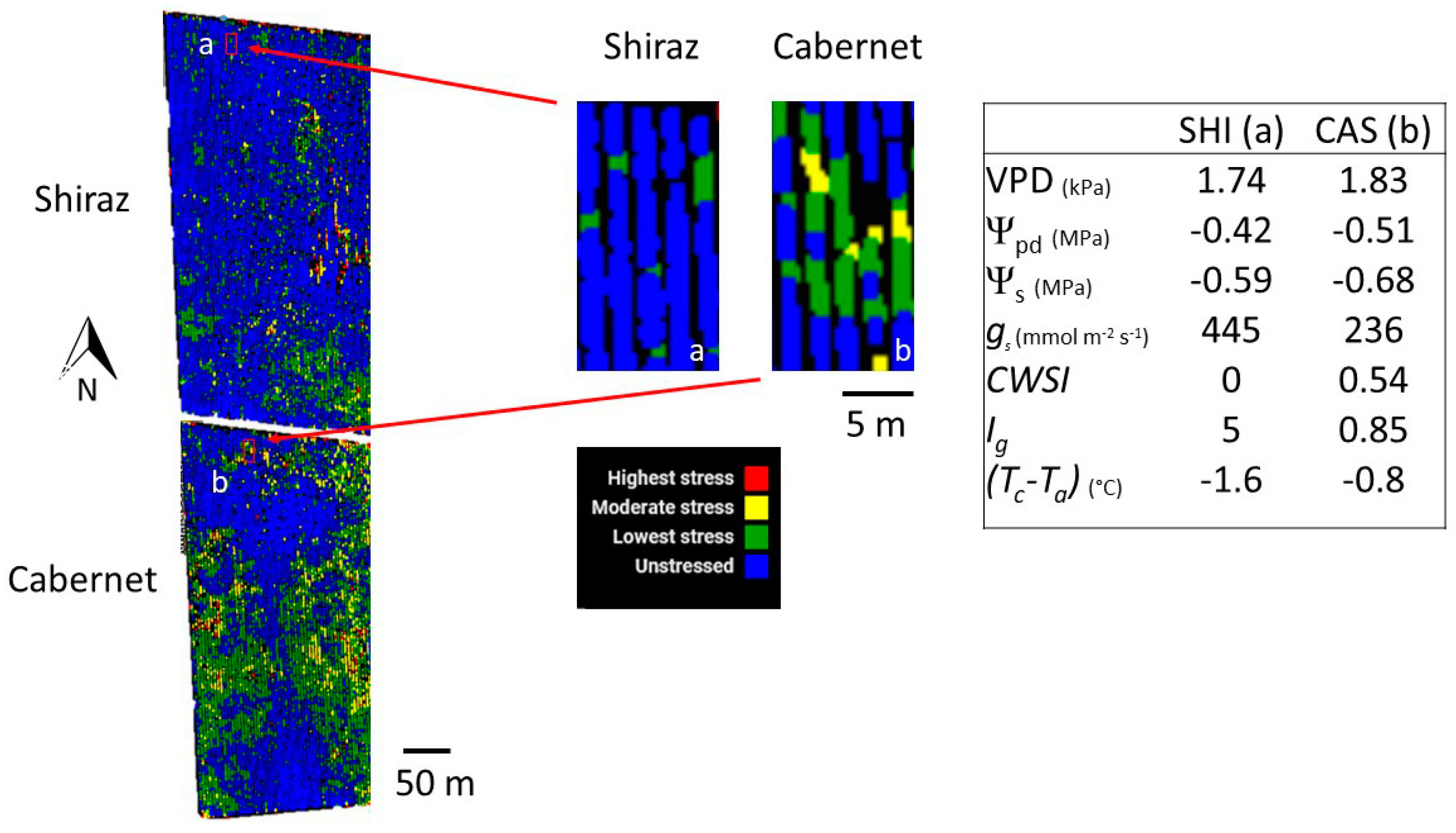
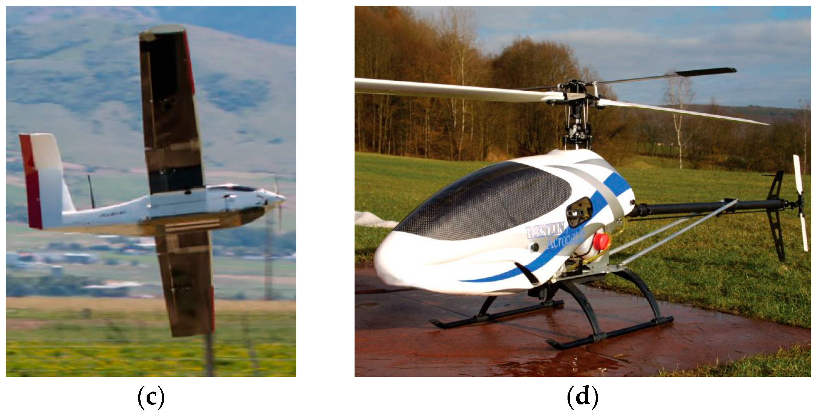
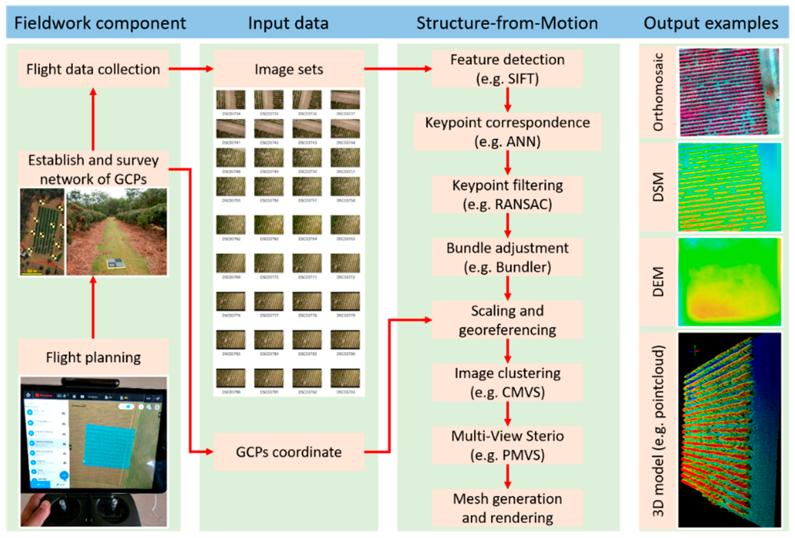
Table 1.
Some satellite systems that have been used to study the water status of horticultural crops.
Table 1.
Some satellite systems that have been used to study the water status of horticultural crops.
| Satellites | Band Numbers: Band Designation | Spatial Resolution (m) | Revisit Cycle |
|---|---|---|---|
| Landsat 7 | 8: V 3, NIR 1, SWIR 2, TIR 1, Pan 1 | 15–60 | 16 days |
| Landsat 8 | 11: C 1, V 3, NIR 1, SWIR 2, Pan 1, Ci 1, TIR 2 | 15–100 | 16 days |
| Sentinel-2 | 13: C 1, V 3, RE 3, NIR 2, WV 1, Ci 1, SWIR 2 | 10–60 | 5 days |
| Spot-6 and-7 | 5: Pan 1, V 3, NIR 1 | 1.5 | 1 day |
| RapidEye | 5: V 3, NIR 1, RE 1 | 5 | 5.5 days |
| GeoEye-1 | 5: Pan 1, V 3, NIR 1 | 0.41–2 | 3 days |
Note: Superscript integers 1, 2, 3 represent the number of bands; V = visible, NIR = near infrared, SWIR = short-wave infrared, TIR = thermal infrared, Pan = panchromatic, C = coastal, Ci = cirrus, RE = red edge, WV = water vapour.
Table 2.
Commonly used vegetation and thermal indices to study the water status of horticultural crops.
Table 2.
Commonly used vegetation and thermal indices to study the water status of horticultural crops.
| Indicators | Sensor | Purpose | References |
|---|---|---|---|
| Tc, (Tc − Ta) | Thermal | Ψstem, gs, yield | [34,82,85,99,110] |
| Ig, I3 | Thermal | Ψstem, gs | [82,196] |
| CWSI | Thermal | Ψleaf, Ψstem, gs, Pn, yield | [18,31,33,85,90,97,99,100,182,194,197,198,199] |
| (Tc − Ta)/NDVI | Thermal + multispectral | Ψstem, gs | [82,200] |
| NDVI | Multispectral | Ψstem, gs, yield, LAI, vigour | [34,56,82,86,182,201] |
| GNDVI | Multispectral | Ψstem, gs, yield | [34,82] |
| RDVI | Multispectral | Ψstem, gs | [82,86,182] |
| PRI | Multispectral | Ψleaf, gs | [86,110,182] |
| Fluorescence | Hyperspectral | Ψleaf, gs | [110] |
| WBI | Hyperspectral | Ψleaf, gs | [139,202,203] |
| SIF | Hyperspectral | Water stress | [204,205,206] |
Note the acronyms: Tc = Canopy temperature, Ta = ambient temperature, Ig = conductance index, I3 = stomatal conductance index, CWSI = crop water stress index, NDVI = normalised difference vegetation index, GNDVI = green normalised difference vegetation index, RDVI = renormalized difference vegetation index, PRI = photochemical reflectance index, Fluorescence = chlorophyll fluorescence, WBI = water band index, SIF = solar-induced chlorophyll fluorescence, LAI = leaf area index.
© 2020 by the authors. Licensee MDPI, Basel, Switzerland. This article is an open access article distributed under the terms and conditions of the Creative Commons Attribution (CC BY) license (http://creativecommons.org/licenses/by/4.0/).
Share and Cite
MDPI and ACS Style
Gautam, D.; Pagay, V. A Review of Current and Potential Applications of Remote Sensing to Study the Water Status of Horticultural Crops. Agronomy 2020, 10, 140. https://doi.org/10.3390/agronomy10010140
AMA Style
Gautam D, Pagay V. A Review of Current and Potential Applications of Remote Sensing to Study the Water Status of Horticultural Crops. Agronomy. 2020; 10(1):140. https://doi.org/10.3390/agronomy10010140
Chicago/Turabian StyleGautam, Deepak, and Vinay Pagay. 2020. "A Review of Current and Potential Applications of Remote Sensing to Study the Water Status of Horticultural Crops" Agronomy 10, no. 1: 140. https://doi.org/10.3390/agronomy10010140
Note that from the first issue of 2016, this journal uses article numbers instead of page numbers. See further details here.