Genome-Wide Association and Genomic Prediction for Fry Color in Potato


Teagasc, Crop Science Department, Oak Park, R93XE12 Carlow, Ireland
*
Author to whom correspondence should be addressed.
Agronomy 2020, 10(1), 90; https://doi.org/10.3390/agronomy10010090
Submission received: 2 December 2019
/
Revised: 13 December 2019
/
Accepted: 24 December 2019
/
Published: 9 January 2020
(This article belongs to the Special Issue Potato Genetics and Breeding in the Genomics Era)
Abstract
:Potatoes destined for crisping are normally stored above 8 degrees; below this glucose accumulates leading to very dark fry colors and potential acrylamide build up. Unfortunately, sprouting occurs above 4 degrees and impacts product quality, necessitating the use of sprout suppressant chemicals. Therefore, a goal of breeders is to develop potatoes with excellent fry color, which is maintained under storage below 8 degrees. Genomic or marker-assisted selection offers an opportunity to improve the efficiency of potato breeding and thereby assist breeders in achieving this goal. In this study, we have accumulated fry-color data on a large population of potato lines and combined this with genotypic data to carry out a GWAS and to evaluate accuracy of genomic prediction. We were able to identify a major QTL on chromosome 10 for fry color, and predict fry color with moderate accuracy using genome-wide markers. Furthermore, our results provide evidence that it is possible to identify a small subset of SNPs for processing characteristics that can give moderate predictive ability, albeit lower than that achieved with genome-wide markers.
1. Introduction
Conventional phenotypic selection is carried out by many potato breeders. In the breeding program at Teagasc a cycle of breeding is initiated each year with 200–300 pair-crosses that produce over 100,000 true seed. All target ideotypes are then selected from this base population over the next 12 years. In the early years negative selection is employed to reduce the number of seedlings from 100,000 down to approximately 2500 by year four. Marker-Assisted Selection (MAS) is then employed to identify entries with favourable alleles against some common potato pests and diseases. By year seven the number of entries being evaluated has dropped to approximately 50, and at this point multi-location field trials are carried out to record accurate phenotypes for a large suite of traits. A further seven years of multi-environment trialing and phenotyping typically yields one to three varieties from a cycle of selection. A downside of this selection scheme is that our ability to collect phenotype information for many important traits in the first years of the program is limited. Clonal individuals are represented by single tubers in the first field generation, rising to three plots (single location) in the third field generation. Selection based largely on visually assessable characteristics in a single location and year carries the risk of eliminating individuals with favourable characteristics due to chance poor performance. It could be argued that a simple solution is simply to carry forward greater numbers, but most breeding programs are constrained by logistical and financial limitations which partly determine selection intensity. Providing more information on non-visually assessable traits earlier in the program provides a better decision-making framework for breeders in the early stages of a program. Approaches to improve genetic gain in potato breeding using pedigree or genomic information have recently been discussed [1,2].
One approach using best linear unbiased prediction (BLUP) analysis with pedigree information to estimate breeding values has already been shown to lead to increased genetic gains, particularly for low heritability traits [2]. Genomic selection uses phenotyped and genotyped entries from a training set to predict phenotypes of new individuals based only on genomic information and has already been evaluated in various crop species [3,4,5,6]. A recent review concluded that genetic gain can be substantially improved by implementing genomic selection in potato breeding programs [1], and a recent study has also demonstrated empirically that genomic prediction for processing traits shows promise [7]. Genomic selection may be particularly beneficial when many traits can be selected for using the same genotyping data. An example would be developing potato varieties for the processing industry where a variety needs to have favourable performance for a large suite of traits, including fry color, yield, sugar stability under storage, percentage dry matter, tuber shape, flesh color, skin color, eye depth, tuber number, Potato Cyst Nematode (PCN) resistance, bruising, common scab, powdery scab, spraing resistance, blackleg resistance, blight resistance, and Potato Virus Y (PVY) resistance. A body of work has already been completed in an attempt to identify QTL or genes linked to processing characteristics [3,8,9,10,11,12,13,14,15].
A prerequisite for genomic selection is a genotyped and phenotyped training population for model development. The reduced cost of sequencing and the availability of genomic resources such as a reference genome [16] make it now feasible to characterize genetic variation on a genome-wide scale in potato populations. A greater challenge is the collection of accurate phenotypes for all target traits on the reference population. This is challenging due to time and cost of multi-year and multi-environmental trials on a sufficient number of lines to establish a training population. Resource constraints mean that the most efficient way to collect such data is to aggregate it from later stages of active breeding programs. However, there are generally much lower numbers of breeding lines under selection at these stages, meaning data must be aggregated over longer periods to enable sufficient population sizes. Other issues, such as unbalanced datasets and the fact that selection may have reduced allelic variation at this stage may also be problematic.
In this study, we have collected phenotypes and genotypes for multiple reference populations consisting of entries under evaluation in the Teagasc breeding program. These data were then used to build genomic prediction models that were evaluated on testing sets not used for training. Predictive abilities varied from low to moderate depending on the training and testing sets used. Interestingly, our results suggest that marker number can be greatly reduced with limited impact on predictive ability; that may permit deployment of inexpensive marker assays for prediction of potato processing characteristics.
2. Results
2.1. Genotyping and Phenotyping Potato Lines
We accumulated phenotypic data on lines over three years (2015–2017) from material undergoing evaluation in the third field generation of the Teagasc breeding program. Each line was only evaluated in a single year and location. At the 2015 harvest we processed tubers three weeks after harvest (referred to as ‘off-the-field’) and also stored tubers for extended periods at either C, or C with chlorpropham treatment. The correlations between data sets were high (Table 1) and in general we observed that entries which had very light fry color (as measured by the HunterLab L value) when fried ‘off-the-field’ tended to have very light fry colors when fried after long-term storage.
In subsequent years we focused our phenotyping efforts on material ‘off-the-field’ (OTF) and after long-term storage (LTS) at C for 230 days and from this point on we will only discuss results related to these time-points. It is clear from the results that the median HunterLab L values for fry color in the training population were greatest in the data set fried ‘off-the-field’, and there was a distinct decrease in median HunterLab L values for tubers stored at C (Figure 1). The mean HunterLab L values for the populations fried ‘off-the-field’ was 13 to 26% higher than tubers stored at C for ca. seven months.
Additionally, phenotypes were available for lines that had been evaluated for fry-color OTF in multiple locations and over multiple year (referred to as test panel). All lines were genotyped using a genotyping-by-sequencing approach after genome complexity reduction with the restriction enzyme ApeKI. The sequencing depth required to distinguish between the three heterozygous states in autotetraploid potato has been estimated at 60 [17]. As we did not have sufficient sequencing depth at each locus we treated the samples as diploids and determined genotypes according to rules developed in autotetraploid alfalfa [18]. A SNP database of 46,406 SNPs was developed using genotype data from all lines, and was used for developing genomic prediction models for fry color, and also for QTL identification with a GWAS. The SNP database had SNPs covering all potato chromosomes, and the number of SNPs ranged from 2707 on chromosome 10 to 5424 on chromosome 1. SNPs clustered towards the telomeres, which corresponds to regions of much higher gene density in potato [16]. It also confirms that Genotyping-By-Sequencing (GBS) with ApeKI digestion (methylation sensitive) in potato largely avoids the heterochromatin located in the pericentromeric regions. On average the SNP rate across the genome is one SNP every 17,469 bases; however, GBS is only interrogating regions around a portion of the ApeKI restriction sites. SNPs were well distributed across all genomic regions (downstream: 27.99%, exon: 22.30%, intergenic: 11.00%, intron: 11.42%, upstream: 20.18%, utr: 6.40%, splice sites: 0.71%), with 13,407 genes tagged with at least one SNP. Lines with more than 10,000 missing genotypes (22%) were removed and remaining lines with matching phenotype and genotype data were used for GWAS and genomic prediction (Table 2).
2.2. Genome-Wide Association Analysis
A GWAS was performed within each year separately to identify significant QTL for fry color ‘off-the-field’ and after long-term storage at C. We did not identify any SNPs significantly associated with fry color after long-term storage at C in any of the three populations. However, we did identify QTL significantly associated with fry color ‘off-the-field’ in the 2017 population; the largest population available for analysis (Table 3, Figure 2). We identified significantly associated SNPs on chr04 and chr10, with the strongest signal on chr10. The SNPs on chr04 (chr04:67971220 and chr04:68008112) are proximal to a tuber-specific and sucrose-responsive element binding factor (PGSC0003DMG400003316, chr04:67630128–67632587).
The greatest number of SNPs were located on chr10 within the region from 49 Mb to 58 Mb, and several genes associated with sucrose cleavage, synthesis, metabolism and starch storage are located within the 50 to 60 Mb region of chr10 [16]. These include three invertase inhibitors, a sucrose-phosphatase, a cell-wall invertase, a fructose-1,6-biphosphatase, and two patatin genes.
2.3. Using Genome-Wide Variants to Predict Fry Color
We developed genomic prediction models with data from each of the three years, and used these to predict fry color ‘off-the-field’ and fry color after long-term storage at C in the remaining years. We also used the three models to predict fry color ‘off-the-field’ in a test panel made up of advanced breeding lines from multiple years at later stages of the Teagasc breeding program. The mean predictive ability ranged between 0.11 and 0.77 for fry color ‘off-the-field’, and between 0.24 and 0.66 for fry color after long-term storage at C (Table 4).
Our ability to predict ‘off-the-field’ fry color was greater than our ability to predict fry color after long-term storage at C, likely reflecting the additional complexity of the trait and in keeping with our ability to detect QTL for the former but not the latter. There was little difference in predictive ability across the different models evaluated, with the exception of the models developed using Random Forest, which resulted in lower predictive ability in all cases.
The predictive ability dropped when 2016 data was used as either training or test panel. It can be seen from the Genomic Relationship Matrix (GRM) (Figure 3) that the lines from 2016 set have a low relationship to the other populations, which likely explains the poorer predictive ability when 2016 was used as either a training or testing set. Conversely, we can see many high intensity genomic relationship values between lines in 2015 and 2017, which likely explains the greater predictive ability when these are used as training and testing sets.
2.4. Using Selected Variants to Predict Fry Color
We also developed predictive models using a subset of SNPs identified in the GWAS. Using the significant GWAS SNPs identified in the 2017 lines (31 SNPs), we were able to predict fry color ‘off-the-field’ in the 2015 population with a predictive ability of 0.45 and no bias.
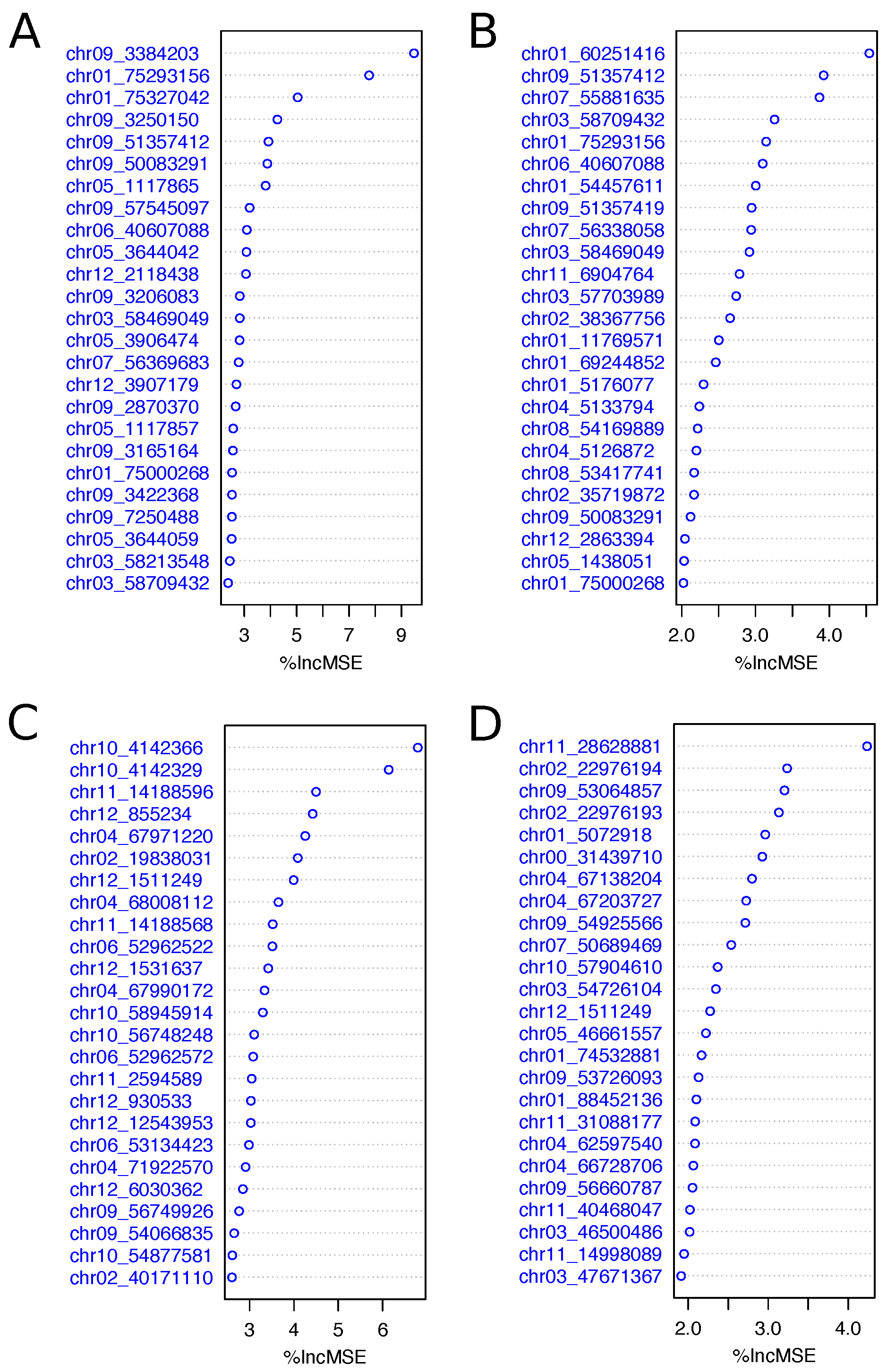
In addition to using the GWAS to select subsets of SNPs for prediction, we performed variable selection using the variable importance measures from Random Forest. This was done with the 2015 and 2017 data sets and for both fry color ‘off-the-field’ and after long-term storage at C. In all cases the top 25 variables were widely spread across chromosomes (Figure 4), and the two SNPs identified on chr04 with the GWAS in the 2017 data set were in the top 25 ranked SNPs identified using variable importance measures.
These SNPs were located at 67.97 and 68.00 Mb and are proximal to a tuber-specific and sucrose-responsive element binding factor (PGSC0003DMG400003316, chr04:67630128), and an Alpha-amylase (PGSC0003DMG400007974, chr04:68255931) involved in starch degradation. The SNP on chr01 at 75.29 Mb that ranked high in importance in the 2015 data set is near three sugar transporters at 76.16–76.23 Mb; furthermore markers associated with fry color have been found on chr01 at 43.8 cM [8] and QTL have been identified in linkage mapping studies [9]. A number of SNPs in the top 25 in both data sets and for both traits were located on chr09 and markers associated with fry color have been identified in association panels on chr09 [8]. One SNP at 51.35 Mb identified as the second most important variable for fry color after long-term storage at C in 2015 data set was proximal to a gene involved in sugar transport (Sugar transporter, PGSC0003DMG400003848, chr09:51364561).
We used the variable importance measures to select increasing numbers of ranked SNPs to develop genomic selection models for prediction in the data set that was left out of both variable selection and model training. The predictive ability was higher with selected SNPs compared to a random SNPs at lower SNP numbers; however, the difference disappeared as we increased SNP number (Table 5).
3. Discussion
In this study, we present the results of a simple empirical evaluation of predicting fry color with DNA-based markers. Markers were generated using a genotyping-by-sequencing approach following genome complexity reduction with the restriction enzyme ApeKI. Predictive abilities were assessed as a function of statistical algorithm and marker density. We also present the results of a GWAS to identify QTL for fry color and low-temperature sweetening.
We did not observe any great difference between statistical algorithms in terms of predictive ability, which is in agreement with other studies [3,7,19]; with the exception that models developed with Random Forest had lower predictive ability. Predictive abilities were promising for both ‘off-the-field’ fry color and fry color after long-term storage at low-temperature. This is in general agreement with a recent study on genomic prediction of chipping quality in potato [7]. Our predictive ability was high (0.77) for ‘off-the-field’ fry color when training with the 2017 data set and predicting in 2015 data set. Similarly, when training with the 2015 data set and predicting in the 2017 data set, the predictive ability was 0.75. The predictive ability varied across training and test population combinations with the lowest predictive abilities observed when 2016 was used as either a training or testing set. This reflects the lower relationship between lines in 2016 and other data sets used. The lower levels of relatedness of the 2016 material was most likely due to the presence of entries from a parallel experimental program for pyramiding and multiplexing disease resistance loci in that year. This resulted in a different parental profile and lower rate of selection in this material. This is similar to previous studies in plants [20,21] and predictions across breeds in animals [22,23], and emphasises the importance of a good relationship between training set and selection candidates.
Our GWAS failed to identify QTL for resistance to low-temperature sweetening but did identify QTL for fry color ‘off-the-field’ in the 2017 data set. Two SNPs on chro04 at 67.97 and 68.00 Mb were associated with fry color. In particular the SNP at 67.97 Mb is proximal to a tuber-specific and sucrose-responsive element binding factor. These two SNPs were also identified with the variable importance measures in the 2017 data set. Previous studies have identified QTL for fry color in two association panels on chromosome four [8]. Our strongest QTL signal was on chr10 where a large cluster of associated SNPs was identified between 49 and 59 Mb, peaking at 55.28 Mb. Other genome-wide association studies looking at fry color have been carried out. A QTL for fry color has previously been detected at 57.6 Mb in a panel of varieties characterized by several Dutch breeding companies [8]. Another GWAS in a diversity panel did not identify QTL for processing quality [24] although the authors concluded that more lines and higher marker density were required. A recent study [7] also identified a cluster of SNPs associated with fry color on chromosome 10 in the region between 50 and 60 Mb, and our study now reproduces those findings in a different population; indicating that this may be an important region for fry color in potato. In future, genotyping approaches that enable distinction among the three heterozygous states, and support multi-allelic haplotype analysis may increase our power to detect marker-trait associations.
We selected all markers significantly associated with fry color in 2017 data set (31 SNPs) and used these to develop genomic selection models to predict fry color in 2015 data set, which resulted in a predictive ability (0.45), substantially lower than predictive ability with entire marker set. The majority of markers in this subset are within the 10 Mb region on chr10. We also identified and ranked variables using variable importance measures and selected increasing number for development of prediction models. In this case the marker subset is spread out across chromosomes. While predictive ability was lower than using entire marker set, it was higher than randomly selected markers at lower marker number. As we increase the marker number the difference between markers selected via variable importance measures and random selection reduced. Using the top 10 ranked SNPs our predictive ability for both traits ranged between 0.50 and 0.59 depending on which year was used as a training set. The ability to generate predictions with smaller sets of molecular markers is essential if we are to implement DNA-based selection strategies in classical potato phenotypic selection schemes.
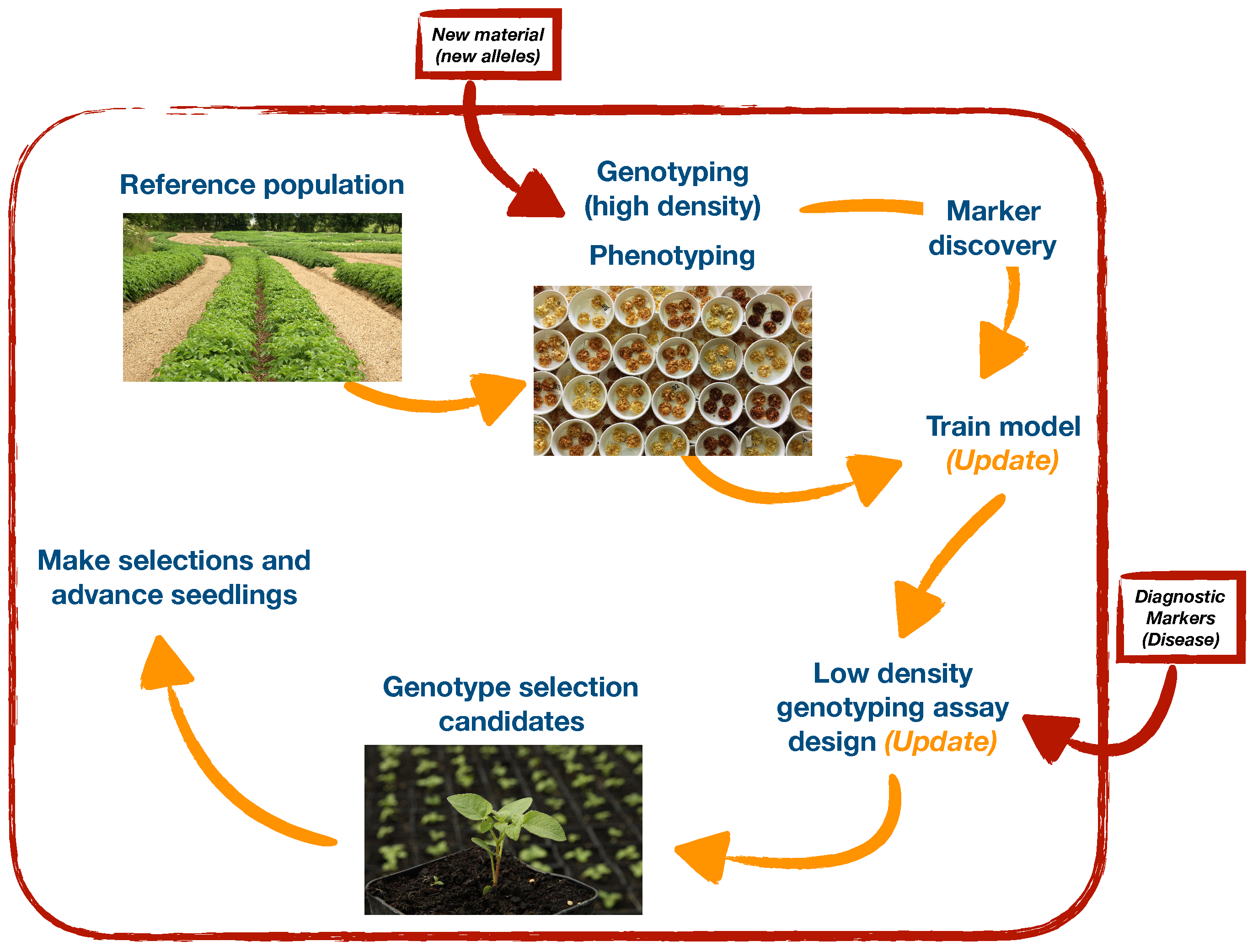
Various strategies to improve breeding in potato using pedigree [2] and/or marker-assisted selection strategies [1] have been proposed. In some cases these require significant alterations to breeding schemes, including the classical phenotypic selection scheme outlined. One of the downsides of these schemes is that our ability to phenotype and make accurate selections in early years is very low. There is an opportunity to practice DNA-based selection in these early years, provided low cost DNA evaluations can be carried out. Within our breeding program, marker-assisted selection using low cost diagnostic markers for disease resistance is already carried out on 1000’s of entries in single plot trials. Using genome-wide markers for selection in early stages of these schemes when numbers are large is currently not feasible; however, if we can identify smaller sets of markers that together have good predictive ability then there are opportunities to develop inexpensive marker systems [25] and practice marker-assisted selection for both simple (e.g., disease resistance) and more complex (e.g., processing) traits at high selection intensities. In particular, we envisage being able to develop a genotyping platform based on amplicon sequencing that is (i) inexpensive, (ii) multi-allelic, and (iii) adaptable (markers can easily be added or removed from the assay). An example of such an approach is outlined (Figure 5), which has the advantage of being flexible to enable inclusion of new loci and/or estimating the effects of new alleles as new material is introduced to the initial crossing schemes.
4. Conclusions
Experimental results presented in this manuscript provide further support for the implementation of genomic prediction in potato breeding, and further evidence for a major QTL on chromosome 10 for fry color. Furthermore, our results provide evidence that it is possible to identify informative SNPs for processing characteristics, and that these SNPs have predictive abilities approaching those of genome-wide marker sets.
5. Materials and Methods
5.1. Phenotyping Training and Test Panels
The training populations consisted of lines collected from the breeding program over a period of three years (2015–2017). Lines were evaluated in 20-tuber plots and each line was phenotyped in a single year. In 2015 the tubers were harvested on the 7th October 2015 and collected for storage and subsequent fry analysis. Tubers from each plot were divided into six batches of ten tubers for drying and storage at either C or C (with chlorpropham treatment for sprout suppression), and removed for phenotyping at various time-points (Table 1). Four tubers (from the same plot) were selected from each entry at each time point and fried to evaluate crisp color. Tubers were sliced with a Hobert slicer to generate crisps with a thickness of 1.25 mm, and were deep fried for three minutes at C. Crisp color was then measured using a HunterLab Labscan XE Spectrophotometer (400–700 nm) in an upward configuration through a transparent petri-dish. Hunter L values were recorded, which indicates the level of lightness or darkness of crisps. Sample preparation and presentation were kept consistent across years to avoid variation due to sample preparation/presentation. The arithmetic mean of the four samples from each entry was calculated and used in subsequent analysis. In subsequent years (2016–2017) we focused phenotyping on samples collected off-the-field and those stored at C for ca. seven months. Again, the arithmetic mean of four tubers from each entry was calculated and used in subsequent analysis (https://doi.org/10.6084/m9.figshare.11298941).
The testing panel consisted of 56 lines with data on fry color ‘off-the-field’, which was collected as part of the breeding program over a six year period (2012–2017) with up to five locations per year and three replicate plots per location. Fry color was evaluated using a HunterLab Labscan XE Spectrophotometer, and not all 67 lines were evaluated together in a common field site, making it a highly unbalanced data set. BLUPs for fry color of each line were calculated using line as a random effect and year, location and the interaction as fixed effects.
5.2. Genotyping Training and Testing Panels
Leaf material was harvested from each entry and freeze dried for 48 h prior to tissue disruption on a bead mill and DNA isolation. DNA was isolated using a modified version of the CTAB protocol [26], and pellets were dissolved in 100 L of TE 0.1 mM EDTA and treated with RNAse A for removal of RNA contamination. DNA samples were transferred to 96-well plates, quantified using a PicoGreen Quant-It ds-DNA assay, and all samples diluted to 20 ng/L. The Genotyping-By-Sequencing (GBS) protocol followed that of [27]. Briefly, DNA from each sample was digested with the restriction enzyme ApeKI that has a 5 bp recognition site. Digested DNA was ligated to adaptors containing one of 96 unique DNA barcodes and up to 96 samples were then pooled to generate a single library. Each library was amplified via PCR, quantified, and evaluated on a BioAnalyser prior to sequencing. Each library was sequenced on 2–3 lanes of an Illumina HiSeq 2500 to generate single-end (SE) reads of 100 bp.
Sequence data from the same library was concatenated and adaptor contamination was removed with Scythe [28] with a prior contamination rate set to 0.40. Sickle [29] was used to trim reads when the average quality score in a sliding window (of 20 bp) fell below a phred score of 20, and reads shorter than 40 bp were discarded. The reads were demultiplexed using Sabre [30] allowing a single mismatch, data output per sample was determined, and reads from each sample were aligned to the Solanum tuberosum reference genome [16] using BWA aln with default parameters [31]. The Genome Analysis Tool Kit (GATK) [32] was used to identify putative SNPs in the population, and only SNPs with a read map score of 30 were retained for further analysis. We used an approach developed in alfalfa for calling genotypes from GBS data in autotetraploids [18], where distinguishing between three heterozygous states is difficult with low read depth. Briefly, no attempt was made to distinguish between the three different heterozygous states present in an autotetraploid (ABBB, AABB, AAAB), a minimum of 11 reads were required to confirm a homozygote, and a minimum of two reads per allele and a minimum allele frequency for alternative allele of 0.10 were required to call a heterozygote. The minor allele frequency (MAF) was calculated based on these genotype calls and SNPs with a MAF ≥2.5% and with ≤15% missing genotype data were retained for further analysis. Sequence data have been submitted to NCBI under BioProject PRJNA566151.
5.3. GWAS to Identify QTL Associated with Fry Color
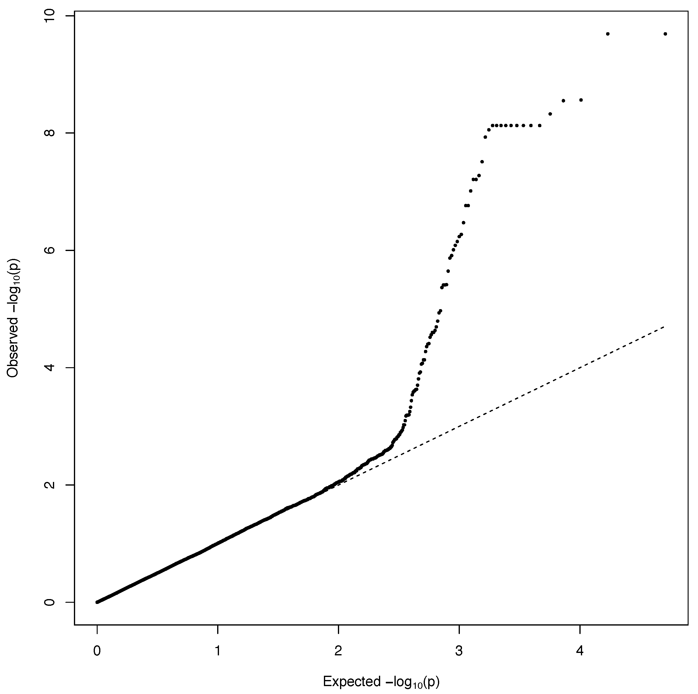
A GWAS was carried out separately on data from each year with the R package GWASpoly [24]. All heterozygous genotypes were treated as having the same effect (diploidized additive), and kinship was calculated using the realized relationship matrix (see QQ-Plot; Figure 6). The genome-wide false discovery rate was controlled using Bonferroni method (level = 0.05).
5.4. Genomic Prediction of Fry Color
We used four statistical algorithms for genomic prediction, ridge regression best linear unbiased predictor (rrBLUP) [33], Bayes A [34], Bayesian Lasso [35] and Random Forest [36]. rrBLUP was used to estimate marker effects in the R package rrBLUP [33], the two Bayesian approaches were implemented in the R package BGLR [37] with the following parameters: number of iterations = 5000, burn-in = 500 and thinning = 5. Random forest was implemented with the R package Random Forest (setting the number of variables at each split to 1/3 of the total variables, and using a terminal node size of five and minimum of 500 trees per forest). Predictive ability was calculated as the Pearson correlation coefficient between observed and predicted values.
Genomic prediction models were developed for each year and evaluated in other years. Predictive models developed for fry color ‘off-the-field’ in each year (2015–2017) were also evaluated in a test panel consisting of 56 lines.
We also selected markers from the GWAS to use in genomic prediction. The GWAS was carried out in the training population as described above and selected markers were used to build prediction models with the training population. These prediction models were then used for prediction in the testing population. Variable importance measures were carried out in Random Forest using the mean decrease in accuracy as the importance measure.
Author Contributions
D.M., D.G. and S.B. conceived and designed the study. C.K. managed the field and storage trials. F.M. (Francesca Mesiti) and F.M. (Fergus Meade) isolated DNA, and optimized and carried out the genotyping of training and testing populations. F.M. (Francesca Mesiti), S.B. and F.M. (Fergus Meade) carried out the phenotyping. S.B. performed data analysis, and drafted the initial manuscript. All authors contributed to interpretation of data and preparation of final manuscript. All authors have read and agreed to the published version of the manuscript.
Funding
This project has received funding from the European Union’s Horizon 2020 research and innovation program under the Marie Sklodowska-Curie grant agreement number 658031. The project is also supported by the Irish Department of Agriculture, Food and the Marine (DAFM) through the Virtual Irish Centre for Crop Improvement (VICCI) (Project no. 14/S/819).
Acknowledgments
We gratefully acknowledge the support of IPM Potato Group Limited to the potato breeding program.
Conflicts of Interest
The authors declare no conflict of interest.
References
- Slater, A.T.; Cogan, N.O.; Forster, J.W.; Hayes, B.J.; Daetwyler, H.D. Improving genetic gain with genomic selection in autotetraploid potato. J. Abbr. 2016, 9. [Google Scholar] [CrossRef] [PubMed] [Green Version]
- Slater, A.T.; Wilson, G.M.; Cogan, N.O.; Forster, J.W.; Hayes, B.J. Improving the analysis of low heritability complex traits for enhanced genetic gain in potato. Theor. Appl. Genet. 2014, 127, 809–820. [Google Scholar] [CrossRef] [PubMed]
- Annicchiarico, P.; Nazzicari, N.; Li, X.; Wei, Y.; Pecetti, L.; Brummer, E.C. Accuracy of genomic selection for alfalfa biomass yield in different reference populations. BMC Genom. 2015, 16, 1020. [Google Scholar] [CrossRef] [PubMed] [Green Version]
- F‘e, D.; Pedersen, M.G.; Jensen, C.S.; Jensen, J. Genomic prediction of seedling root length in maize (Zea mays L.). Plant J. 2015, 83, 903–912. [Google Scholar]
- Pace, J.; Yu, X.; Lubberstedt, T. Genetic and environmental variation in a commercial breeding program of perennial ryegrass. Crop Sci. 2015, 55, 631–640. [Google Scholar]
- Ramstein, G.; Evans, J.; Kaeppler, S.; Mitchell, R.; Vogel, K.; Buell, C.; Casler, M.T. Accuracy of genomic prediction in switchgrass (Panicum virgatum L.) improved by accounting for linkage disequilibrium. G3 2016, 6, 1049–1062. [Google Scholar] [CrossRef] [Green Version]
- Sverrisdottie, E.; Byrne, S.; Sundmark, E.H.R.; Johnsen, H.O.; Kirk, H.G.; Asp, T.; Janss, L.; Nielsen, K.L. Genomic prediction of starch content and chipping quality in tetraploid potato using genotyping-by-sequencing. Theor. Appl. Genet. 2017, 130, 2091–2108. [Google Scholar] [CrossRef]
- Björn, B.; Keizer, P.L.; Paulo, M.J.; Visser, R.G.; van Eeuwijk, F.A.; van Eck, H.J. Identification of agronomically important QTL in tetraploid potato cultivars using a marker-trait association analysis. Theor. Appl. Genet. 2014, 127, 731–748. [Google Scholar]
- Bradshaw, J.E.; Hackett, C.A.; Pande, B.; Waugh, R.; Bryan, G.J. QTL mapping of yield, agronomic and quality traits in tetraploid potato (Solanum tuberosum subsp. tuberosum). Theor. Appl. Genet. 2008, 116, 193–211. [Google Scholar] [CrossRef]
- Björn, B.; Paulo, M.J.; Mank, R.A.; Van Eck, H.J.; Van Eeuwijk, F.A. Association mapping of quality traits in potato (Solanum tuberosum L.). Euphytica 2008, 161, 47–60. [Google Scholar]
- Menéndez, C.M.; Ritter, E.; Schäfer-Pregl, R.; Walkemeier, B.; Kalde, A.; Salamini, F.; Gebhardt, C. Cold sweetening in diploid potato: Mapping quantitative trait loci and candidate genes. Genetics 2002, 162, 1423–1434. [Google Scholar] [PubMed]
- Li, L.; Tacke, E.; Hofferbert, H.R.; Lübeck, J.; Strahwald, J.; Draffehn, A.M.; Walkemeier, B.; Gebhardt, C. Validation of candidate gene markers for marker-assisted selection of potato cultivars with improved tuber quality. Theor. Appl. Genet. 2013, 126, 1039–1052. [Google Scholar] [CrossRef] [Green Version]
- Fischer, M.; Schreiber, L.; Colby, T.; Kuckenberg, M.; Tacke, E.; Hofferbert, H.R.; Schmidt, J.; Gebhardt, C. Novel candidate genes influencing natural variation in potato tuber cold sweetening identified by comparative proteomics and association mapping. BMC Plant Biol. 2013, 13, 113. [Google Scholar] [CrossRef] [PubMed] [Green Version]
- Schreiber, L.; Nader-Nieto, A.C.; Schönhals, E.M.; Walkemeier, B.; Gebhardt, C. SNPs in genes functional in starch-sugar interconversion associate with natural variation of tuber starch and sugar content of potato (Solanum tuberosum L.). G3 Genes Genom. Genet. 2014, 4, 1797–1811. [Google Scholar] [CrossRef] [PubMed] [Green Version]
- Li, L.; Paulo, M.J.; Strahwald, J.; Lübeck, J.; Hofferbert, H.R.; Tacke, E.; Junghans, H.; Wunder, J.; Draffehn, A.; van Eeuwijk, F.; et al. Natural DNA variation at candidate loci is associated with potato chip color, tuber starch content, yield and starch yield. Theor. Appl. Genet. 2008, 116, 1167–1181. [Google Scholar] [CrossRef] [Green Version]
- Potato Genome Sequencing Consortium. Genome sequence and analysis of the tuber crop potato. Nature 2011, 475, 189–195. [Google Scholar] [CrossRef]
- Uitdewilligen, J.G.; Wolters, A.M.A.; Bjorn, B.; Borm, T.J.; Visser, R.G.; van Eck, H.J. A next-generation sequencing method for genotyping-by-sequencing of highly heterozygous autotetraploid potato. PLoS ONE 2013, 8, e62355. [Google Scholar] [CrossRef] [Green Version]
- Li, X.; Wei, Y.; Acharya, A.; Jiang, Q.; Kang, J.; Brummer, E.C. A saturated genetic linkage map of autotetraploid alfalfa (Medicago sativa L.) developed using genotyping-by-sequencing is highly syntenous with the Medicago truncatula genome. G3 Genes Genom. Genet. 2014, 4, 1971–1979. [Google Scholar]
- Tan, B.; Grattapaglia, D.; Martins, G.S.; Ferreira, K.Z.; Sundberg, B.; Ingvarsson, P.K. Evaluating the accuracy of genomic prediction of growth and wood traits in two eucalyptus species and their f 1 hybrids. BMC Plant Biol. 2017, 17, 110. [Google Scholar] [CrossRef] [Green Version]
- Wang, Y.; Mette, M.F.; Miedaner, T.; Gottwald, M.; Wilde, P.; Reif, J.C.; Zhao, Y. The accuracy of prediction of genomic selection in elite hybrid rye populations surpasses the accuracy of marker-assisted selection and is equally augmented by multiple field evaluation locations and test years. BMC Genom. 2014, 15, 556. [Google Scholar] [CrossRef] [Green Version]
- Nielsen, N.H.; Jahoor, A.; Jensen, J.D.; Orabi, J.; Cericola, F.; Edriss, V.; Jensen, J. Genomic prediction of seed quality traits using advanced barley breeding lines. PLoS ONE 2016, 11, 0164494. [Google Scholar] [CrossRef] [PubMed] [Green Version]
- Habier, D.; Tetens, J.; Seefried, F.-R.; Lichtner, P.; Thaller, G. The impact of genetic relationship information on genomic breeding values in german holstein cattle. Genet. Sel. Evol. 2010, 42, 5. [Google Scholar] [CrossRef] [PubMed] [Green Version]
- Riggio, V.; Abdel-Aziz, M.; Matika, O.; Moreno, C.; Carta, A.; Bishop, S. Accuracy of genomic prediction within and across populations for nematode resistance and body weight traits in sheep. Animal 2014, 8, 520–528. [Google Scholar] [CrossRef] [Green Version]
- Rosyara, U.R.; De Jong, W.S.; Douches, D.S.; Endelman, J.B. Software for genome-wide association studies in autopolyploids and its application to potato. Plant Genome 2016, 9. [Google Scholar] [CrossRef] [Green Version]
- Campbell, N.R.; Harmon, S.A.; Narum, S.R. Genotyping-in-thousands by sequencing (gt-seq): A cost effective snp genotyping method based on custom amplicon sequencing. Mol. Ecol. Resour. 2015, 15, 855–867. [Google Scholar] [CrossRef] [PubMed]
- Doyle, J.J.; Doyle, J.L. A rapid DNA isolation procedure for small quantities of fresh leaf tissue. Phytochem. Bull. 1987, 19, 11–15. [Google Scholar]
- Elshire, R.J.; Glaubitz, J.C.; Sun, Q.; Poland, J.A.; Kawamoto, K.; Buckler, E.S.; Mitchell, S.E. A robust, simple genotyping-by-sequencing (gbs) approach for high diversity species. PLoS ONE 2011, 6, 19379. [Google Scholar] [CrossRef] [Green Version]
- Buffalo, V. Scythe—A Bayesian Adapter Trimmer Version 0.994 Beta. Available online: https://github.com/vsbuffalo/scythe (accessed on 7 November 2015).
- Joshi, F. Sickle—A Windowed Adaptive Trimming Tool for Fastq Files Using Quality. 2011. Available online: https://github.com/ucdavis-bioinformatics/sickle (accessed on 7 November 2015).
- Joshi, F. Sabre—A Barcode Demultiplexing and Trimming Tool for Fastq Files. 2011. Available online: https://github.com/najoshi/sabre (accessed on 7 November 2015).
- Li, H.; Durbin, R. Fast and accurate short read alignment with burrows–wheeler transform. Bioinformatics 2009, 25, 1754–1760. [Google Scholar] [CrossRef] [Green Version]
- De Pristo, M.A.; Banks, E.; Poplin, R.; Garimella, K.V.; Maguire, J.R.; Hartl, C.; Philippakis, A.A.; Del Angel, G.; Rivas, M.A.; Hanna, M. A framework for variation discovery and genotyping using next-generation dna sequencing data. Nat Genet. 2011, 43, 491–498. [Google Scholar] [CrossRef]
- Endelman, J.B. Ridge regression and other kernels for genomic selection with R package rrBLUP. Plant Genome 2011, 4, 250–255. [Google Scholar] [CrossRef] [Green Version]
- Meuwissen, T.; Hayes, B.; Goddard, M. Prediction of total genetic value using genome-wide dense marker maps. Genetics 2001, 157, 1819–1829. [Google Scholar] [PubMed]
- Park, T.; Casella, G. The bayesian lasso. J. Am. Stat. Assoc. 2008, 103, 681–686. [Google Scholar] [CrossRef]
- Liaw, A.; Wiener, M. Classification and regression by randomForest. R News 2002, 2, 18–22. [Google Scholar]
- De los Campos, G.; Pérez-Rodríguez, P. Bayesian Generalized Linear Regression. Available online: https://rdrr.io/cran/BGLR/ (accessed on 12 December 2019).
Figure 1.
Boxplot of fry color of three populations through storage. Fry color measured as HunterLab L-values when fried ‘off-the-field’ (OTF) and after long-term storage at C for ca. seven months post-harvest.
Figure 1.
Boxplot of fry color of three populations through storage. Fry color measured as HunterLab L-values when fried ‘off-the-field’ (OTF) and after long-term storage at C for ca. seven months post-harvest.

Figure 2.
Results of a GWAS for ‘off-the-field’ fry color (OTF) in 2017 population—genome-wide (left) and zoomed in on chromosome 10 (right). Red line shows the QTL significance threshold (Bonferronni correction, level = 0.05).
Figure 2.
Results of a GWAS for ‘off-the-field’ fry color (OTF) in 2017 population—genome-wide (left) and zoomed in on chromosome 10 (right). Red line shows the QTL significance threshold (Bonferronni correction, level = 0.05).

Figure 3.
Heatmap of the Genomic Relationship Matrix (GRM). Lines belonging to the test panel are shown in red, lines from 2015 are shown in green, lines from 2016 are shown in blue, and lines from 2017 are shown in grey.
Figure 3.
Heatmap of the Genomic Relationship Matrix (GRM). Lines belonging to the test panel are shown in red, lines from 2015 are shown in green, lines from 2016 are shown in blue, and lines from 2017 are shown in grey.

Figure 4.
Variable (SNPs) importance measures calculated for fry color ‘off-the-field’ in 2015 (A) and 2017 (C), and after long-term storage at C in 2015 (B) and 2017 (D). The x-axis indicates the increase of the Mean Squared Error (MSE) when the SNP is randomly permuted. The top 25 variables are shown.

Figure 5.
Pathway to implementation of marker-assisted selection in potato breeding. An initial reference population representing the breeding material is both genotyped and phenotyped for target traits. These data can be used to identify markers linked to traits and develop prediction models. Markers linked to QTL for complex traits and markers diagnostic for disease resistance can be used in development of an inexpensive genotyping assay for deployment on selection candidates.

Figure 6.
QQ-Plot for ‘off-the-field’ fry color in 2017 population.


Table 1.
Correlation of fry color between storage treatments. Pearson correlation coefficients comparing fry color of the tubers harvested in 2015 (n = 274) stored under different conditions and lengths of time (shown as days post-harvest).
Table 1.
Correlation of fry color between storage treatments. Pearson correlation coefficients comparing fry color of the tubers harvested in 2015 (n = 274) stored under different conditions and lengths of time (shown as days post-harvest).
| OTF | C + 104d | C + 237d | C + 111d | C + 183d | C + 230d | |
|---|---|---|---|---|---|---|
| OTF | 1 | |||||
| C + 104d | 0.92 | 1 | ||||
| C + 237d | 0.84 | 0.88 | 1 | |||
| C + 111d | 0.84 | 0.91 | 0.86 | 1 | ||
| C + 183d | 0.78 | 0.87 | 0.83 | 0.91 | 1 | |
| C + 230d | 0.77 | 0.86 | 0.83 | 0.90 | 0.91 | 1 |
Table 2.
Number of lines with sufficient genotype and phenotype data for further analysis. The three populations (2015–2017) from the third field evaluation year were used for GWAS and development of genomic prediction models. A collection of lines from highly unbalanced multi-location and multi-year trials (test panel) was used to further evaluate the prediction models developed with the 2015–2017 data.
| Population | OTF | LTS |
|---|---|---|
| 2015 | 192 | 192 |
| 2016 | 45 | 88 |
| 2017 | 219 | 219 |
| test panel | 56 | - |
Table 3.
Genome-wide association study of fry color off-the-field in 2017 population. SNP significantly associated with fry-color (Bonferronni correction, level = 0.05); SNPs are sorted by chromosome and position.
Table 3.
Genome-wide association study of fry color off-the-field in 2017 population. SNP significantly associated with fry-color (Bonferronni correction, level = 0.05); SNPs are sorted by chromosome and position.
| Chrom | bp | −log10(p) |
|---|---|---|
| chr04 | 67971220 | 6.23 |
| chr04 | 68008112 | 5.91 |
| chr10 | 49770199 | 6.15 |
| chr10 | 53208176 | 5.87 |
| chr10 | 54783863 | 8.33 |
| chr10 | 54800561 | 7.93 |
| chr10 | 54966754 | 9.69 |
| chr10 | 55285966 | 9.69 |
| chr10 | 55358563 | 6.09 |
| chr10 | 55639153 | 8.06 |
| chr10 | 55889244 | 8.55 |
| chr10 | 55921128 | 6.47 |
| chr10 | 56255214 | 8.13 |
| chr10 | 56255215 | 8.13 |
| chr10 | 56372149 | 8.13 |
| chr10 | 56514796 | 7.21 |
| chr10 | 56514804 | 7.21 |
| chr10 | 56748248 | 8.13 |
| chr10 | 56903243 | 8.13 |
| chr10 | 57498778 | 7.01 |
| chr10 | 57627246 | 8.56 |
| chr10 | 57699003 | 7.28 |
| chr10 | 57778018 | 7.51 |
| chr10 | 57780687 | 6.01 |
| chr10 | 57837337 | 6.27 |
| chr10 | 58032412 | 8.13 |
| chr10 | 58082084 | 8.13 |
| chr10 | 58263956 | 6.76 |
| chr10 | 58263973 | 6.76 |
| chr10 | 58305552 | 8.13 |
| chr10 | 58403467 | 8.13 |
Table 4.
Predictive ability for fry color ‘off-the-field’ and after long-term storage at C using various combinations of training and testing sets and four statistical models (bias is shown in brackets).
Table 4.
Predictive ability for fry color ‘off-the-field’ and after long-term storage at C using various combinations of training and testing sets and four statistical models (bias is shown in brackets).
| Train Set | Test Set | Markers | rrBLUP | BayesA | Bayesian Lasso | Random Forest |
|---|---|---|---|---|---|---|
| off-the-field | ||||||
| 2015 | 2016 | 26,045 | 0.26 (0.43) | 0.25 (0.45) | 0.26 (0.49) | 0.11 (0.30) |
| 2015 | 2017 | 38,041 | 0.75 (1.05) | 0.75 (1.13) | 0.75 (1.17) | 0.68 (1.38) |
| 2017 | 2015 | 38,041 | 0.77 (1.29) | 0.77 (1.38) | 0.77 (1.40) | 0.72 (1.73) |
| 2017 | 2016 | 28,655 | 0.48 (1.05) | 0.44 (1.03) | 0.46 (1.06) | 0.45 (1.24) |
| 2016 | 2017 | 28,655 | 0.56 (3.26) | 0.55 (3.16) | 0.48 (2.94) | 0.32 (1.54) |
| 2016 | 2015 | 26,045 | 0.49 (2.59) | 0.49 (2.44) | 0.50 (2.88) | 0.43 (2.10) |
| 2015 | Test panel | 35,242 | 0.67 (0.77) | 0.67 (0.86) | 0.67 (0.82) | 0.60 (1.10) |
| 2016 | Test panel | 26,869 | 0.48 (2.31) | 0.47 (2.38) | 0.46 (2.30) | 0.39 (1.72) |
| 2017 | Test panel | 38,582 | 0.66 (0.70) | 0.68 (0.79) | 0.68 (0.87) | 0.64 (1.11) |
| low-temperature-storage | ||||||
| 2015 | 2016 | 29,421 | 0.36 (0.70) | 0.34 (0.75) | 0.34 (0.76) | 0.26 (0.82) |
| 2015 | 2017 | 38,041 | 0.65 (1.03) | 0.65 (1.12) | 0.66 (1.22) | 0.61 (1.55) |
| 2017 | 2015 | 38,041 | 0.62 (1.14) | 0.65 (1.33) | 0.66 (1.39) | 0.64 (2.02) |
| 2017 | 2016 | 32,315 | 0.29 (0.64) | 0.29 (0.71) | 0.29 (0.76) | 0.24 (0.91) |
| 2016 | 2017 | 32,315 | 0.50 (5.49) | 0.47 (1.45) | 0.47 (1.45) | 0.44 (2.39) |
| 2016 | 2015 | 29,421 | 0.61 (8.96) | 0.52 (2.22) | 0.52 (2.08) | 0.46 (3.42) |
Table 5.
Predictive ability for fry color ‘off-the-field’ and after long-term storage at C using selected or random markers (bias is shown in brackets). Selected markers were identified in the training population (either 2015 or 2017) using variable importance measures in Random Forest. In the case of randomly selected SNPs the predictive ability is the mean of 100 iterations of random SNP selection.
| 10 | 25 | 50 | 100 | 500 | 5000 | ||
|---|---|---|---|---|---|---|---|
| off-the-field | |||||||
| 2015 to 2017 | Selected | 0.59 (0.96) | 0.62 (1.05) | 0.62 (0.96) | 0.65 (0.99) | 0.68 (1.11) | 0.72 (1.18) |
| Random | 0.27 (0.69) | 0.38 (0.74) | 0.46 (0.77) | 0.55 (0.85) | 0.67 (0.94) | 0.74 (1.03) | |
| 2017 to 2015 | Selected | 0.50 (0.69) | 0.59 (0.81) | 0.60 (0.79) | 0.67 (0.84) | 0.69 (0.90) | 0.74 (1.03) |
| Random | 0.32 (1.06) | 0.43 (1.06) | 0.50 (1.03) | 0.57 (1.04) | 0.67 (1.09) | 0.76 (1.24) | |
| low-temperature-storage | |||||||
| 2015 to 2017 | Selected | 0.50 (0.85) | 0.49 (0.77) | 0.51 (0.76) | 0.50 (0.79) | 0.59 (0.83) | 0.66 (0.99) |
| Random | 0.24 (0.70) | 0.31 (0.70) | 0.38 (0.74) | 0.45 (0.83) | 0.57 (0.93) | 0.62 (0.98) | |
| 2017 to 2015 | Selected | 0.51 (1.20) | 0.54 (1.12) | 0.49 (1.02) | 0.53 (1.17) | 0.55 (1.06) | 0.61 (1.05) |
| Random | 0.26 (1.15) | 0.36 (1.06) | 0.45 (1.11) | 0.50 (1.10) | 0.58 (1.13) | 0.62 (1.13) |
© 2020 by the authors. Licensee MDPI, Basel, Switzerland. This article is an open access article distributed under the terms and conditions of the Creative Commons Attribution (CC BY) license (http://creativecommons.org/licenses/by/4.0/).
Share and Cite
MDPI and ACS Style
Byrne, S.; Meade, F.; Mesiti, F.; Griffin, D.; Kennedy, C.; Milbourne, D. Genome-Wide Association and Genomic Prediction for Fry Color in Potato. Agronomy 2020, 10, 90. https://doi.org/10.3390/agronomy10010090
AMA Style
Byrne S, Meade F, Mesiti F, Griffin D, Kennedy C, Milbourne D. Genome-Wide Association and Genomic Prediction for Fry Color in Potato. Agronomy. 2020; 10(1):90. https://doi.org/10.3390/agronomy10010090
Chicago/Turabian StyleByrne, Stephen, Fergus Meade, Francesca Mesiti, Denis Griffin, Colum Kennedy, and Dan Milbourne. 2020. "Genome-Wide Association and Genomic Prediction for Fry Color in Potato" Agronomy 10, no. 1: 90. https://doi.org/10.3390/agronomy10010090
Note that from the first issue of 2016, this journal uses article numbers instead of page numbers. See further details here.