Article

Monitoring Errors of Semi-Mechanized Coffee Planting by Remotely Piloted Aircraft

by
Lucas Santos Santana
1,
Gabriel Araújo e Silva Ferraz
1,
João Paulo Barreto Cunha
2,
Mozarte Santos Santana
3,
Rafael de Oliveira Faria
1,
Diego Bedin Marin
1,
Giuseppe Rossi
4,
Leonardo Conti
4,
Marco Vieri
4 and
Daniele Sarri
4,*
1
Agricultural Engineering Department, Federal University of Lavras, Lavras 37200-000, Brazil
2
Engineering Department, Institute of Technology, Federal Rural University of Rio de Janeiro (UFRRJ), Seropédica 23890-000, Brazil
3
Institute of Natural Sciences, Federal University of Lavras, Lavras 37200-000, Brazil
4
Department of Agriculture, Food, Environment and Forestry (DAGRI), University of Florence, Via San Bonaventura, 13-50145 Florence, Italy
*
Author to whom correspondence should be addressed.
Agronomy 2021, 11(6), 1224; https://doi.org/10.3390/agronomy11061224
Submission received: 4 May 2021 / Revised: 7 June 2021 / Accepted: 9 June 2021 / Published: 16 June 2021
(This article belongs to the Special Issue Geoinformatics Application in Agriculture)

Abstract

:
Mechanized operations on terrain slopes can still lead to considerable errors in the alignment and distribution of plants. Knowing slope interference in semi-mechanized planting quality can contribute to precision improvement in decision making, mainly in regions with high slope. This study evaluates the quality of semi-mechanized coffee planting in different land slopes using a remotely piloted aircraft (RPA) and statistical process control (SPC). In a commercial coffee plantation, aerial images were collected by a remotely piloted aircraft (RPA) and subsequently transformed into a digital elevation model (DEM) and a slope map. Slope data were subjected to variance analysis and statistical process control (SPC). Dependent variables analyzed were variations in distance between planting lines and between plants in line. The distribution of plants on all the slopes evaluated was below expected; the most impacted was the slope between 20–25%, implementing 7.8% fewer plants than projected. Inferences about the spacing between plants in the planting row showed that in slopes between 30–40%, the spacing was 0.53 m and between 0 and 15% was 0.55 m. This denotes the compensation of the speed of the operation on different slopes. The spacing between the planting lines had unusual variations on steep slopes. The SCP quality graphics are of lower quality in operations between 30–40%, as they have an average spacing of 3.65 m and discrepant points in the graphics. Spacing variations were observed in all slopes as shown in the SCP charts, and possible causes and implications for future management were discussed, contributing to improvements in the culture installation stage.

Graphical Abstract

1. Introduction

Growing coffee is of significant importance for the world economy [1] and represents one of the most important agricultural activities in Brazil [2]. Coffee production is a great challenge for farmers due to high production costs, mainly when an operation is carried out manually. In order to rationalize costs, various agricultural machines and equipment have emerged, which must be adapted to each production level [3]. Agricultural mechanization can be adopted at any production process stage in coffee farming. Activities previously performed manually are currently performed by agricultural machines [4,5].
Crop implementation is one of the most important steps in growing perennial plants. Coffee planting errors—lack of uniformity in plant distribution—can harm future management operations [6]. Indeed, more suitable techniques contribute to uniform crop formation, making its management more efficient [7]. Agricultural activities in steep slope regions can drastically harm mechanized planting quality. High slope variations in terrain are the main causes of reduced operational performance and even limited use of machines [8].
Precision agriculture techniques can be used to get representations of planting surface variations. Images collected by remotely piloted aircraft (RPA) submitted to photogrammetric processes are used to generate a digital surface model (DSM) [9,10]. Obtaining a digital terrain model (DTM) from RPAs data has become common in topographic research. Many obstacles are observed in DTM generation by classical methods, such as time, resolution, precision, and extension. Despite that, several products can be obtained from DTM maps, including slope maps [11,12].
In addition to the use of sensors embedded in RPA to monitor anomalies in agriculture [13], the use of Statistical Process Control (SPC) contributes to error identification in agricultural operations [14,15]. The SPC procedure is a technique of collecting samples in a continuous process, identifying points outside the calculated limits; it occurs through standard deviations represented on a control chart [16,17]. In precision agriculture, tools and statistical process control (SPC) are essential to assess the possibility of improving operational quality [18]. This procedure allows agricultural operations to be correctly monitored by quality control, resulting in errors and failures correction, cost reduction, and increased productivity [19].
Mechanized operations in coffee crop management depend closely on correct implantation. All operations after planting can suffer from errors in plant alignment and distribution. Initial planning of coffee crop implementation is essential to ensure successful agricultural activity [20]. Therefore, preventive mapping of the land on which coffee culture will be implanted improves at all future phases of agricultural planning in a unique way.
The study of mechanization limits and errors caused by steep slopes may contribute to adjustments in planting operations. The information relative to the identification of erroneous points in the slope map can be corrected and used to improve the next planting operations. Adjustments can include changes in planting direction, line length, spacing, and environment markings for manual planting.
Moreover, from a study on slope terrain interference in agricultural operation quality, it may be possible to reduce errors in plant alignment and distribution that occur on steep slopes. Mechanical adjustments could be proposed, too, like changes related to tractor size, planting device, planting speed, type of tires, ballast weight, and others.
The study proposal is to present the monitoring of errors in coffee planting, using slope maps and SPC charts. Specific goals in this research were to identify errors in planting alignment and distribution occurring in areas of semi-mechanized coffee planting on different slopes using remote sensing techniques and statistical process control.

2. Materials and Methods
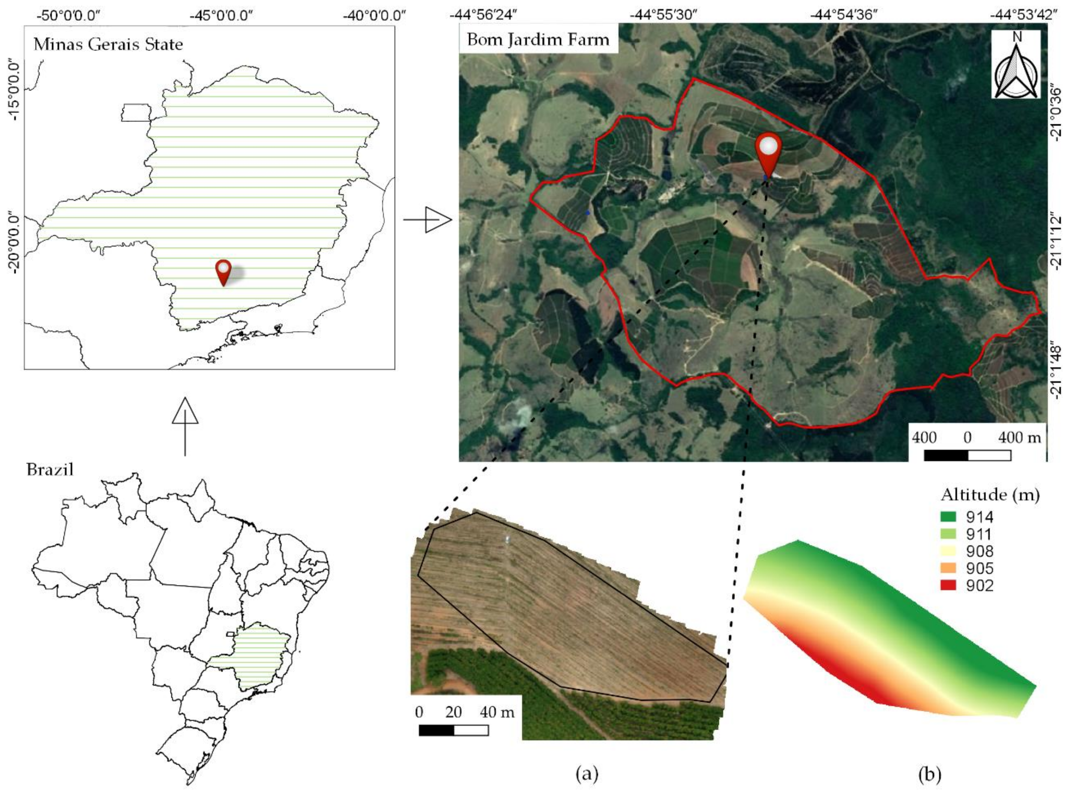
2.1. Study Area

The study area comprised 0.85 hectares in Bom Jardim farm, with altitude variations between 900 and 913.6 m (Figure 1), located in Bom Sucesso county, Minas Gerais, Brazil, under the coordinates 21°00′55.55″ S and 44°54′57.75″ W. This region is characterized by a hot and temperate climate, annual average temperatures between 20 and 22 °C, higher levels of rainfall in summer than in winter (between 1300 to 1600 mm per year), and altitude between 800 and 1000 m [21].
Coffea arabica L. coffee plantings (Catuaí Vermelho IAC 99 cultivar) were used, planted in the desired spacing of 3.5 m between rows and 0.5 m between plants. The desirable field travel speed for mechanized planting was 1.75 km/h. Planting was carried out by a planting platform coupled to a compact MF 4275 model tractor. The operation involved two auxiliary workers, one to deposit plants in the planting system and one to supply boxes on the platform, in addition to the tractor operator (Figure 2).

2.2. Obtaining Aerial Images

Images were obtained using a remotely piloted aircraft (RPA), model Phantom 4 advance (Figure 3). The images were captured by a red, green, and blue (RGB) sensor and focal aperture of 1 to get photos up to 20 megapixels.
A flight plan was inserted in the RPA mission with the goal of area recognition and data verification. Then, landing and takeoff points called “home” were defined. Flight conditions were verified following Santos et al. [22] guidelines, which ask for before-flight evaluation of the following safety factors: weather conditions; wind speed; presence of objects, posts, trees, electrical transmission towers; safe distance from airports and areas with high population density; landing and takeoff locations; and limiting factors related to the specific laws of each city/state/country.
The RPA flight mission was defined according to the following characteristics: 30 m high from the ground, 3 m.s−1 speed, and a lateral and longitudinal overlap of 80%. The pre-established flight mission was started at “home” point and returned to the same point automatically after having collected 123 images during 7 min of flight, resulting in a spatial resolution of 1.68 cm in three spectral bands, red, blue, and green. Flights were carried out at 12:00 p.m. due to low clouds and little shadow interference. Before the start of the flight, ground control points were distributed throughout the area.

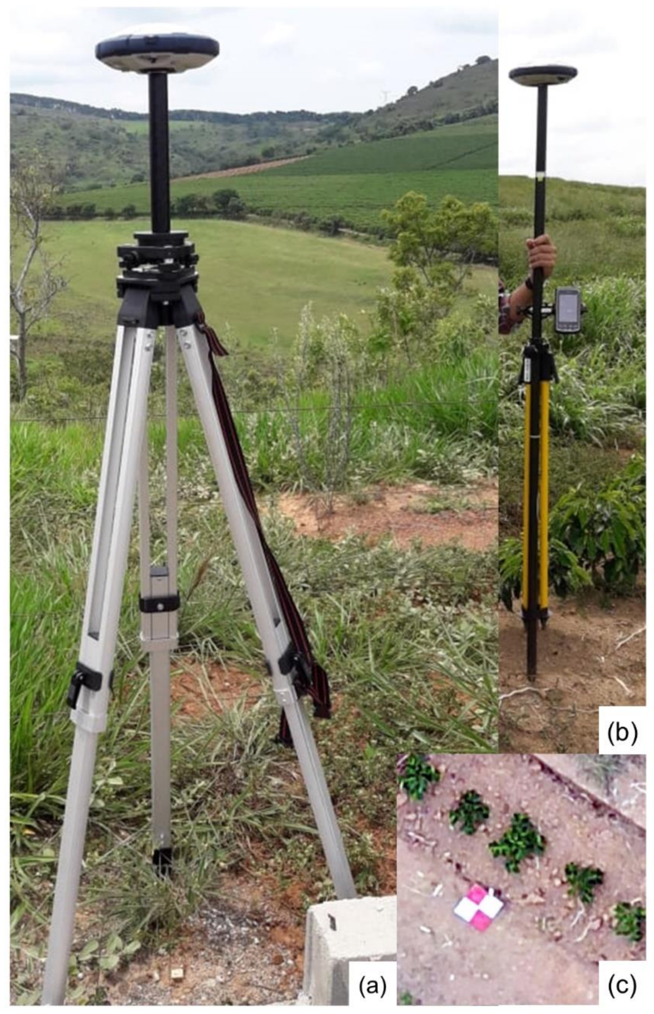
2.3. Ground Control Points—GCPs

Georeferenced ground control points can make improvements to the geometrical positioning of the orthomosaic. Some practices must be followed at the moment of GCP implantation. In this case, 13 points were tracked in the field, in a mesh form, following Rangel et al. [23] observations. The GCPs were implemented from georeferenced coordinates, collected by a pair of receivers from the Global Navigation Satellite System (GNSS), with real-time tracking performance—Real-Time Kinematic RTK mode (Figure 4a,b). Markers of 0.3 × 0.3 m (Figure 4c) were allocated in the terrain according to GCP characteristics verified in studies of [24,25].
Data collected via GNSS were processed using the EZSurv software and a digital platform from the Brazilian Institute of Geography and Statistics (IBGE). This process consisted in transforming the signals received from satellites and GNSS equipment into coordinates. Geographic coordinates (X, Y, and Z) of the RTK base were sent to IBGE and adjusted by precise point positioning (PPP) to improve accuracy. This positioning method applies orbit and clock correction to GNSS, providing positioning with global reference from anywhere in the world by a single GNSS receiver [26].

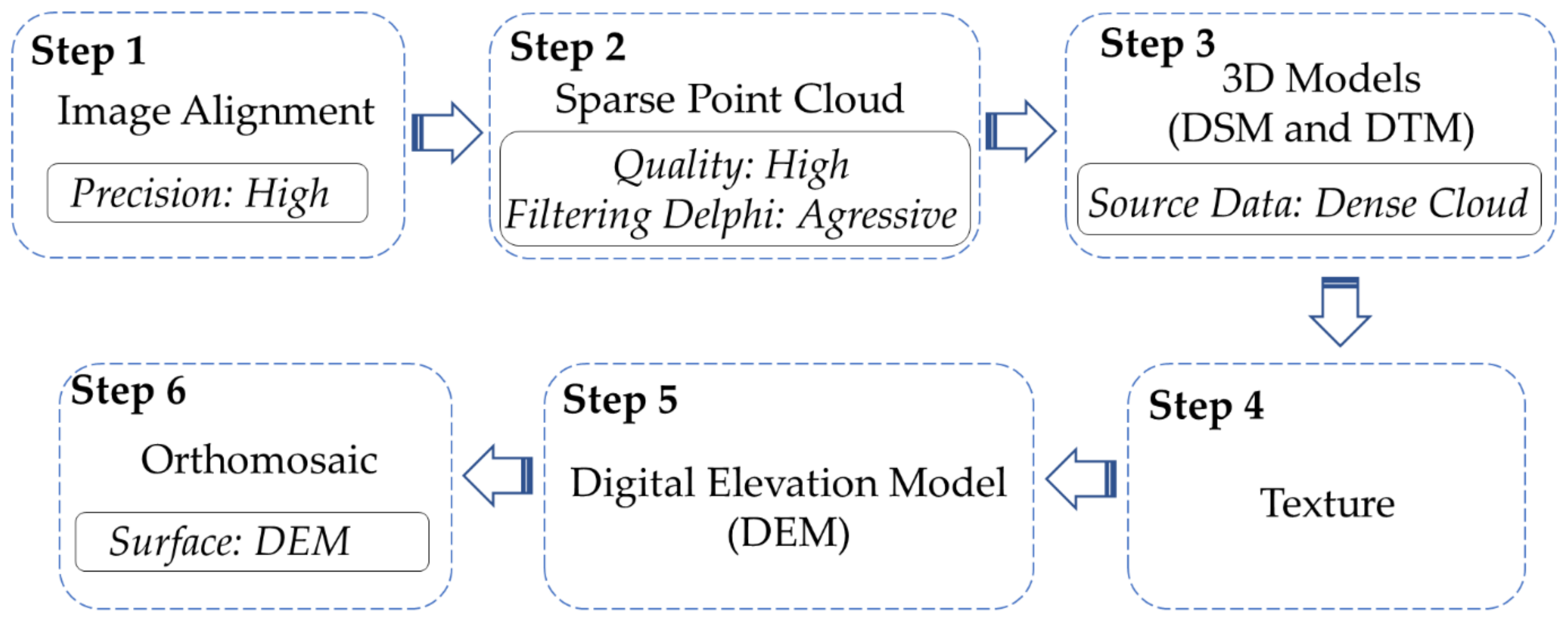
2.4. Photogrammetric Processes

Final photogrammetric products, such as orthomosaic and DTM, and aerial images require software processing based on a Structure-from-Motion (SfM) algorithm. This was done using Agisoft PhotoScan software, version 1.4.3. In terms of accuracy, this program can be considered superior when the user intends to generate orthomosaic and DTMs [27,28].
The methodology proposed by Flynn and Chapra [29] and Rusnák et al. [30] was used for image processing. This methodology is composed of six steps. Step 1: Image alignment is carried out using a photo-triangulation process and cloud generation of sparse points to materialize the terrain coordinate system. Step 2: Sparse points’ cloud generated in the previous step is densified for a more detailed representation of the mapped area. It was also referred to local coordinate system SIRGAS 2000 Zone 23S. Step 3: A three-dimensional model is built, that accurately represents mapped terrain. For this step, the Digital Surface Model (DSM) and Digital Terrain Model (DTM) are created. DTM was obtained only after filtering point clouds. Step 4: Texture is applied to the model obtained in the previous step to improve visual appearance and distinction between objects. Step 5: Digital elevation model creation (DEM). The products generated are a two-dimensional raster representation of DSM and DTM. Step 6: Orthomosaic is generated at this stage. Parameters used for image processing are shown in the flowchart (Figure 5).
After the processing step, the images were georeferenced to increase accuracy. Image processing using SFM algorithms and GCPs applications for image georeferencing contributes to reducing vertical and horizontal errors [31]. At this stage, the points collected and georeferenced to each target on the ground are inserted into the image target, generating a mean square error (RMSE). RMSE is commonly used to express numerical accuracy results and has the advantage of presenting values of errors in some dimensions of the analyzed variable [32]. In the study, an accuracy check was considered in order to generate the RMSE data. This approach consists of validating the adjusted coordinates using independent georeferenced points. Thus, each independent coordinate served as support to the studied GCP. The calculations for obtaining RMSExyz errors performed by PHOTOSCAN are presented in Equation (1).
RMSE XYZ = i = 1 n [ ( X Oi X GNSSi ) 2 + ( Y Oi Y GNSSi ) 2 + ( Z Oi Z GNSSi ) 2 n
where:
-
n is the number of GCPs.
-
XOi, YOi, and ZOi are, respectively, X, Y, and Z coordinates measured in orthophoto.
-
XGNSSi, YGNSSi, and YGNSSi are, respectively, X, Y, and Z coordinates measured in field by receivers GNSS.
Table 1 shows GCPs processing errors at each adjusted point. This table shows the minimum precision parameter for the adjustment between the photogrammetric and geodetic coordinates (Accuracy_X/Y/Z_ (m)). This value is a software default. In addition, it shows the processing results: the distance between the points obtained by photogrammetry and by GNSS receivers on each coordinate, Error_ (m), X_error (m), Y_error (m), and Z_error (m).
From the georeferenced scenes, digital elevation model data were used to create the slope map. Vegetation was removed by soil points’ classification and a digital terrain model was created. Then, DTM data were processed in ArcGIS 10.7 software, using a tool (Surface/Slope). A slope map was generated, subdivided into five classes: 0–15%, 15–20%, 20–25%, 25–30%, and 30–40%.
The Brazilian soil classification system, formulated by Brazilian Agricultural Research Corporation (EMBRAPA), considers flat relief slopes to be between 0% and 3%, and low slopes from 3% to 8%; moderate relief refers to the slopes between 8–20% [33]. Slope variations between 20–45% are considered to be strong undulating. Steep slopes, predominantly between 45–75%, are considered mountainous. The slope map indicates that the topographic aspects characterizing the study area can be classified as moderate relief and strong undulation.

2.5. Data Collection and Statistical Analysis

Plant counting was the first step to the planting performance analysis. In order for plants to be counted in each slope classification area, a point file was created from the georeferenced location of each plant in the study area (Figure 6a).
Samples of spacing between planting lines and between plants in line were collected from the slope map (Figure 6b). Slope data were exported to the Computer-Aided Design (CAD) platform. Three samplings were performed for each slope level, as shown in the black rectangles in Figure 6b. From this conformation, 120 images of distances between plants were obtained in each rectangle for the category “distances between plants”. To obtain the category “spacing between planting lines”, 30 images of distance between the planting lines were collected in each rectangle. Thus, 360 plants were analyzed in the category “distances between plants” and 90 plants for the analysis of line spacing at each level of slope.
Control charts were used to identify erroneous points in the alignment of planting and the spacing between plants, which may be related to the influence of the slope. Each level of slope was considered an experimental treatment (independent variable) and to increase statistical reliability, three repetitions were applied at each level as shown in the rectangles in Figure 6b.
In SPC chart analysis, values found within mobile range limits are considered acceptable. The control charts are composed of three lines, central line (mean), upper control limit (UCL), and lower control limit (LCL). In order to avoid negative values in the lower control limit (LCL), this was considered a null value (LCL = 0, for individual values chart and LCL = 1 for mobile amplitude chart). The average line and limits of control graphs were estimated according to Equations (2)–(4), proposed by Molnau et al. [34].
Center line (X) = c4 (ni)
UCL = σ + k (c5(ni)/c4(ni))s
LCL = σ − k (c5(ni)/c4(ni))s
where:
  • c4 and c5: values from a table
  • ni: size of the ith subgroup
  • k: parameter that is specified for Test 1 of the tests for special causes, 1 point > K standard deviations from center line. By default, k = 3.
  • σ: estimated standard deviation, which depends on the options chosen.
SPC analyses were performed using Statistics 7 software. Slope data from CAD vectors were tabulated in electronic spreadsheets and inserted in Statistics 7. Charts resulting from SPC analyses were X BAR S type, presented in two ways: (a) considering the average of the samples, or (b) considering the sample’s standard deviation, known as range graph.
Variance analyses (ANOVA) were performed by a completely randomized experimental design, in the following setup. Independent variable: slope % (in levels: 0–15, 15–20, 20–25, 25–30, 30–40). Dependents variables: spacing between plants and spacing between planting lines. Replication number: three regions selected randomly for each independent variable (slope levels). SISVAR 5.6 software was used for statistical procedures when starting an exploratory analysis (descriptive statistics) to verify data normality and occurrence or need to transform for normalization. Once normality was verified, a variance analysis (ANOVA) of one-way type was performed. The F test was used, and then the Tukey test was performed at a 5% probability of error.

3. Results

3.1. Plant Distribution

Plant distribution efficiency at each slope level is shown in Table 2. The best result found for planting distribution was in the 30–40% range. The transplanted quantity was 98.78% of the projected quantity, which may be related to the low speed used in planting on steep slopes.
The lowest efficiency in planting distribution was found in the 20–25% range. As shown in Table 2, only 92.11% of projected plants were distributed in this slope range.

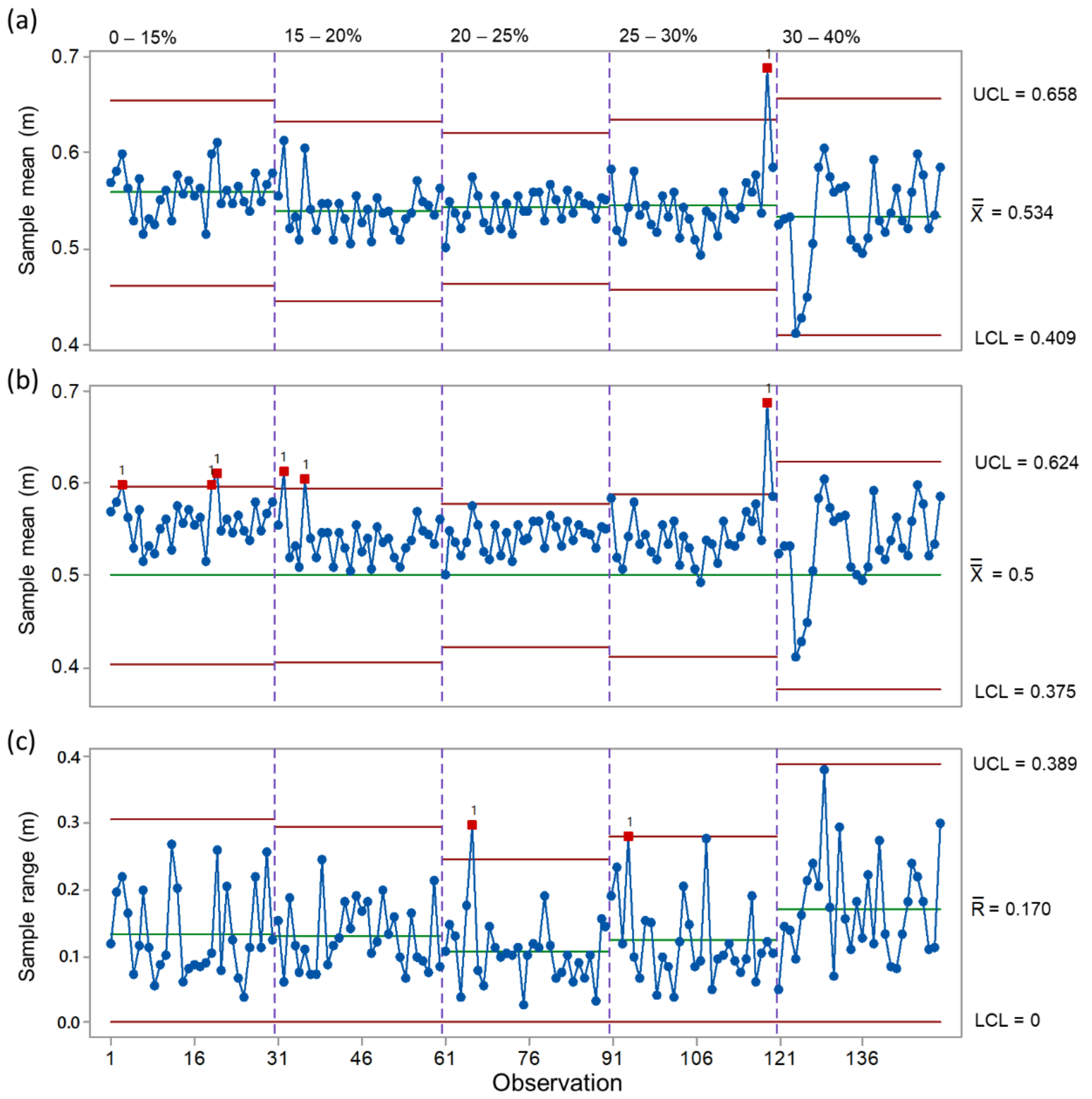
3.2. Spacing between Plants

The statistical results of plant distribution for analysis of plant space in a row are shown in Table 3. Even though the probability test ‘test-p’ shows, at a 5% probability of error, that averages do not differ from each other, the alternative hypothesis obtained in the statistical model indicates that one of the averages may be different, justifying the performance of the Tukey test. The treatment that possibly differed from the others was shown by the Tukey test.
As a result, pruning operations were directly affected when the equipment was adjusted concerning plant height. Figure 7 presents the results of Tukey’s test analyses. Filters that represent the treatments with significant errors at 5% of probability are in red.
Verification of errors found in the average tests shows the influence of the slope. Therefore, for a better understanding of the slope effect, the data were inserted in quality control graphs (Figure 8), in which they showed variations of the samples (blue line), calculated average error X ¯ , projected average error X ¯ (0.5 m), and standard deviation R ¯ (green line) on the spacing samples between plants in the planting line. The red points found outside the UCL and LCL limits comprise errors in the process that reduced the quality of planting.

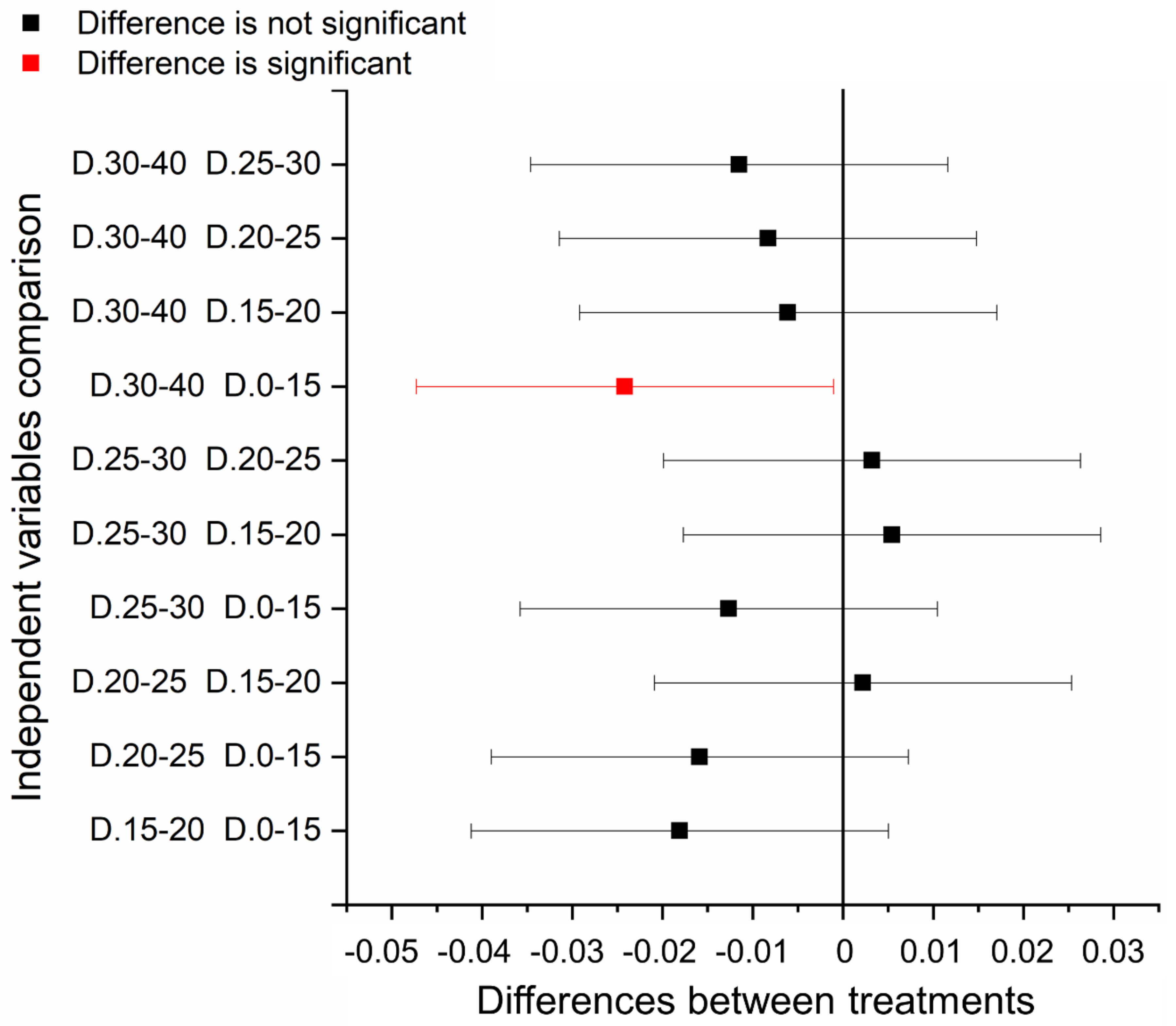
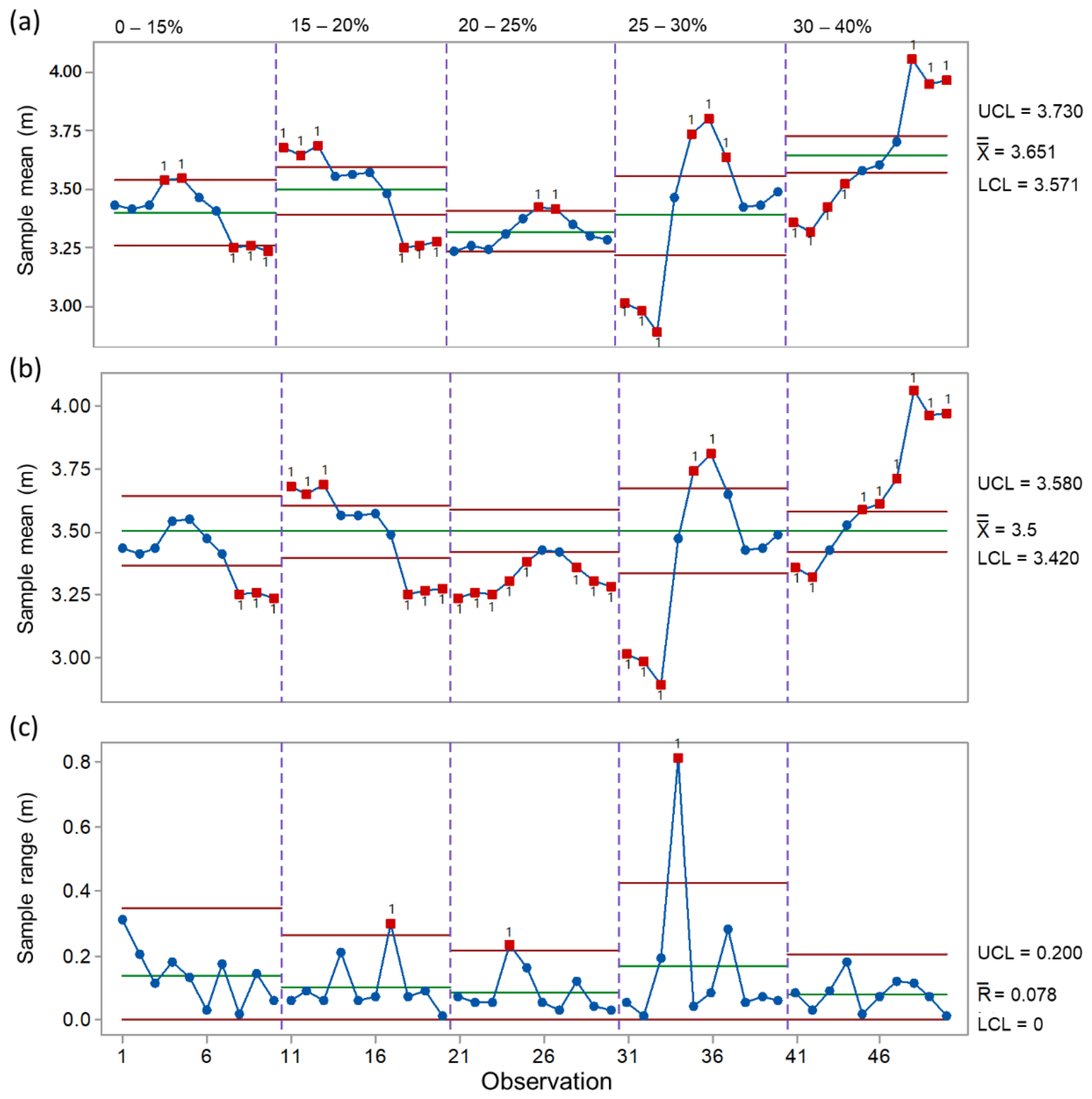
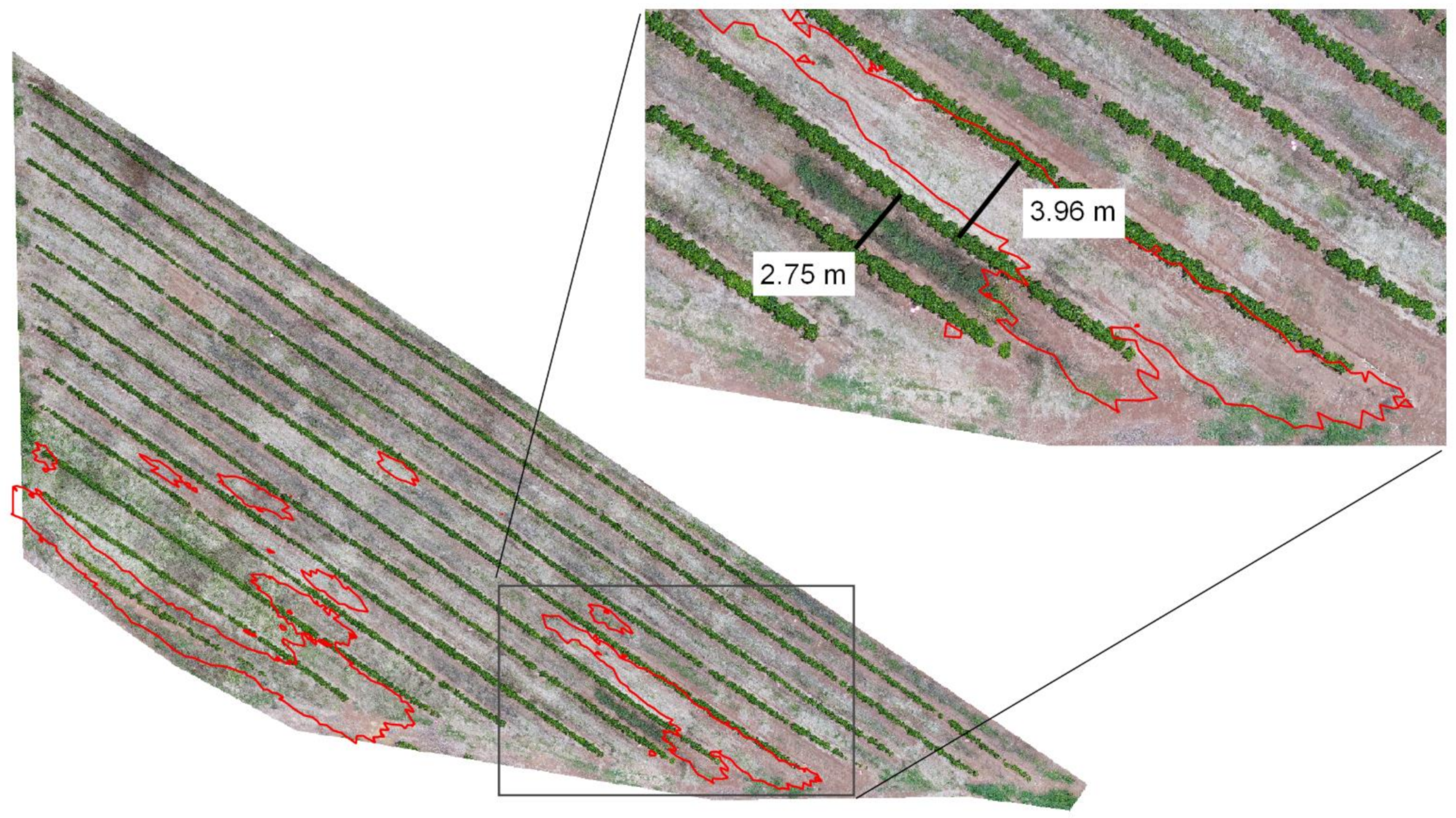
3.3. Spacing between Planting Rows

Statistical results of plant distribution are shown in Table 4. When analyzing the spacing between planting rows, significant differences between treatments in slope ranges analyzed using Tukey’s test were found. These results prove that some slopes influenced distances between planting rows.
Results of spacing between planting rows indicate that the most suitable treatment to initial planting planning was found in 15–20% slopes (Table 4), for which it presented a 3.49 m average value, a result very close to the projected distance (3.5 m). The most distant results from the desired planting were found at an average of 20–25% slope. In this slope range, the spacing between planting rows showed a 3.32 m average, differing from the 15–20% and 30–40% slopes in average tests at 5% error probability. From the results in Table 2, it is evident that when a semi-mechanized planting is carried out on 0–15%, 15–20%, and 25–30% slopes, the spacing between planting rows does not present a significant difference.
Average tests applied to rows spacing variables are presented in Figure 9. It is possible to note that the 30–40% slope showed significant differences when compared to 0–15%, 20–25%, and 25–30% slopes. It is worth mentioning that although the 30–40% slope was significantly different from the 15–20% slope, the difference in these treatments was at a statistical significance limit.
Error verification in the average tests shows that there was a slope influence. However, for a better understanding, the control charts for the variations of distances in planting rows are presented in Figure 10. Average sample variation (blue line), calculated average error X ¯ , projected average error X ¯ (0.5 m), and standard deviation R ¯ (green line) for planting line spacing samples are shown. The red dots found outside the UCL and LCL limits comprise errors in the process that reduced the quality of planting.

4. Discussion

4.1. Plant Distribution

Inefficient planting distributions in sloping environments are related to daily planting productivity. The implemented slowdown on high slopes causes operators to accelerate the operation on mild slopes to maintain daily planting average. This occurrence may have influenced the planting performed on the slopes 20–25% which presented low performance. According to Tavares et al. [35], on the steepest slopes, operations require that the operator makes continuous gear changes to reduce the accident risk, which leads to an operation speed decrease.
The planting system can distribute fewer plants than expected. Differences found in the plants’ number distributed can interfere with crop implanting costs, as investments made by the producer are calculated for planned cultivation. Coffee (Coffea arabica)’s production cost for a projected population of plants in a semi-mechanized system is BRL 10,110.55 ha−1 [36]. Analyses of implantation systems of a coffee crop [37] state that the semi-mechanized planting system has operating costs of around BRL 580.97 ha−1. These studies express data for a projected population of plants based on data presented in Table 2; plant distribution interference in costs is highlighted.
It is important to note that just observing the data in Table 2 is not enough to affirm that operation has occurred with expected quality, that is, ensuring the plants were transplanted in their proper location. Even though quantities may be correct, the coffee plant needs to be deposited with correct spacing, both between-row planting and between plants, in order to ensure appropriate crop development and a crop optimization of management operations.

4.2. Spacing between Plants

From the distances between plants in the planting row, shown in Table 3, it is possible to note that planting on all slopes presented average values above the projected. The effect of different spacing on coffee crop development is very evident. When evaluating the consequences of spacing plants reduction in planting row, Pereira et al. [38] showed, by regression analysis, that for each meter added in spacing between plants, the obtained plants are 0.53 m lower than expected height. Variations in spacing between plants in planting rows, caused by slope levels, can make plants’ heights uneven.
According to data presented in Figure 7, the slopes 0–15% and 30–40% are different from each other according to Tukey’s test. For these slopes, the difference in averages of spacing between plants in planting row was 0.024 m. Although a low difference was found in plant spacing, it is essential to note that this type of error is cumulative. Therefore, over long planting distances, this error can be relevant.
Variations in the process can be explained by Martins and Laugeni [39], who classified variations in sample points into two causes: common and special. The authors pointed out that common causes are intrinsic to the process, and special causes can be corrected by employing adjustments. According to Hadian and Rahimifard [40], the “out of control” process occurs when points on the control chart move outside the upper or lower limit. With that, the process shifts from a projected average over some periods of time.
As shown in Figure 8a, all average spacing between plants in the planting line was within the calculated limit (UCL and LCL), except for one point found on a 25–30% slope that was outside the upper control limit. The point found outside the upper limit was considered “special causes” and may be related to failures in the distribution of the plant on the line. Figure 8 represents a moving average, in which case the errors can be mitigated, as this configuration is guided by the set of data entered.
When analyzing Figure 8b, we notice that when setting the average at the desired level, the set of averages is then presented above the projected line. In Figure 8b, variations in the spacing between plants in the planting line are seen as “common causes” on slopes of 20–25% and 30–40% and “special causes” on slopes of 0–15%, 15–20%, and 25–30%. For all slopes, points above the projected average (0.5 m) can also be observed, even with common causes, plantings on 30–40% slopes present a high variation between sampled points. It may have occurred due to lateral platform movement, with diagonal distancing.
In quality studies on mechanized soil tilling and coffee planting, Silva et al. [41] concluded that, even at a 5% slope, errors in planting spacing could occur in planting rows. The authors observed variations of special causes in all processes, with possible sudden changes in direction by the operator during operation. These changes can occur due to planting conditions like terrain type, tractor skating, slope, and plant replenishment on the platform, among others.
Standard deviations of samples are presented in the process control chart (Figure 8c). In the range between 20–30% slope, points outside the upper limit can be observed. High variations in standard deviation can be related to planting failures, that is, planting not deposited in the furrow, generating spacing between plants in the planting row of around 1 m.

4.3. Spacing between Planting Rows

Errors in spacing between planting rows can interfere in plants’ number, and consequently, error accumulation between rows can suppress or add planting rows. In a hypothetical situation, 1 hectare of coffee planting with 3.5 m projected spacing creates 28 rows of 100 m. This research shows that plantings carried out in that same area with a semi-mechanized system in the 20–25% slope range were transplanted. When carrying out planting operations at the 30–40% slope range, only 27 rows are planted, due to spacing reduction in this slope range.
All the slopes evaluated showed special causes errors, and for slopes above 25%, errors increased even more, allowing for observation of sample points exceeding the upper and lower limits. These data reinforce the direct effect of the slope on planting quality, especially about the spacing between planting rows.
Coffee plantations implanted in Minas Gerais, Brazil are present in varying levels of slope. However, most of them, around 75%, are installed on slopes of less than 20%, allowing the use of mechanized management [42]. The choice of regions below 20% slope can facilitate the operation and lead to minor errors; as seen in Figure 10, on slopes above 25%, there are points outside the limits drastically alternating between UCL and LCL. This is because the operator tried to compensate for previous line errors. The same was found in research carried out by Rezende [43], which considered slopes below 20% to be suitable for mechanization.
Slopes above 25% showed points of special causes errors, that is, outside the upper and lower limits. The presence of these special causes errors may have occurred due to the corrective action of the operator trying to adjust spacing errors. The average distance between plants was high at some locations and low at others. The occurrence of these errors may be related to planting platform stability, which can be aggravated by the increase in steepness of the slope. This result can be compared to the Höfig [44] study which presents some data on the ability to mechanize coffee planting in sloping regions. They showed that between 0–5% is extremely suitable, 5.1–10% very suitable, 10.1–15% suitable, 15.1–20% moderately suitable, and above 20% is not recommended.
The control chart (Figure 10b) shows the slope influence on distance variations between planting rows. When comparing the changes observed in the field with the desired 3.5 m spacing, all slopes evaluated were outside the control chart limits. Therefore, the erroneous points noted in the control chart are considered special causes errors. Consequently, process improvements can correct these errors. In mechanized operations, unwanted variations in the spacing between planting rows can decrease the machine’s performance.
Adjustment of equipment used for the management of fertility in coffee-growing is carried out taking into account the planned spacing during the planting operation. In the planting carried out on 30–40% slopes, the average spacing between rows was 3.65 m, above the desired average (3.5 m). In this case, fertilizer distribution may not meet the necessary nutritional requirements of the plant, since, in greater spacing between planting rows, covering fertilizer can be applied outside the plant architecture, where the highest roots concentration was found. In a Kenya study, Huxley et al. [45] observed that most of the root activity was on the soil surface, on a horizontal distance between 0.1 to 0.75 m around the plant stem. This was proven by Covre et al. [46] researching root development in irrigated coffee cultivations.
In weed mowing operations, the spacing adopted by the producer determines the width of the cutting platform. This operation may be subject to the more significant influence of errors in spacing between rows, as the platform width of conventional cutters cannot be adjusted, causing the producer to acquire cut implements according to projected spacing. Research by Guerra et al. [47] considers spacing between lines used in a mechanized system of coffee cultivation of between 3.8 and 4 m. However, coffee crops can be fully mechanized with a spacing of up to 3.5 m.
To reinforce the previous argument, in the experimental field of this research, we found agricultural management barriers, with the goal to clear weeds, as shown in Figure 11. In regions where the mechanized system performed the cutting operations, it was necessary for a worker to brush manually or semi-mechanically.
The weed cleaning operation carried out in regions with a slope of 30–40% was interrupted by errors in planting (Figure 11). In this case, the increase in distance between planting rows to 3.96 m interfered with the acing of the next row, which presented 2.75 m between rows. This phenomenon hindered the passage of weed removal implement. For higher yields in weed clearing management, the operation is performed with the implement of the row width; in this way, weeds get cut in a single pass.
Pesticide applications are susceptible to interference when there are errors in the spacing between planting lines. According to Júnior et al. [48], one way of calibrating the sprayer is to calculate the volume amount to be sprayed. Multiplying the displacement of the mechanized set in 50 m by the desired spacing between lines will result in the necessary pesticide amount per hectare. Following the errors’ evaluation in planting, spraying should be corrected taking into account the actual spacing, and then the correct pesticide amount should be applied. This would increase the pesticide application efficiency, since the calculated volume of pesticide is applied as a function of the projected distance (3.5 m).
On 20–25% and 30–40% slopes, variations in average distances (3.32 and 3.65 m) around the projected line spacing (3.5 m) can interfere in leaf application uniformity. Santinato et al. [49] demonstrate that, whether to control fungal diseases or just to supply nutrients via leaf application, there is a need for a minimum amount of pesticide spray to be deposited uniformly on the plant. Therefore, for greater spacing, the applied pesticide amount could be insufficient. Inversely, pesticide amounts may be excessive in shorter distances between plants.
Regarding mechanized coffee harvesting, Santinato et al. [50] warn of the risk of this operation type on high slopes, concluding that for slopes above 20%, mechanized harvesting requires 21.6% more time to be carried out than in lower slopes. Moreover, alignment errors can extend harvest time even further, because they demand more maneuvers in operation. For mechanized harvesting operations, Silva and Salvador [51] show the linespacing influence in management with tractor-drawn harvester and define a 3.5 m minimum spacing between planting rows, and draw attention to well-aligned plants. This study found spacings that did not meet requirements for tractor-drawn harvester handling. The slopes 0–15%, 20–25%, and 25–30% showed, respectively, spacing between planting rows of 3.34, 3.32, and 3.39 m.
Given the above, it is evident that plant alignment errors influence all management operations after planting. It is clear that alignment improvements contribute to better operational yields of the coffee crop management in steep slopes.

5. Conclusions

Semi-mechanized system planting carried out on a 30–40% slope showed better planting distribution. In contrast, planting of coffee on 20–25% slopes caused the lowest efficiency in planting distribution.
Differences in plant spacing in the planting rows on 0–15% and 30–40% slopes were significant. Differences found in distances between plants can be related to factors such as speed, planting system efficiency, planting consistency, and worker experience. This research shows that plant alignment errors influence all management operations after planting and that alignment improvements contribute to better operational yields of the coffee crop management in steep slopes.

Author Contributions

Conceptualization, L.S.S. and G.A.e.S.F.; methodology, J.P.B.C. and R.d.O.F.; software, D.B.M.; validation, L.S.S., G.A.e.S.F. and R.d.O.F.; formal analysis, D.B.M. and G.R.; investigation, M.S.S.; resources, M.V. and L.C.; data curation, D.S.; writing—original draft preparation, L.S.S.; writing—review and editing, G.A.e.S.F. and L.S.S.; visualization, G.R.; supervision, J.P.B.C.; project administration, G.A.e.S.F.; funding acquisition, G.A.e.S.F., G.R., D.S., L.C. and M.V. All authors have read and agreed to the published version of the manuscript.

Funding

This research was funded by the Embrapa Café—Consórcio Pesquisa Café, project approved n◦ 234/2019, the National Council for Scientific and Technological Development (CNPq), the Coordination for the Improvement of Higher Education Personnel (CAPES), the Federal University of Lavras (UFLA), and University of Firenze (UniFI).

Institutional Review Board Statement

Not applicable.

Informed Consent Statement

Not applicable.

Data Availability Statement

Data sharing not applicable.

Acknowledgments

The authors would like to thank Bom Jardim farm.

Conflicts of Interest

The authors declare no conflict of interest.

References

  1. Belan, L.L.; Junior, W.C.d.J.; Souza, A.F.; Zambolim, L.; Filho, J.C.; Barbosa, D.H.S.G.; Moraes, W.B. Management of coffee leaf rust in Coffea canephora based on disease monitoring reduces fungicide use and management cost. Eur. J. Plant Pathol. 2020, 156, 683–694. [Google Scholar] [CrossRef]
  2. Baitelle, D.C.; Freitas, S.D.J.; Vieira, K.M. Feasibility and Economic Risk of Programmed Pruning Cycle in Arabic Coffee Feasibility and Economic Risk of Programmed Pruning Cycle in Arabic Coffee. J. Exp. Agric. Int. 2018. [Google Scholar] [CrossRef] [Green Version]
  3. Cunha, J.P.B.; Silva, F.M.; Dias, R.E.B.A. Eficiência de campo em diferentes operações mecanizadas na cafeicultura. Coffee Sci. 2016, 11, 76–86. [Google Scholar]
  4. Fernandes, A.L.T.; Partelli, F.L.; Bonomo, R.; Golynski, A. A moderna cafeicultura dos cerrados brasileiros. Pesqui. Agropecuária Trop. 2012, 42, 231–240. [Google Scholar] [CrossRef]
  5. Silva, J.A.R.; Oliveira, G.G.; Júnior, C.E.; Melo Costa, A.B.; Silva, C.P.C.; Gabriel, F.F.P. Occupational noise level in mechanized and semimecanized harvest of coffee fruits. Coffee Sci. 2018, 13, 448–454. [Google Scholar] [CrossRef]
  6. Aparecido, L.E.d.O.; Souza, I.T.d.; Miranda, G.R.B.; Moraes, J.R.d.S.C.; Moraes-Oliveira, A.F.; Paula, F.V. Tipos de plantio e fertilizante biológico no cafeeiro em função do índice térmico. Coffee Sci. 2017, 12, 307–315. [Google Scholar] [CrossRef]
  7. Marchi, E.C.S.; Campos, K.P.; Corrêa, J.B.D.; Guimarães, R.J.; Souza, C.A.S. Sobrevivência de mudas de cafeeiro produzidas em sacos plásticos e tubetes no sistema convencional e plantio direto, em duas classes de solo. Ceres 2003, 50, 407–416. [Google Scholar]
  8. Gimenes, G.R.; Oliveira, R.B.; Silva, A.F.; Reis, L.C.; Reis, T.E.S. Mapping of slopes for the operation of agricultural harvesters in Bandeirantes Municipality (PR). Semin. Agrar. 2017, 38, 97–107. [Google Scholar] [CrossRef] [Green Version]
  9. Dubbini, M.; Curzio, L.I.; Campedelli, A. Digital elevation models from unmanned aerial vehicle surveys for archaeological interpretation of terrain anomalies: Case study of the Roman castrum of Burnum (Croatia). J. Archaeol. Sci. Rep. 2016, 8, 121–134. [Google Scholar] [CrossRef] [Green Version]
  10. Akturk, E.; Altunel, A.O. Accuracy assesment of a low-cost UAV derived digital elevation model (DEM) in a highly broken and vegetated terrain. Meas. J. Int. Meas. Confed. 2019, 136, 382–386. [Google Scholar] [CrossRef]
  11. Uysal, M.; Toprak, A.S.; Polat, N. DEM generation with UAV Photogrammetry and accuracy analysis in Sahitler hill. Meas. J. Int. Meas. Confed. 2015, 73, 539–543. [Google Scholar] [CrossRef]
  12. Piras, M.; Taddia, G.; Forno, M.G.; Gattiglio, M.; Aicardi, I.; Dabove, P.; Russo, S.L.; Lingua, A. Detailed geological mapping in mountain areas using an unmanned aerial vehicle: Application to the Rodoretto Valley, NW Italian Alps. Geomat. Nat. Hazards Risk 2017, 8, 137–149. [Google Scholar] [CrossRef]
  13. Zhang, C.; Kovacs, J.M. The application of small unmanned aerial systems for precision agriculture: A review. Precis. Agric. 2012, 13, 693–712. [Google Scholar] [CrossRef]
  14. Peloia, P.R.; Milan, M.; Romanelli, T.L. Capacity of the mechanical harvesting process of sugar cane billets. Sci. Agric. 2010, 67, 619–623. [Google Scholar] [CrossRef]
  15. Zerbato, C.; Furlani, C.E.A.; Voltarelli, M.A.; Bertonha, R.S.; Silva, R.P. Quality control to seeding systems and densities in peanut crop. Aust. J. Crop Sci. 2014, 8, 992–998. [Google Scholar]
  16. Hrvačić, I. Design and implementation of SPC systems in defense industry manufacturing process. Period. Eng. Nat. Sci. 2018, 6, 27–40. [Google Scholar] [CrossRef] [Green Version]
  17. Toledo, A.; Tabile, R.A.; Silva, R.P.; Furlani, C.E.A.; Magalhães, S.C.; Costa, B.O. Caracterização das perdas e distribuição de cobertura vegetal em colheita mecanizada de soja. Eng. Agric. 2008, 28, 710–719. [Google Scholar] [CrossRef]
  18. Noronha, R.H.d.F.; Oliveira, M.F.; Mendes, A.L.; Damasceno, A.F.; Zerbato, C.; Furlani, C.E.A. Application of signal correction for sphenophorus levis control and higher quality production in mechanized harvesting of sugarcane ratoon. Aust. J. Crop Sci. 2019, 13, 1936–1942. [Google Scholar] [CrossRef]
  19. Chinchilla, S.R.A.; Silva, Ê.F.d.F.; Almeida, C.D.G.C.; Silva, A.O.; Santos, P.R. Statistical process control in the assessment of drip irrigation using wastewater. Eng. Agric. 2018, 38, 47–54. [Google Scholar] [CrossRef] [Green Version]
  20. Cunha, J.P.B.; Silva, F.M.; Andrade, E.T.; Barros, M.M. De Parameters of operational performance of soil preparation and semi- mechanized transplantation of coffee seedling. Eng. Agric. 2018, 38, 910–917. [Google Scholar]
  21. Alvares, C.A.; Stape, J.L.; Sentelhas, P.C.; De Moraes Gonçalves, J.L.; Sparovek, G. Köppen’s climate classification map for Brazil. Meteorol. Z. 2013, 22, 711–728. [Google Scholar] [CrossRef]
  22. Santos, L.M.D.; Ferraz, G.A.S.; Andrade, M.T.; Santana, L.S.; Barbosa, B.D.S.; Maciel, D.T.; Rossi, G. Analysis of flight parameters and georeferencing of images with different control points obtained by RPA. Agron. Res. 2019, 17, 2054–2063. [Google Scholar] [CrossRef]
  23. Rangel, J.M.G.; Gonçalves, G.R.; Pérez, J.A. The impact of number and spatial distribution of GCPs on the positional accuracy of geospatial products derived from low-cost UASs. Int. J. Remote Sens. 2018, 39, 7154–7171. [Google Scholar] [CrossRef]
  24. Liba, N.; Berg-Jürgens, J. Accuracy of orthomosaic generated by different methods in example of UAV platform MUST Q. IOP Conf. Ser. Mater. Sci. Eng. 2015, 96, 012041. [Google Scholar] [CrossRef]
  25. Santana, L.S.; Ferraz, G.A.E.S.; Marin, D.B.; Barbosa, B.D.S.; Santos, L.M.; Ferraz, P.F.P.; Conti, L.; Camiciottoli, S.; Rossi, G. Influence of flight altitude and control points in the georeferencing of images obtained by unmanned aerial vehicle. Eur. J. Remote Sens. 2021, 54, 59–71. [Google Scholar] [CrossRef]
  26. Grinter, T.; Roberts, C. Precise Point Positioning: Where are we now? In Proceedings of the IGNSS Symposium 2011, Sydney, Australia, 15–17 November 2011; pp. 1–15. [Google Scholar]
  27. Sona, G.; Pinto, L.; Pagliari, D.; Passoni, D.; Gini, R. Experimental analysis of different software packages for orientation and digital surface modelling from UAV images. Earth Sci. Inform. 2014, 7, 97–107. [Google Scholar] [CrossRef]
  28. Dietrich, J.T. Riverscape mapping with helicopter-based Structure-from-Motion photogrammetry. Geomorphology 2016, 252, 144–157. [Google Scholar] [CrossRef]
  29. Flynn, K.; Chapra, S. Remote sensing of submerged aquatic vegetation in a shallow non-turbid river using an unmanned aerial vehicle. Remote Sens. 2014, 6, 12815–12836. [Google Scholar] [CrossRef] [Green Version]
  30. Rusnák, M.; Sládek, J.; Kidová, A.; Lehotský, M. Template for high-resolution river landscape mapping using UAV technology. Meas. J. Int. Meas. Confed. 2018, 115, 139–151. [Google Scholar] [CrossRef]
  31. Tonkin, T.N.; Midgley, N.G. Ground-control networks for image based surface reconstruction: An investigation of optimum survey designs using UAV derived imagery and structure-from-motion photogrammetry. Remote Sens. 2016, 8, 786. [Google Scholar] [CrossRef] [Green Version]
  32. Hallak, R.; Pereira Filho, A.J. Metodologia para análise de desempenho de simulações de sistemas convectivos na região metropolitana de São Paulo com o modelo ARPS: Sensibilidade a variações com os esquemas de advecção e assimilação de dados. Rev. Bras. Meteor. 2011, 26, 591–608. [Google Scholar] [CrossRef] [Green Version]
  33. Santos, H.G.; Jacomine, P.K.T.; Anjos, L.H.C.; Oliveira, V.Á.; Lumbreras, J.F.; Coelho, M.R.; Almeida, J.A.; Araujo Filho, J.C.d.; Oliveira, J.B.; Cunha, T.J.F. Sistema Brasileiro de Classificação de Solos; Embrapa Solos Rua Jardim Botânico: Rio de Janeiro, Brazil, 2018; ISBN 978-85-7035-198-2. [Google Scholar]
  34. Molnau, W.E.; Montgomery, D.C.; Runger, G.C. Statistically constrained economic design of the Multivariate Exponentially Weighted Moving Average control chart. Qual. Reliab. Eng. Int. 2001, 17, 39–49. [Google Scholar] [CrossRef]
  35. Tavares, T.d.O.; Silva, R.P.; Santinato, F.; Santos, A.F.; Paixao, C.S.S.; Silva, V.d.A. Operational performance of the mechanized picking of coffee in four soil slope. Afr. J. Agric. Res. 2016, 11, 4857–4863. [Google Scholar] [CrossRef] [Green Version]
  36. Alves, E.L.; Pereira, F.A.C.; Dalchiavon, F.C. Potencial econômico da utilização de micro-terraceamento em lavouras de café: Um estudo de caso. Rev. IPecege 2017, 3, 24–38. [Google Scholar] [CrossRef] [Green Version]
  37. Cunha, J.P.B.; Silva, F.M.d.; Andrade, F.; Machado, T.d.A.; Batista, F.A. Análise técnica e economica de diferentes sistemas de transplantio de café (Coffea arabica L.). Coffee Sci. 2015, 10, 289–297. [Google Scholar]
  38. Pereira, S.P.; Bartholo, G.F.; Baliza, D.P.; Sobreira, F.M.; Guimarães, R.J. Crescimento, produtividade e bienalidade do cafeeiro em função do espaçamento de cultivo. Pesqui. Agropecu. Bras. 2011, 46, 152–160. [Google Scholar] [CrossRef]
  39. Martins, P.G.; Laugeni, F.R. Administração da Produção; Editora Saraiva: São Paulo, Brazil, 2005. [Google Scholar]
  40. Hadian, H.; Rahimifard, A. Multivariate statistical control chart and process capability indices for simultaneous monitoring of project duration and cost. Comput. Ind. Eng. 2019, 130, 788–797. [Google Scholar] [CrossRef]
  41. Silva, R.P.; Voltarelli, M.A.; Cassia, M.T.; Vidal, D.O.; Cavichioli, F.A. Qualidade das operações de preparo de solo e transplantio mecanizado de mudas de café. Coffee Sci. 2014, 9, 51–60. [Google Scholar]
  42. Bernardes, T.; Moreira, M.A.; Adami, M.; Rudorff, B.F.T. Physic-environmental diagnosis of coffee crop in the state of Minas Gerais, Brazil. Coffee Sci. 2012, 7, 139–151. [Google Scholar] [CrossRef]
  43. Rezende, F.A. Determinação das Áreas Cafeeiras Mecanizáveis no sul de Minas Gerais Com Cenários Para a Colheita. Master’s Thesis, Federal University of Lavras, Lavras, Brazil, 2008. [Google Scholar]
  44. Höfig, P.; Araujo-Junior, C.F. Classes de declividade do terreno e potencial para no estado do paraná. Coffee Sci. 2015, 10, 195–203. [Google Scholar]
  45. Huxley, P.A.; Patel, R.Z.; Kabaara, A.M.; Mitchell, H.W. Tracer studies with 32P on the distribution of functional roots of Arabica coffee in Kenya. Ann. Appl. Biol. 1974, 77, 159–180. [Google Scholar] [CrossRef]
  46. Covre, A.M.; Partelli, F.L.; Gontijo, I.; Zucoloto, M. Distribuição do sistema radicular de cafeeiro conilon irrigado e não irrigado. Pesqui. Agropecu. Bras. 2015, 50, 1006–1016. [Google Scholar] [CrossRef] [Green Version]
  47. Guerra, A.; Rocha, O.; Rodrigues, G.; Sanzonowicz, C.; Mera, A.; Cordeiro, A. Comportamento de Três Cultivares de Café Submetidas a Diferentes Espaçamentos Entre Linhas e Regimes Hídricos no Cerrado; Embrapa Solos Rua Jardim Botânico: Rio de Janeiro, Brazil, 2007. [Google Scholar]
  48. Júnior, J.M.D.S.; Ruas, R.A.A.; Silva, C.D.; Faria, V.R.; Filho, A.C.; Vieira, L.C. Determination of spray volume index for culture of coffee. Coffee Sci. 2017, 12, 82–90. [Google Scholar] [CrossRef]
  49. Santinato, F.; Ruas, R.A.A.; Silva, C.D.; Silva, R.P.; Gonçalves, V.A.R.; Júnior, J.M.D.S. Deposição da calda de pulverização em diferentes volumes vegetativos de Coffea arabica L. Coffee Sci. 2017, 12, 69. [Google Scholar] [CrossRef]
  50. Santinato, F.; Silva, R.P.; Silva, V.d.A.; Silva, C.D.; Tavares, T.d.O. Mechanical Harvesting of Coffee in High Slope. Rev. Caatinga 2016, 29, 685–691. [Google Scholar] [CrossRef] [Green Version]
  51. Silva, F.D.; Salvador, N. Mecanização da Lavoura Cafeeira, 55th ed.; Universidade Federal de Lavras: Lavras, Brazil, 1998. [Google Scholar]
Figure 1. Study area location, (a) scene in red, green, and blue composition (RGB) and (b) altitude map, in meters.
Agronomy 11 01224 g001
Figure 2. Planting operations, a semi-mechanized system using a platform.
Agronomy 11 01224 g002
Figure 3. Equipment used to collect images, (a) radio control and (b) remotely piloted aircraft (RPA).
Agronomy 11 01224 g003
Figure 4. Equipment used for control points georeferencing. (a) GNSS receiver (base), (b) GNSS receiver (Rover) RTK mode, (c): ground control points (GCPs).
Agronomy 11 01224 g004
Figure 5. Aerial image processing steps and respective parameters used in Agisoft Photoscan for orthomosaic generation.
Agronomy 11 01224 g005
Figure 6. Data collection for SPC chart, (a) scheme for identifying plant position, (b) slope map and data collection regions (black).
Agronomy 11 01224 g006
Figure 7. Tukey’s test at 5% probability of error for the variable “spacing between plants in planting row”.
Agronomy 11 01224 g007
Figure 8. Control charts for variations in the spacing between plants in planting row at 5% probability of error. (a) Averages under transplanted mean values, (b) averages under the desired average line, and (c) range of sampled values. UCL: upper limit, LCL: lower limit, and R ¯ : average standard deviation.
Agronomy 11 01224 g008
Figure 9. Tukey’s test at 5% probability of error for the variable “rows spacing”.
Agronomy 11 01224 g009
Figure 10. Control charts for variations in distances between planting rows at 5% probability of error. (a) Average under transplanted average values, (b) average under the desired average row, and (c) range of sampled values. UCL: upper limit, LCL: lower limit, and R ¯ : average standard deviation.
Agronomy 11 01224 g010
Figure 11. Coffee crop aerial image after one year of implantation. Regions delimited in red are between 30–40% slope.
Agronomy 11 01224 g011
Table 1. Errors (in meters), images adjustment at ground georeferenced points (GCPs).
#LabelAccuracy_X/Y/Z_(m)Error_(m)X_Error (m)Y_Error (m)Z_Error (m)
10.0050.4800.354−0.244−0.212
20.0050.157−0.0150.135−0.078
30.0050.567−0.4020.3990.016
40.0051.106−0.8830.6610.072
50.0051.540−1.3050.8070.132
60.0051.931−1.7940.715−0.024
70.0052.247−2.1420.464−0.495
80.0050.3010.1840.2010.128
90.0050.546−0.2820.4460.143
100.0051.033−0.7220.7300.119
110.0059.5617.826−5.4860.274
120.0051.070−0.6740.814−0.168
130.0050.508−0.1530.484−0.019
Table 2. Planted vs. projected coffee planting using the planting platform on different slopes. Δx: Difference between projected and transplanted.
Slope (%)
0–1515–2020–2525–3030–40
Projected x115187011661031239
Planted x21438121074975236
Medium spacing (m)0.530.540.540.530.51
Δx85892563
Δx (%)5.446.647.895.391.22
Table 3. Analysis of variance (ANOVA) and average test (Tukey’s test) for analysis of spacing between plants in planting row.
Variation SourceDegrees of FreedomSum of SquaresMean SquareF ValueProb > F
Treatment (slopes)40.0390.01022520.062
Error59525480.004
Total5992587
Tukey
D.0–150.558a
D.15–200.540ab
D.20–250.542ab
D.25–300.545ab
D.30–400.534 b
Note: Values followed by the same letter do not presented significant differences at 5% probability of error in the Tukey test.
Table 4. Variance analysis table (ANOVA) and average test (Tukey) for spacing analysis between planting rows.
Variation SourceDegrees of FreedomSum of SquaresMean SquareF ValueProb > F
Model419580.49010,4380.000
Error14568010.047
Total1498759
Tukey’s test
Slope (%)Means (m)
D.20–253321a
D.0–153340a b
D.25–303391a b
D.15–203498b c
D.30–403651c
Note: Values followed by the same letter do not present significant differences at 5% probability of error in Tukey’s test.
Publisher’s Note: MDPI stays neutral with regard to jurisdictional claims in published maps and institutional affiliations.

