
Improving Irrigation Performance by Using Adaptive Border Irrigation System


1
College of Agricultural Science and Engineering, Hohai University, Nanjing 211100, China
2
College of Hydrology and Water Resources, Hohai University, Nanjing 210098, China
3
Cooperative Innovation Center for Water Safety and Hydro Science, Hohai University, Nanjing 210098, China
*
Author to whom correspondence should be addressed.
Agronomy 2023, 13(12), 2907; https://doi.org/10.3390/agronomy13122907
Submission received: 18 October 2023
/
Revised: 21 November 2023
/
Accepted: 21 November 2023
/
Published: 27 November 2023
(This article belongs to the Special Issue Improving Irrigation Management Practices for Agricultural Production)
Abstract
:Shortages of water resources and labor make it urgent to improve irrigation efficiency and automation. To respond to this need, this study demonstrates the development of an adaptive border irrigation system. The inflow is adjusted based on the functional relationship between the advance time deviation and the optimal adjustment inflow rate, thereby avoiding the real-time calculation of infiltration parameters required by traditional real-time control irrigation systems. During the irrigation process, the inflow rate is automatically adjusted based only on the advance time deviation of the observation points. The proposed system greatly simplifies the calculation and reduces the requirements for field computing equipment compared with traditional real-time control irrigation systems. Field validation experiments show that the proposed system provides high-quality irrigation by improving the application efficiency, distribution uniformity, and comprehensive irrigation performance by 11.3%, 10.7%, and 11.0%, respectively. A sensitivity analysis indicates that the proposed system maintains a satisfactory irrigation performance for all scenarios of variations in natural parameters, flow rates, and border length. Due to its satisfactory irrigation performance, robustness, facile operation, and economical merit compared with traditional real-time control irrigation systems, the proposed system has the potential to be widely applied.
1. Introduction
The discrepancy between the increasing demand for freshwater resources and the shortage of freshwater in the world is becoming increasingly serious [1]. Agricultural water consumption accounts for 69% of freshwater consumption, with irrigation water occupying an absolute dominant position. The increasing demand for grain every year will inevitably lead to the continuous intensification of the disparity between supply and demand of irrigation water resources [2].
Border irrigation is one of the most widely used irrigation methods [3]. Compared to pressure irrigation such as spray and drip irrigation, border irrigation has many advantages such as simple field engineering facilities, low cost, and superior energy conservation. Research has shown that, through the reasonable design of technical elements such as border field specifications, irrigation inflow rate, and cutoff time, the theoretical irrigation uniformity and irrigation efficiency of border irrigation can also reach a high standard [4,5,6,7,8]. However, the current specific implementation process of border irrigation mainly relies on manual experience, and the controllability of the irrigation process is poor [9,10]. Combined with the spatiotemporal variability of natural parameters [11,12,13], the actual quality of border irrigation is much lower than expected. With the development of the social economy, Chinese agricultural laborers are constantly shifting to other industries; this fact, coupled with the issue of an aging population, means that the shortage of labor in irrigation management is becoming increasingly prominent. Therefore, it is urgent and essential to improve both the border irrigation automation and irrigation efficiency [14].
Scientific irrigation scheduling can solve the problems of whether or not to irrigate and when to irrigate and can determine the necessary amount of irrigation water [15]. Effective research has been achieved in this area, which has improved the efficiency of irrigation water use [16,17]. However, further research is needed on how to reduce the labor demand and overcome the influence of the natural parameter variation during irrigation to ensure satisfactory irrigation performance. Traditional automatic border irrigation systems use sensors to monitor the progress of surface water flow, estimate natural factors, and simulate the irrigation process to determine the optimal irrigation inflow rate or cutoff time. Reddell and Latimer [18] proposed an advance rate feedback control system (ARFIS) for end-open surface irrigation, which estimates infiltration parameters through water balance and adjusts the irrigation inflow rate with the goal of minimizing the irrigation tail water. They subsequently refined the system into four subsystems: intelligent subsystem, water flow sensing subsystem, flow control subsystem, and telemetry subsystem [19]. Clemmens and Keats [20] applied Bayesian statistical methods to real-time feedback irrigation control systems, improving the accuracy of estimating natural factors such as infiltration parameters and roughness, thereby improving the irrigation performance of feedback control irrigation systems. Khatri and Smith [21] developed a new method for real-time estimation of soil infiltration parameters and used the SIRMOD model to simulate the optimal stopping time under these infiltration parameters. They also conducted experiments and simulations, indicating that their proposed real-time control system greatly improves the irrigation performance. Koech et al. [22] developed an automatic real-time optimization irrigation system that estimates soil infiltration parameters and simulates the irrigation process through the complete hydrodynamic model. Their cotton field furrow irrigation indicated that the system can significantly improve irrigation efficiency and save labor.
However, the variability of the parameters within the border field is ignored in these traditional automatic border irrigation systems. The parameters in the front and back sections of the border field are usually inconsistent, which to some extent reduces the irrigation performance [23]. Even worse, using real-time calculation of infiltration parameters and incorporating relevant models to simulate the irrigation process means that a large number of calculations need to be carried out in a short period of time. The complex programming and high requirements for field computing equipment have limited the widespread use of these traditional automatic border irrigation systems. Liu et al. [24] developed a real-time adaptive control irrigation system (RACI) which directly adjusts the inflow rate to the maximum or minimum value based on the difference between actual and expected advance time to avoid calculating natural parameters. This system avoids the real-time calculation of natural parameters and the simulation of border irrigation processes. However, this system requires an accurate knowledge of the water flow advance process, which requires more surface flow sensors and increases system costs.
This study developed an adaptive border irrigation system, which avoids calculating natural parameters and reduces the number of surface flow sensors by establishing an inflow adjustment strategy based on advance time deviation and optimal adjustment inflow rate. Sensitivity analysis of natural parameters, inflow rate, and border length were conducted to determine whether the proposed system remains reliable under the interference of these factors. In addition, the irrigation performance of the proposed system was further verified through six sets of border irrigation experiments.
2. Materials and Methods
2.1. Overall Design of the System
Before irrigation, a typical border was selected to obtain natural parameters such as slope, roughness, and infiltration parameters. Then the optimal constant-discharge irrigation scheme (inflow rate and cutoff time) was designed based on existing studies [25], and the expected advance curve was obtained [24]. During irrigation, the proposed system monitored the inflow advance time through the surface flow sensors (Odyssey™ 4.5) and monitored the inflow rate and cumulated irrigation volume through a flowmeter. An STM32F103RCT6 single-chip micro-computer calculated the difference between the actual advance time and the expected advance time. The appropriate inflow rate was calculated based on the inflow adjustment strategy and adjusted accordingly via an automatic valve. Figure 1 shows the adaptive border irrigation process, and Figure 2 shows its components.
Unlike traditional, real-time control irrigation systems, which only deploy sensors in the front section of the border field to estimate the natural parameters of the front section and to guide the irrigation in the back section of the border field [26], the proposed system adjusts the inflow rate based only on the deviation of the advance time at observation points, thereby avoiding the calculation of soil infiltration properties. In addition, due to different inflow adjustment strategies compared to the real-time adaptive control irrigation system (RACI), the proposed system does not require dense surface flow sensors in order to fully understand the water flow advance process. Table 1 shows the specific differences between the proposed system, the RACI, and the traditional real-time control irrigation system.
2.2. Inflow Adjustment Simulation and Border Parameters
Three sets of border fields with different natural parameters, B-Salahou, B-2018, and B-Wang, were selected for inflow adjustment simulation to obtain an applicable inflow adjustment strategy. The natural parameters of B-Salahou, B-2018, and B-Wang were measured by Salahou in the winter wheat rejuvenation irrigation experiment in Nanpi County [25] by the author in the 2018 winter wheat jointing irrigation experiment in Nanpi County, and by Wang in the cotton pre-sowing irrigation experiment in Wuqiao County [27], respectively. The required amount of irrigation water was determined based on knowledge of the local border irrigation levels, which were 60 mm (600 m3 ha−1), 90 mm (900 m3 ha−1), and 60 mm (600 m3 ha−1) respectively. Table 2 lists the natural parameters of each border.
In border irrigation, the inflow advance time lags behind the inflow adjustment; that is, as the surface water flows towards the end of the border, the deviation of the advance time caused by the inflow adjustment gradually becomes apparent. The smaller the flow regulation, the longer the response distance, usually within 30 m. Therefore, the interval between monitoring points for surface water flow should be 30 m. For a typical 100 m border, points to monitor the advancement of field water were set up at 40 and 70 m [24]. In addition, based on the actual situation, the flow rate of the border irrigation system should not be too large or too small. The maximum inflow rate in the proposed system was set at 20.0 L s−1 m−1, and the minimum inflow rate was set at 1.0 L s−1 m−1. Due to the fact that the length of the border is much longer than the width of the border, the surface water flow for the boundary irrigation is usually simplified as a one-dimensional flow along the length of the border. The inflow rate in the study refers to the inflow rate per unit width, unless otherwise specified.
The WinSRFR 4.1 model served to simulate the border irrigation process. WinSRFR is a surface-irrigation simulation software based on the zero-inertia model and accurately simulates the advance and recession of field water. It currently experiences wide use to numerically simulate border irrigation and evaluate irrigation performance [3,28]. For this study, the natural parameters of the border fields were input into WinSRFR, and the constant-discharge border irrigation scheme with the best irrigation performance was tested in steps of 0.1 L s−1 m−1. At the same time, WinSRFR outputted the expected inflow advance curve.
The infiltration-coefficient variability has the greatest impact on the surface water flow process and irrigation performance [29,30] so it is the only considered for convenience in the first inflow adjustment. The range of the spatial variation coefficient of the infiltration coefficient is 10–30% [27,31]. Considering the unfavorable situation, the infiltration coefficient was changed randomly within the range of ±30%, while the other natural parameters remained constant. When simulating irrigation according to the optimal constant-discharge border irrigation scheme, changes in the infiltration parameters caused the advance curve to deviate from the expected curve. The advance time deviation Δt at the observation point is
where tR is the actual advance time of the surface water flow reaching the observation point (s) and tE is the expected advance time of the surface water flow reaching the observation point (s).
At the time, tR, the inflow rate, was adjusted in steps of 0.1 L s−1 m−1 to find ΔqM for the best irrigation performance:
where ΔqM is the optimal adjustment of the inflow rate (L s−1 m−1), qM is the optimal inflow rate after adjustment (L s−1 m−1), and qB is the inflow rate before adjustment (L s−1 m−1).
Simulating the variation in the infiltration coefficient of B-Salahou, B-2018, and B-Wang produced a series of Δt and ΔqM. The functional relationship between Δt and ΔqM was then studied to determine the strategy for the first adjustment. The same method was used to study the second inflow adjustment (or more). The only difference was that we considered variations in all natural factors. Based on the existing research results on the variability of natural parameters [27], random values were assigned every 20 m for slope, infiltration coefficient, and infiltration index (with the slope varying over the range ± 50%, the infiltration coefficient varying over the range ± 20%, and infiltration index varying over the range ± 10%). Roughness was generally studied as a whole [4,11], using a variation coefficient of about 10–20% for roughness between different borders. Considering adverse conditions led to the range ± 20% for roughness variation.
It is worth mentioning that the commonly used indicators for evaluating irrigation performance are the application efficiency (AE), distribution uniformity (DU), and requirement efficiency (RE) [32,33]. There is a complex interrelationship between the three indicators, and it is difficult to achieve optimal results simultaneously. When the irrigation volume basically meets the volume of the required irrigation water, the functions of the AE and DU (such as summation, averaging, etc.) are commonly used as the objectives for optimizing surface irrigation schemes [34]. Therefore, the geometric mean of the AE and DU (such as the comprehensive value of irrigation performance M) was chosen as the optimization objective of the proposed model:
where hi is the infiltrated water depth in the root zone (mm), zi is the infiltrated water depth (mm), n is the number of stations along the border length, and zr is the required water depth (mm).
2.3. Sensitivity Analysis and Field Experiment
Many factors contribute to the poor performance of border irrigation, including the variability of the natural parameters, changes in border field specifications, and errors in controlling the irrigation inflow rate. Before the proposed system is applied to a new field, only one border needs to be selected to obtain the optimal constant-discharge irrigation scheme (inflow rate and cutoff time) without the need to redefine the strategy. Therefore, this study conducted a sensitivity analysis to determine how irrigation performance depended on these factors and ultimately, whether the inflow adjustment strategy remained reliable under the interference of these factors. In the interest of brevity, all sensitivity analyses were conducted based on W-2018, which requires 90 mm of irrigation water. To analyze the sensitivity of the system to natural parameters, the infiltration parameters, border slope, and surface roughness were sequentially deviated from the original values, while the other natural parameters remained unchanged. Referring to existing research results [25,35,36], the deviation values were determined as +10%, +20%, −10%, and −20%. Given the correlation between the infiltration coefficient and the infiltration index, the deviation of the former can be used to represent the deviation of the infiltration parameters [37]. Table 3 lists the specific natural parameters of each simulation scenario.
Inflow control errors are difficult to avoid in a field border irrigation system. To analyze the sensitivity of the proposed system to any inflow control errors, the infiltration coefficient deviation scenario (BS1–BS4) with the greatest impact on irrigation performance was selected, and the irrigation performance was simulated and analyzed under a deviation of ±10% of the regulated inflow. Although the specifications of border fields can be set manually, significant differences usually appear in some areas due to factors such as terrain, slope, irrigation water sources, and agricultural machinery operations. Given that the border is much thinner than it is long, the surface water flow for border irrigation is usually simplified as a one-dimensional flow along the length of the border. Therefore, the unit width inflow was used in this study, and the influence of the boundary width was ignored. We simulated 150 and 200 m border lengths to investigate the sensitivity of the proposed system to border field specifications. The border length is closely related to the slope of the border field; longer border lengths must correspond to steeper slopes to ensure that the irrigation water flows smoothly to the end of the border. Therefore, the slope of the 150-m-long border field was set to 0.0025, and the slope of the 200-m-long border field was set to 0.004.
The validation test was carried out in 2021 in the winter wheat field of the Nanpi Ecological Agricultural Experiment Station, Hebei Province, China, to further evaluate the proposed system. The station was located at 116°40′ E and 38°06′ N, with an altitude of about 11 m and a soil bulk density of 1.35–1.55 g cm−3 (67.02% silt, 25.19% sand, and 7.79% clay, on average). The specifications of the border fields were set to the most common values: the length of the border was 100 m, the width of the border was 3 m, the end of the border was closed, and the amount of irrigation water required was 90 mm. Three sets of conventional constant-discharge border irrigations and three sets of proposed border irrigations were carried out and were denoted BC1–BC3 and BT1–BT3, respectively. Another random border field was also selected to measure the natural parameters, with the following results: s0 = 0.002, k = 15.98 mm min−α, α = 0.43, and n = 0.25. The optimal constant-discharge obtained from the WinSRFR simulation was 5.0 L s−1 m−1. Based on the local irrigation experience, the irrigation scheme for conventional border irrigation was set at an inflow rate of 5.0 L s−1 m−1, with an 80% cutoff distance ratio. To calculate the irrigation performance, the soil moisture content before and after irrigation was measured using the soil sampling and drying method.
2.4. Statistic Analysis
The coefficient of determination, R2, was computed to evaluate the accuracy of the inflow adjustment strategy. R2 varies from 0 to 1, and the closer it gets to 1, the more valuable the fitting function becomes.
where Pi is the calculated value of the optimal adjustment inflow rate (L s−1 m−1), Oi is the actual value of the optimal adjustment inflow rate (L s−1 m−1), Oave is the average of the actual optimal adjustment inflow rate (L s−1 m−1), and n is the number of samples.
In order to compare the irrigation performance of the proposed system and the traditional irrigation system, the independent sample t-test (p = 0.05) was used to test the significant differences.
3. Results and Discussion
3.1. Inflow Adjustment Strategy
According to the adaptive border irrigation process (Figure 1), the optimal constant-discharge irrigation scheme and expected advance curve for B-Salahou, B-2018, and B-Wang were simulated by WinSRFR. Also obtained were the expected advance times of observation points (40 and 70 m) and the irrigation performances. Table 4 lists the results.
3.1.1. First Inflow Adjustment
Table 5 lists the advance time deviation Δt, the optimal adjustment inflow rate ΔqM1, and the comprehensive values of the irrigation performances (M) of B-Salahou, B-2018, and B-Wang. The optimal inflow adjustment schemes for B-Salahou, B-2018, and B-Wang produced satisfactory irrigation performances, with the evaluation indicator M ranging from 93% to 98%.
All Δt and corresponding ΔqM1 were counted and fit with a function, leading to the empirical model of the first inflow adjustment strategy (see Figure 3). ΔqM1 and Δt of B-Salahou, B-2018, and B-Wang all follow an exponential function, Equation (8). The decision coefficient was R2 = 0.9397, which means that, based on this formula, the first optimal adjustment inflow rate was accurately obtained.
where ΔqM1 is the first optimal adjustment inflow rate (L s−1 m−1), and Δt is the difference between the actual advance time and the expected advance time (s).
3.1.2. Second Inflow Adjustment
The advance time deviation Δt2 and the optimal adjustment inflow rate ΔqM2 of the second inflow adjustment at 70 m were obtained similarly to the first inflow adjustment at 40 m. Table 6 lists the results. Considering the variability of all natural factors, the optimal inflow adjustment schemes for B-Salahou, B-2018, and B-Wang caused a slight decrease in irrigation performance. The comprehensive irrigation performance M ranged from 91% to 98%, and the average reached 94.40%, which is also satisfactory.
Similarly, all Δt2 and corresponding ΔqM2 were counted and fit with a function, yielding the empirical model of the second inflow adjustment strategy (Figure 4 and Equation (9)). The deviation of the advance time at 70 m was not significantly greater than that at 40 m, which does not comply with the convention of “as the surface inflow advances towards the end of the border, the impact of the natural parameter variation gradually increases.” This is because the corresponding inflow adjustments have been made to deviate the advance time at 40 m, compensating somewhat for the influence of the natural parameter variations. Therefore, the deviation of the advance time at 70 m did not significantly increase.
where ΔqM2 is the second optimal adjustment inflow rate (L s−1 m−1), and Δt2 is the deviation value between the actual advance time and the expected advance time at 70 m (s).
3.2. Sensitivity Analysis
3.2.1. Sensitivity to Natural Parameters
We simulated the irrigation performance (including the irrigation efficiency AE, irrigation uniformity DU, water storage efficiency RE, and comprehensive irrigation performance M) of the proposed system under the scenario of the natural parameter changes of ±10% and ±20%. Table 7 shows the adaptive border irrigation scheme and Figure 5 shows the irrigation performance. When changing ±10%, the infiltration coefficient k and roughness n affected the proposed system more than the slope s0. When changing ±20%, k had a significantly greater impact than the other natural parameters. Overall, the sensitivity ranking of the proposed system to natural parameters was k, n, s0, which is consistent with conventional constant-discharge border irrigation system. However, compared with conventional irrigation systems, the proposed system still produces better irrigation performance under the scenario of deteriorating natural parameters. The AE, DU, RE, and M are all greater than 95% in the scenario where k, n, and s0 change by ±10%. In the scenario in which they change by ±20% (except for Du (88.07%) in the scenario where k changes ±20%), all other irrigation performance evaluation indicators are greater than 90%.
3.2.2. Sensitivity to Inflow Rate
Under the deviation scenario of the infiltration coefficient BS1~BS4 (the natural parameter with the greatest impact on irrigation performance), the adaptive border irrigation scheme and the irrigation performance with an inflow rate deviation of ±10% are shown in Table 8 and Figure 6. The control error in the inflow rate has little effect on the irrigation performance of the proposed system, with the AE, DU, RE and M all within a range of 3%. Except for the DU values of BS2 and BS4 (with a minimum DU value of 86.40% for BS2 and 87.37% for BS4), the irrigation performance indicators of all other scenarios are greater than 90%. This indicates that the proposed system has a low sensitivity to inflow rate, and even if there are certain errors in inflow control, the proposed system can still achieve satisfactory irrigation performance.
3.2.3. Sensitivity to Border Length
In simulating the scenario of border length changes for BS1~BS4, the inflow rate adjustment at 40 m was carried out according to Equation (8), and the inflow rate adjustment at 70 m and every 30 m thereafter (such as 100 m, 130 m) was carried out according to Equation (9). The adaptive border irrigation scheme and irrigation performance are shown in Table 9 and Table 10. Except for DU (84.07%) in the BS2 scenario with 200 m border length, other irrigation performance indicators are all above 85%, and most of them are above 90%. This indicates that the proposed system has also achieved acceptable irrigation performance under the interference of the border field specification changes. Nevertheless, compared to the scenario under variability in natural parameters and control errors in irrigation inflow rate, the decrease in irrigation performance is slightly greater when the boundary length changes. It also shows the same trend as conventional constant-discharge border irrigation [5,7] and traditional real-time control irrigation [26], where the longer the border length, the greater the decrease in irrigation performance. This is because the second inflow adjustment strategy was studied at 70 m, and points after 70 m are not strictly applicable to this strategy; therefore, the further away from 70 m, the more likely it is not applicable.
3.3. Experimental Verification and System Evaluation
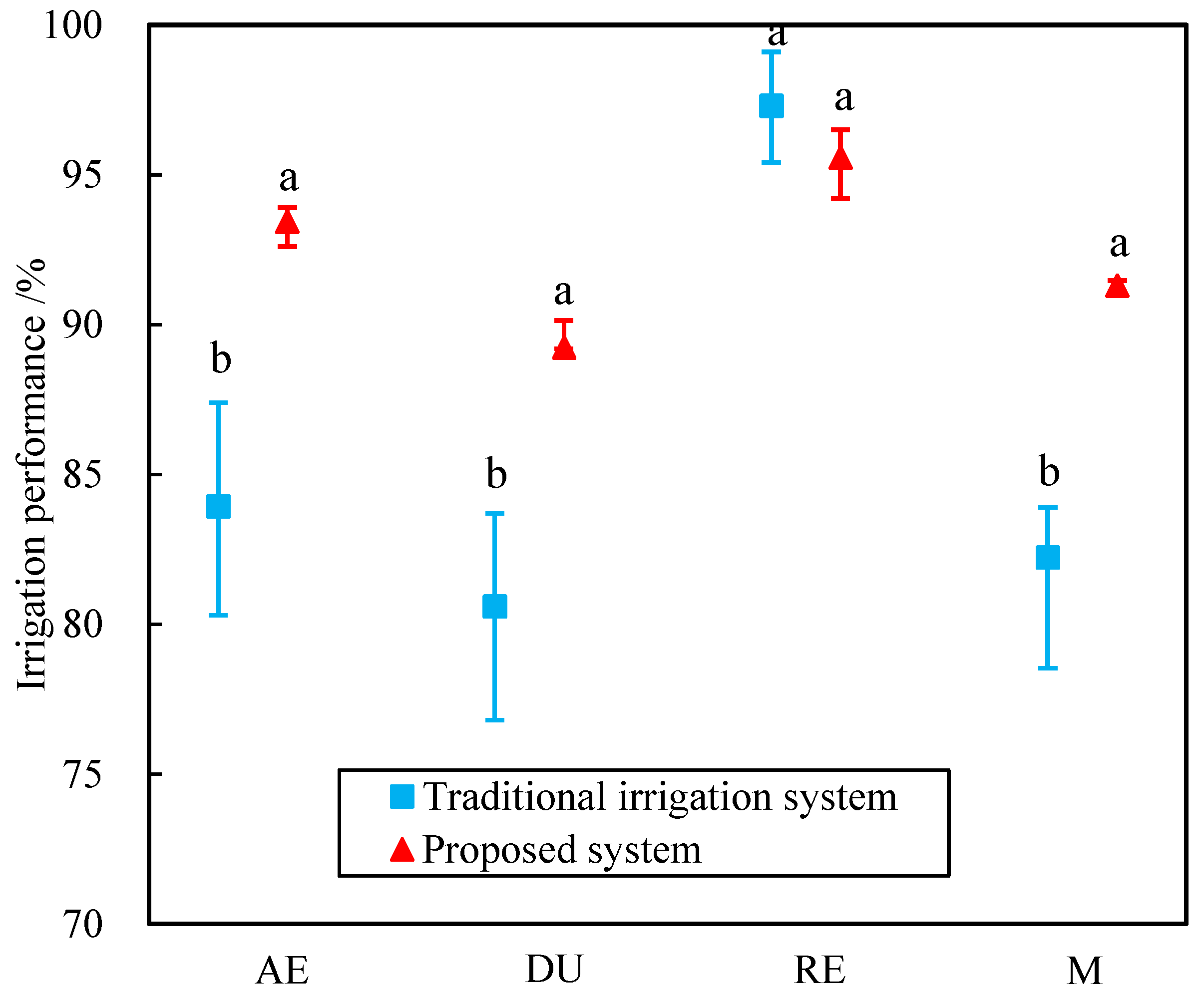
Figure 7 shows the calculation results of the irrigation performance for each field validation experiment. The various irrigation-performance indicators of the proposed system are satisfactory. Except for the DU (range: 88.37–90.13%), the AE, RE, and M for each border all exceed 90%. The averages of the AE, DU, and RE are 93.43%, 89.24%, and 95.57%, respectively. Due to the larger amount of irrigation water, RE for the traditional constant-discharge border irrigation system is equivalent to or even slightly greater than that of the proposed system. The AE, DU, and M for the proposed system are significantly greater than those of the conventional border irrigation system, with average values of 11.3%, 10.7%, and 11.0% greater than the conventional border irrigation system, respectively. This indicates that the proposed system can effectively compensate for the adverse impact of the natural parameter variation on irrigation performance.
Traditional real-time control irrigation systems estimate natural parameters in real time and simulate the irrigation process based on these parameters to determine the optimal irrigation flow rate or stop time, achieving automation and improving the irrigation performance. Khatri et al. [38] simulated their real-time regulation irrigation system, and obtained irrigation performance as follows: AE, DU, and RE of 90.5%, 91.4%, and 93.5%, respectively. Koech et al. [33] measured the average values of the AE, DU, and RE of their proposed real-time regulated irrigation system through field experiments, which were 73.4%, 88.36%, and 98.18%, respectively. The AE, DU, and RE of the real-time regulated furrow irrigation system developed by Khatri and Smith were 82.1%, 90.2%, and 92.5%, respectively [21]. In addition, the real-time adaptive control irrigation system (RACI), which directly adjusts the inflow rate to the system’s maximum or minimum value based on the difference between the actual and expected advance time to avoid calculating natural parameters, achieved 93.0%, 88.4% and 95.4% for the AE, DU and RE, respectively [24]. Overall, the irrigation performance of the proposed system shows slight improvement compared to these automatic border irrigation systems, which have already achieved considerable irrigation efficiency. Due to different control strategies, the proposed system differs from the traditional real-time control irrigation system and the RACI in operational and computational characteristics, as shown in Table 1. As a result of fewer surface flow sensors and simpler computing equipment, the proposed system has more potential for widespread application than the existing automatic border irrigation systems.
4. Conclusions
This study demonstrates the development of an adaptive border irrigation system. During irrigation, the inflow rate is automatically adjusted based only on the deviation of the advance time at the observation points, thereby avoiding the calculation of soil infiltration properties. Therefore, the proposed system greatly simplifies calculations and reduces the requirements of field computing equipment as compared with traditional real-time control irrigation systems. The simulation and experiments show that the proposed system produces a satisfactory irrigation performance. The proposed system has the potential to be widely used in areas lacking irrigation water and agricultural labor.
The proposed system establishes a functional relationship between advance time deviation and optimally adjusted inflow rate as an inflow adjustment strategy. Three sets of border irrigations with significant differences (different locations, crops, natural parameters, irrigation water requirement) showed that advance time deviation and optimally adjusted inflow rate fitted well with the same exponential function, especially during the first inflow adjustment. Moreover, sensitivity analysis and field experiments further validated the achievement of good irrigation performance according to this strategy. The underlying reason for making the strategy effective was the focus of in-depth research. In addition, sensitivity analysis showed that the border length and soil infiltration parameters had a significant impact on the adaptive border irrigation system. Future research should undertake tests on more diverse border fields, especially those with different border lengths and soil infiltrations, to evaluate the advantages of the proposed system for improving irrigation performance.
Author Contributions
Formal analysis, investigation, data curation, writing—original draft: K.L.; formal analysis, visualization, writing—review and editing: X.J.; conceptualization, methodology: W.G.; supervision, writing—review and editing: J.L.; writing—review and editing, visualization: Z.G. All authors have read and agreed to the published version of the manuscript.
Funding
This research was funded by the National Natural Science Foundation of China (Nos. 52309048, 52009030); the Fundamental Research Funds for the Central Universities (No. B220202033); and the Jiangsu Provincial Key Research and Development Program (BE2022390).
Data Availability Statement
Data are contained within the article.
Conflicts of Interest
The authors declare no conflict of interest.
References
- Caner, Y.; Ustun, S.; Selda, O.; Fatih, M.K. Improvement of water and crop productivity of silage maize by irrigation with different levels of recycled wastewater under conventional and zero tillage conditions. Agric. Water Manag. 2023, 277, 108100. [Google Scholar]
- Zhang, F.; Chen, X.; Vitousek, P.M. Chinese agriculture: An experiment for the world. Nature 2013, 497, 33–35. [Google Scholar] [CrossRef] [PubMed]
- Nie, W.B.; Li, Y.B.; Zhang, F.; Ma, X.Y. Optimal discharge for closed-end border irrigation under soil infiltration variability. Agric. Water Manag. 2019, 221, 58–65. [Google Scholar] [CrossRef]
- Xu, J.; Cai, H.; Saddique, Q.; Wang, X.; Li, L.; Ma, C.; Lu, Y. Evaluation and optimization of border irrigation in different irrigation seasons based on temporal variation of infiltration and roughness. Agric. Water Manag. 2019, 214, 64–77. [Google Scholar] [CrossRef]
- Nie, W.B.; Dong, S.X.; Li, Y.B.; Ma, X.Y. Optimization of the border size on the irrigation district scale—Example of the Hetao irrigation district. Agric. Water Manag. 2021, 248, 106768. [Google Scholar] [CrossRef]
- Bai, M.; Li, Y.; Tu, S.; Liu, Q. Analysis on cutoff time optimization of border irrigation to improve irrigated water quality. Trans. Chin. Soc. Agric. Eng. 2016, 32, 105–110. [Google Scholar]
- Chen, B.; Ouyang, Z.; Sun, Z.; Wu, L.; Li, F. Evaluation on the potential of improving border irrigation performance through border dimensions optimization: A case study on the irrigation districts along the lower Yellow River. Irrig. Sci. 2013, 31, 715–728. [Google Scholar] [CrossRef]
- Smith, R.J.; Uddin, M.J. Selection of flow rate and irrigation duration for high performance bay irrigation. Agric. Water Manag. 2020, 228, 11. [Google Scholar] [CrossRef]
- Wu, C.; Bai, M.; Li, Y. Review on intelligent management of surface irrigation under intensive condition. J. Water Resour. Archit. Eng. 2019, 017, 222–227. (In Chinese) [Google Scholar]
- Morris, M.R.; Hussain, A.; Gillies, M.H.; O’Halloran, N.J. Inflow rate and border irrigation performance. Agric. Water Manag. 2015, 155, 76–86. [Google Scholar] [CrossRef]
- Mazarei, R.; Soltani Mohammadi, A.; Ebrahimian, H.; Naseri, A.A. Temporal variability of infiltration and roughness coefficients and furrow irrigation performance under different inflow rates. Agric. Water Manag. 2021, 245, 106465. [Google Scholar] [CrossRef]
- Gonzalez, C.R.; Cervera, L.; Moretfernandez, D. Basin irrigation design with longitudinal slope. Agric. Water Manag. 2011, 98, 1516–1522. [Google Scholar] [CrossRef]
- Smith, R.J.; Uddin, J.M.; Gillies, M.H.; Moller, P.; Clurey, K. Evaluating the performance of automated bay irrigation. Irrig. Sci. 2016, 34, 175–185. [Google Scholar] [CrossRef]
- Abioye, E.A.; Abidin, M.S.Z.; Mahmud, M.S.A.; Buyamin, S.; Ishak, M.H.I.; Abd Rahman, M.K.I.; Otuoze, A.O.; Onotu, P.; Ramli, M.S.A. A review on monitoring and advanced control strategies for precision irrigation. Comput. Electron. Agric. 2020, 173, 22. [Google Scholar] [CrossRef]
- Zhao, H.; Di, L.; Yu, E.; Guo, L.; Li, L.; Zhang, C.; Li, L. A Review of Scientific Irrigation Scheduling Methods. In Proceedings of the 2023, 11th International Conference on Agro-Geoinformatics (Agro-Geoinformatics), Wuhan, China, 25–28 July 2023; pp. 1–4. [Google Scholar] [CrossRef]
- Zhao, H.; Di, L.; Guo, L.; Zhang, C.; Lin, L. An Automated Data-Driven Irrigation Scheduling Approach Using Model Simulated Soil Moisture and Evapotranspiration. Sustainability 2023, 15, 12908. [Google Scholar] [CrossRef]
- Zhao, H.; Di, L.; Guo, L.; Zhang, C.; Yu, E.; Li, H. Optimizing Irrigation Scheduling Using Deep Reinforcement Learning. In Proceedings of the 2023, 11th International Conference on Agro-Geoinformatics (Agro-Geoinformatics), Wuhan, China, 25–28 July 2023; pp. 1–4. [Google Scholar] [CrossRef]
- Reddell, D.; Latimer, E. Advance Rate Feedback Irrigation System (ARFIS); Microfiche Collection (USA); American Society of Agricultural Engineers: St. Joseph, MI, USA, 1986. [Google Scholar]
- Latimer, E.; Reddell, D. Components for an advance rate feedback irrigation system (ARHS). Trans. ASAE 1990, 33, 1162–1170. [Google Scholar] [CrossRef]
- Clemmens, A.; Keats, J. Bayesian inference for feedback control. II: Surface irrigation example. J. Irrig. Drain. Eng. 1992, 118, 416–432. [Google Scholar] [CrossRef]
- Khatri, K.L.; Smith, R. Toward a simple real-time control system for efficient management of furrow irrigation. Irrig. Drain. J. Int. Comm. Irrig. Drain. 2007, 56, 463–475. [Google Scholar] [CrossRef]
- Koech, R.; Smith, R.; Gillies, M. A real-time optimisation system for automation of furrow irrigation. Irrig. Sci. 2014, 32, 319–327. [Google Scholar] [CrossRef]
- Li, J.; Huang, Z.; Li, T.; Jiao, X.; Shi, C. Regulation of border irrigation technical elements considering condition of uneven initial soil moisture content along border. Trans. Chin. Soc. Agric. Mach. 2023, 54, 320–329+370. (In Chinese) [Google Scholar]
- Liu, K.; Jiao, X.; Jiang, L.; Gu, Z.; Guo, W. A Real-Time Adaptive Control System for Border Irrigation. Agronomy 2022, 12, 2995. [Google Scholar] [CrossRef]
- Salahou, M.K.; Jiao, X.; Lü, H. Border irrigation performance with distance-based cut-off. Agric. Water Manag. 2018, 201, 27–37. [Google Scholar] [CrossRef]
- Wu, C.; Xu, D.; Bai, M.; Li, Y.; Li, F. Real-time feedback control technology for precise furrow irrigation. J. Drain. Irrig. Mach. Eng. 2020, 38, 536–540. (In Chinses) [Google Scholar]
- Jiao, X.; Wang, W. Robust Design of Border Irrigation and Furrow Irrigation; Hohai University Press: Nanjing, China, 2012. (In Chinese) [Google Scholar]
- Bautista, E.; Clemmens, A.J.; Strelkoff, T.S.; Schlegel, J. Modern analysis of surface irrigation systems with WinSRFR. Agric. Water Manag. 2009, 96, 1146–1154. [Google Scholar] [CrossRef]
- Liu, K.; Jiao, X.; Li, J.; An, Y.; Guo, W.; Salahou, M.K.; Sang, H. Performance of a zero-inertia model for irrigation with rapidly varied inflow discharges. Int. J. Agric. Biol. Eng. 2020, 13, 175–181. [Google Scholar] [CrossRef]
- Schwankl, L.; Raghuwanshi, N.; Wallender, W. Furrow irrigation performance under spatially varying conditions. J. Irrig. Drain. Eng. 2000, 126, 355–361. [Google Scholar] [CrossRef]
- Trout, T.J.; Mackey, B.E. Furrow inflow and infiltration variability. Trans. ASAE 1988, 31, 531–0537. [Google Scholar] [CrossRef]
- Nie, W.-B.; Li, Y.-B.; Zhang, F.; Dong, S.-X.; Wang, H.; Ma, X.-Y. A Method for Determining the Discharge of Closed-End Furrow Irrigation Based on the Representative Value of Manning’s Roughness and Field Mean Infiltration Parameters Estimated Using the PTF at Regional Scale. Water 2018, 10, 1825. [Google Scholar] [CrossRef]
- Koech, R.K.; Smith, R.J.; Gillies, M.H. Evaluating the performance of a real-time optimisation system for furrow irrigation. Agric. Water Manag. 2014, 142, 77–87. [Google Scholar] [CrossRef]
- Lei, G.; Fan, G. Practical Optimization Model for Technical Parameters of Border Irrigation. Yellow River 2017, 39, 149–152. (In Chinese) [Google Scholar]
- Bautista, E.; Wallender, W. Spatial variability of infiltration in furrows. Trans. ASAE 1985, 28, 1846–1851. [Google Scholar] [CrossRef]
- Nie, W.; Fei, L.; Ma, X. Effects of Spatial Variability of Soil Infiltration Characteristics and Manning Roughness on Furrow Irrigation Performance. Trans. Chin. Soc. Agric. Mach. 2014, 45, 108–114. (In Chinese) [Google Scholar]
- Liu, K.H.; Jiao, X.Y.; Guo, W.H.; An, Y.H.; Salahou, M.K. Improving border irrigation performance with predesigned varied-discharge. PLoS ONE 2020, 15, e232751. [Google Scholar] [CrossRef] [PubMed]
- Khatri, K.L.; Memon, A.A.; Shaikh, Y.; Pathan, A.; Shah, S.A.; Pinjani, K.K.; Soomro, R.; Smith, R.; Almani, Z. Real-Time Modelling and Optimisation for Water and Energy Efficient Surface Irrigation. J. Water Resour. Prot. 2013, 5, 681–688. [Google Scholar] [CrossRef]
Figure 1.
Flowchart of the adaptive border irrigation process. Qc is the actual inflow rate (L s−1); QMIN is the minimum inflow rate set in the border irrigation system (L s−1); QMAX is the maximum inflow rate set in the border irrigation system (L s−1); VA is the volume of accumulated irrigation (m3); tA is the actual water inflow advance time (s); tE is the expected water inflow advance time (s).

Figure 2.
Components of the proposed system.

Figure 3.
First inflow adjustment strategy.

Figure 4.
Second inflow adjustment strategy.
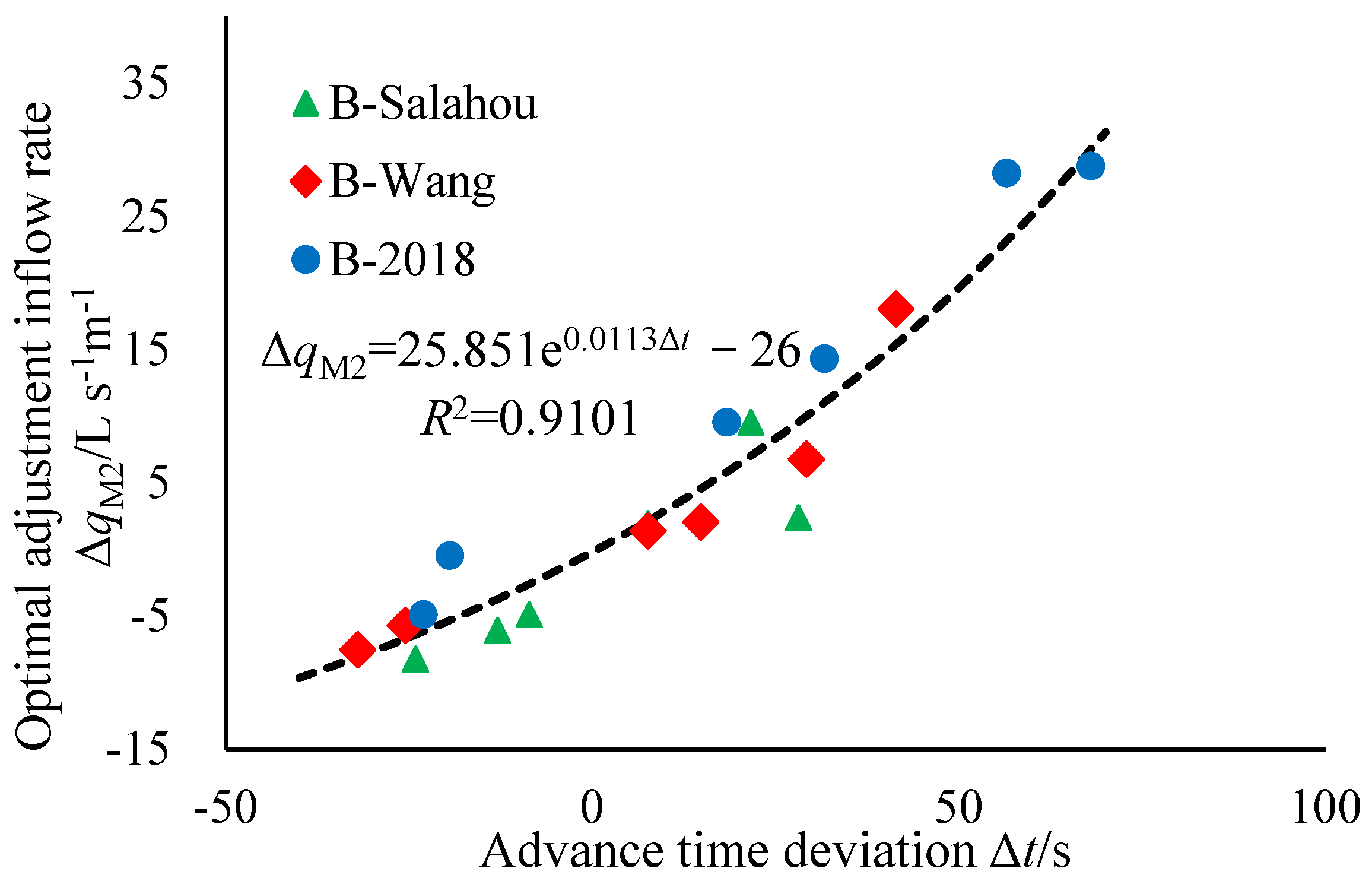
Figure 5.
Irrigation performance of the proposed system when the natural parameters are varied by (a) ±10% and (b) ±20%. The columns indicate the irrigation performance without the natural parameter variation, and the vertical bars indicate the standard deviations of the irrigation performance under the natural parameter variation.
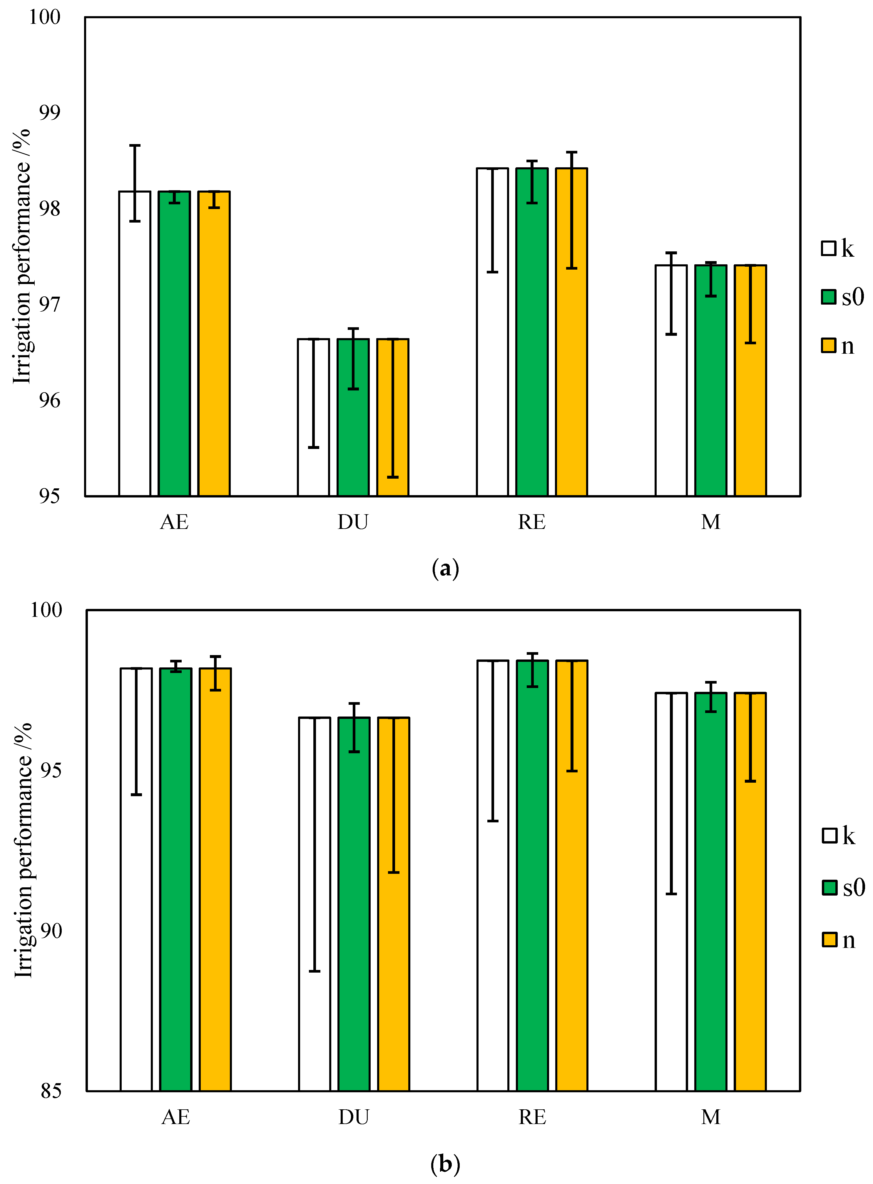
Figure 6.
Irrigation performance of the proposed system considering the inflow rate control error. The columns indicate the irrigation performance without the inflow rate control error, and the vertical bars indicate the standard deviations of the irrigation performance under the inflow rate control error.
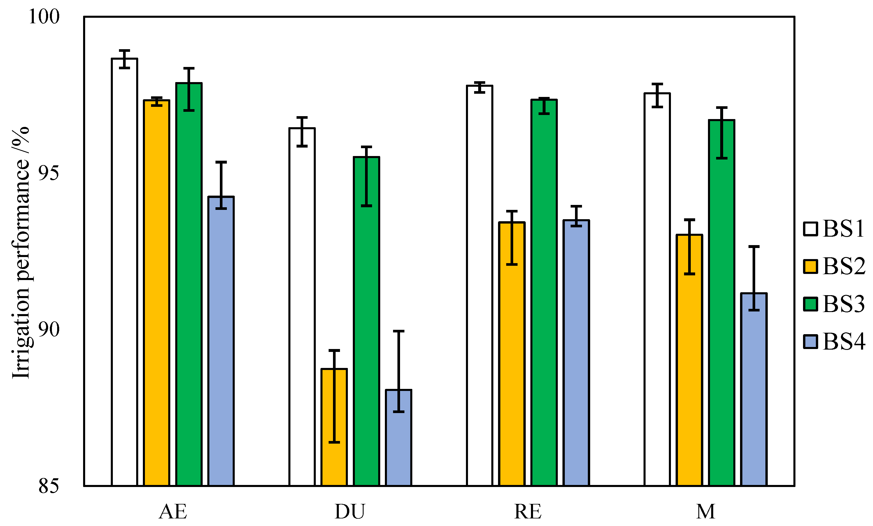
Figure 7.
Irrigation performance of the proposed system compared with that of the traditional constant-discharge border irrigation system. The vertical bars labeled with “a” and “b” for each irrigation-performance indicator indicate significant differences at p = 0.05, based on the independent sample t-test.

Table 1.
Comparisons between the proposed system, the RACI, and the traditional real-time control irrigation system.
Table 1.
Comparisons between the proposed system, the RACI, and the traditional real-time control irrigation system.
| Comparison | Proposed System | RACI | Traditional Real-Time Control Irrigation | ||
|---|---|---|---|---|---|
| Surface flow sensors | Layout | The first monitoring point is located at 40 m, and the spacing between subsequent monitoring points is 30 m | The first monitoring point is located at 40 m, and the spacing between subsequent monitoring points is 10 m | The monitoring points are concentrated in the front section of the border field (usually no less than 60 m), and the layout interval is usually 5 m or 10 m | |
| Amount for a classic border | 100-m-long border | 2 | 5 | 5 or 12 | |
| 150-m-long border | 4 | 10 | 5 or 12 | ||
| 200-m-long border | 5 | 13 | 5 or 12 | ||
| Adjustment basis | Difference between actual and expected advance time and inflow adjustment strategy | Difference between actual and expected advance time | Real-time calculation of natural parameters and simulation of irrigation process | ||
| Calculation | Function | Exponential function | Logic function | Partial differential equations | |
| Equipment requirements | Simple computing equipment (such as single-chip microcomputer) | Simple computing equipment (such as single-chip microcomputer) | Equipment capable of performing complex calculations in a short time (such as computer) | ||
Table 2.
Natural parameters of each border.
| Border | Border Specification | Infiltration Parameters | Slope s0 | Roughness n | Irrigation Water Requirement m (mm) | ||
|---|---|---|---|---|---|---|---|
| Length L (m) | Width D (m) | k (mm min−α) | α | ||||
| B-Salahou | 100 | 3.7 | 7.55 | 0.68 | 0.0025 | 0.06 | 60 |
| B-2018 | 100 | 3.0 | 13.94 | 0.47 | 0.0017 | 0.16 | 90 |
| B-Wang | 110 | 2.0 | 9.30 | 0.58 | 0.0034 | 0.08 | 60 |
Table 3.
Natural parameters of the simulated scenarios.
| Number | Simulated Scenarios | Natural Parameters | |||
|---|---|---|---|---|---|
| Infiltration Parameters | Slope s0 | Roughness n | |||
| K (mm min−α) | α | ||||
| BS0 | Original value | 13.94 | 0.47 | 0.0017 | 0.16 |
| BS1 | Infiltration coefficient +10% | 15.33 | 0.47 | 0.0017 | 0.16 |
| BS2 | Infiltration coefficient +20% | 16.44 | 0.47 | 0.0017 | 0.16 |
| BS3 | Infiltration coefficient −10% | 12.55 | 0.47 | 0.0017 | 0.16 |
| BS4 | Infiltration coefficient −20% | 11.15 | 0.47 | 0.0017 | 0.16 |
| BS5 | Slope +10% | 13.94 | 0.47 | 0.0019 | 0.16 |
| BS6 | Slope +20% | 13.94 | 0.47 | 0.0020 | 0.16 |
| BS7 | Slope −10% | 13.94 | 0.47 | 0.0015 | 0.16 |
| BS8 | Slope −20% | 13.94 | 0.47 | 0.0014 | 0.16 |
| BS9 | Roughness +10% | 13.94 | 0.47 | 0.0017 | 0.17 |
| BS10 | Roughness +20% | 13.94 | 0.47 | 0.0017 | 0.19 |
| BS11 | Roughness −10% | 13.94 | 0.47 | 0.0017 | 0.15 |
| BS12 | Roughness −20% | 13.94 | 0.47 | 0.0017 | 0.13 |
Table 4.
Optimal constant-discharge irrigation scheme of B-Salahou, B-2018, and B-Wang.
| Border | Optimal Constant-Discharge Irrigation Scheme | Expected Advance Time of Observation Points (min) | Irrigation Performance (%) | ||||
|---|---|---|---|---|---|---|---|
| Inflow Rate q0 (L s−1 m−1) | Cut-Off Time tT (min) | 40 m | 70 m | AE | DU | RE | |
| B-Salahou | 6.2 | 16.13 | 6.24 | 13.00 | 97.87 | 92.60 | 95.23 |
| B-2018 | 4.8 | 31.26 | 14.03 | 29.01 | 98.19 | 96.64 | 97.41 |
| B-Wang | 5.8 | 18.97 | 7.75 | 15.22 | 96.12 | 93.34 | 94.73 |
Table 5.
Optimal inflow adjustment scheme at 40 m.
| Border | Infiltration Parameters k (mm min−α) | Initial Flow Rate q0 (L s−1 m−1) | Advance Time Deviation Δt (s) | Optimal Adjustment Inflow Rate ΔqM1 (L s−1 m−1) | Inflow Rate after Adjustment qM1 (L s−1 m−1) | Irrigation Performance M (%) |
|---|---|---|---|---|---|---|
| B-Salahou | 8.17 | 6.2 | 7.9 | 1.1 | 7.3 | 93.83 |
| 8.79 | 6.2 | 17.6 | 3.3 | 9.5 | 93.29 | |
| 7.55 | 6.2 | 0 | 0 | 6.2 | 94.36 | |
| 6.93 | 6.2 | −9.4 | −1.4 | 4.8 | 95.32 | |
| 6.32 | 6.2 | −46.4 | −2.3 | 3.9 | 95.46 | |
| 9.41 | 6.2 | 27.7 | 5.7 | 11.9 | 93.06 | |
| B-2018 | 15.97 | 4.8 | 33.1 | 7.2 | 12.0 | 97.86 |
| 13.69 | 4.8 | −18.7 | −1.4 | 3.4 | 97.32 | |
| 14.14 | 4.8 | −8.6 | −0.9 | 3.9 | 97.23 | |
| 15.21 | 4.8 | 15.5 | 1.9 | 6.7 | 97.42 | |
| 16.42 | 4.8 | 43.9 | 12.7 | 17.5 | 97.66 | |
| 12.93 | 4.8 | −35.3 | −2.2 | 2.6 | 97.47 | |
| B-Wang | 10.23 | 5.8 | 14.8 | 1.7 | 7.5 | 93.95 |
| 10.89 | 5.8 | 25.6 | 3.7 | 9.5 | 94.20 | |
| 8.56 | 5.8 | −11.2 | −1.5 | 4.3 | 94.31 | |
| 7.91 | 5.8 | −20.2 | −2.3 | 3.5 | 94.83 | |
| 11.35 | 5.8 | 33.5 | 6.9 | 12.7 | 94.38 | |
| 7.44 | 5.8 | −26.6 | −2.6 | 3.2 | 94.72 |
Table 6.
Optimal inflow adjustment scheme at 40 m and 70 m.
| Border | Initial Flow Rate q0 (L s−1 m−1) | First Adjustment (40 m) | Second Adjustment (70 m) | Irrigation Performance M (%) | ||||
|---|---|---|---|---|---|---|---|---|
| Advance Time Deviation Δt1 (s) | Optimal Adjustment Inflow Rate ΔqM1 (L s−1 m−1) | Inflow Rate after Adjustment qM1 (L s−1 m−1) | Advance Time Deviation Δt2 (s) | Optimal Adjustment Inflow Rate ΔqM2 (L s−1 m−1) | Inflow Rate after Adjustment qM2 (L s−1 m−1) | |||
| B-Salahou | 6.2 | −6.5 | 1.9 | 8.1 | −13.0 | −6.1 | 2.0 | 92.45 |
| 6.2 | 6.5 | −1.1 | 5.1 | 7.6 | 1.9 | 7.0 | 94.60 | |
| 6.2 | −11.8 | 2.2 | 8.4 | −8.6 | −4.9 | 3.5 | 94.24 | |
| 6.2 | 4.68 | −0.8 | 5.4 | 28.1 | 2.4 | 7.8 | 93.35 | |
| 6.2 | −3.96 | −0.7 | 5.5 | 21.6 | 9.6 | 15.1 | 94.05 | |
| 6.2 | −7.56 | 3 | 9.2 | −24.1 | −8.2 | 1.0 | 91.56 | |
| B-2018 | 4.8 | 15.5 | −0.8 | 4.0 | 18.4 | 9.5 | 13.5 | 97.07 |
| 4.8 | −9.4 | 0.6 | 5.4 | −23.0 | −4.9 | 0.5 | 96.13 | |
| 4.8 | 17.3 | −1.3 | 3.5 | 68.0 | 28.8 | 32.3 | 97.38 | |
| 4.8 | −5.0 | 0.4 | 5.2 | −19.4 | −0.5 | 4.7 | 95.87 | |
| 4.8 | −4.3 | −0.6 | 4.2 | 31.9 | 14.3 | 18.5 | 96.17 | |
| 4.8 | 21.2 | −0.9 | 3.9 | 56.5 | 28.2 | 32.1 | 97.03 | |
| B-Wang | 5.8 | 19.4 | 2.7 | 8.5 | −32.0 | −7.5 | 1.0 | 92.44 |
| 5.8 | 16.6 | 2.1 | 7.9 | −25.6 | −5.7 | 2.2 | 94.48 | |
| 5.8 | −18.4 | −1.7 | 4.1 | 7.6 | 1.4 | 5.5 | 94.32 | |
| 5.8 | −13.7 | −1.4 | 4.4 | 14.8 | 2 | 6.4 | 94.72 | |
| 5.8 | −31.7 | −2.3 | 3.5 | 29.2 | 6.8 | 10.3 | 91.02 | |
| 5.8 | −47.9 | −2.7 | 3.1 | 41.4 | 18 | 21.1 | 92.33 | |
Table 7.
The adaptive border irrigation scheme under the scenario of the natural parameter changes.
| Border | Simulated Scenarios | Initial Flow Rate q0 (L s−1 m−1) | First Adjustment (40 m) | Second Adjustment (70 m) | Cut-Off Time tT (min) | ||
|---|---|---|---|---|---|---|---|
| Advance Time t40 (min) | Inflow Rate after Adjustment q1 (L s−1 m−1) | Advance Time t70 (min) | Inflow Rate after Adjustment q2 (L s−1 m−1) | ||||
| BS0 | Original value | 4.8 | 14.03 | —— | 29.01 | —— | 31.26 |
| BS1 | Infiltration coefficient +10% | 4.8 | 14.52 | 10.30 | —— | 22.32 | |
| BS2 | Infiltration coefficient +20% | 4.8 | 14.88 | 20.00 | —— | 18.81 | |
| BS3 | Infiltration coefficient −10% | 4.8 | 13.49 | 2.50 | 32.21 | 20.00 | 34.13 |
| BS4 | Infiltration coefficient −20% | 4.8 | 12.90 | 1.80 | 31.80 | 20.00 | 34.50 |
| BS5 | Slope +10% | 4.8 | 13.09 | 3.90 | 29.70 | 19.20 | 30.83 |
| BS6 | Slope +20% | 4.8 | 13.81 | 3.40 | 30.80 | 20.00 | 32.07 |
| BS7 | Slope −10% | 4.8 | 14.10 | 5.10 | 28.93 | 3.60 | 30.73 |
| BS8 | Slope −20% | 4.8 | 14.26 | 6.60 | —— | 26.64 | |
| BS9 | Roughness +10% | 4.8 | 14.16 | 5.60 | 28.74 | 1.10 | 29.07 |
| BS10 | Roughness +20% | 4.8 | 15.06 | 20.00 | —— | 18.95 | |
| BS11 | Roughness −10% | 4.8 | 13.80 | 3.40 | 30.78 | 20.00 | 32.08 |
| BS12 | Roughness −20% | 4.8 | 13.38 | 2.30 | 32.76 | 20.00 | 34.82 |
Note: ‘——’ indicates that the surface flow has not advanced to this point, but has been stopped due to the irrigation volume reaching the amount of required irrigation water, so there is no inflow rate adjustment conducted here.
Table 8.
The adaptive border irrigation scheme under the scenario of inflow rate control errors.
| Border | Simulated Scenarios | Initial Flow Rate q0 (L s−1 m−1) | First Adjustment (40 m) | Second Adjustment (70 m) | Cut-Off Time tT (min) | ||
|---|---|---|---|---|---|---|---|
| Advance Time t40 (min) | Inflow Rate after Adjustment q1 (L·s−1·m−1) | Advance Time t70 (min) | Inflow Rate after Adjustment q2 (L s−1 m−1) | ||||
| BS1 | No control error in inflow rate | 4.8 | 14.52 | 10.30 | —— | 22.32 | |
| +10% control error in inflow rate | 4.8 | 14.52 | 11.30 | —— | 21.62 | ||
| −10% control error in inflow rate | 4.8 | 14.52 | 9.30 | —— | 23.20 | ||
| BS2 | No control error in inflow rate | 4.8 | 14.88 | 20.00 | —— | 18.81 | |
| +10% control error in inflow rate | 4.8 | 14.88 | 22.00 | —— | 19.25 | ||
| −10% control error in inflow rate | 4.8 | 14.88 | 18.00 | —— | 18.45 | ||
| BS3 | No control error in inflow rate | 4.8 | 13.49 | 2.50 | 32.21 | 20.00 | 34.13 |
| +10% control error in inflow rate | 4.8 | 13.49 | 2.80 | 31.14 | 22.00 | 32.70 | |
| −10% control error in inflow rate | 4.8 | 13.49 | 2.30 | 29.70 | 18.00 | 35.03 | |
| BS4 | No control error in inflow rate | 4.8 | 12.90 | 1.80 | 31.80 | 20.00 | 34.50 |
| +10% control error in inflow rate | 4.8 | 12.90 | 2.00 | 31.50 | 22.00 | 33.83 | |
| −10% control error in inflow rate | 4.8 | 12.90 | 1.60 | 32.82 | 18.00 | 35.92 | |
Note: ‘——’ indicates that the surface flow has not advanced to this point, but has been stopped due to the irrigation volume reaching the amount of required irrigation water, so there is no inflow rate adjustment conducted here.
Table 9.
The adaptive border irrigation scheme under the scenario of border length changes.
| Border Length L (m) | Simulated Scenarios | Initial Flow Rate q0 (L s−1 m−1) | First Adjustment (40 m) | Second Adjustment (70 m) | First Adjustment (100 m) | Second Adjustment (130 m) | Second Adjustment (160 m) | Cut-Off Time tT (min) | |||||
|---|---|---|---|---|---|---|---|---|---|---|---|---|---|
| Advance Time t40 (min) | Inflow Rate after Adjustment q1 (L s−1 m−1) | Advance Time t70 (min) | Inflow Rate after Adjustment q2 (L s−1 m−1) | Advance Time t40 (min) | Inflow Rate after Adjustment q1 (L s−1 m−1) | Advance Time t70 (min) | Inflow Rate after Adjustment q2 (L s−1 m−1) | Advance Time t70 (min) | Inflow Rate after Adjustment q2 (L s−1 m−1) | ||||
| 150 | BS0 | 4.8 | 10.68 | —— | 21.30 | —— | 34.09 | —— | —— | —— | 34.10 | ||
| BS1 | 4.8 | 10.86 | 7.80 | 21.45 | 10.50 | —— | —— | —— | 28.18 | ||||
| BS2 | 4.8 | 11.04 | 9.90 | 21.20 | 8.10 | —— | —— | —— | 27.55 | ||||
| BS3 | 4.8 | 10.32 | 4.70 | 21.37 | 5.80 | 35.90 | 20.00 | —— | —— | 36.92 | |||
| BS4 | 4.8 | 9.88 | 3.90 | 21.18 | 1.70 | 39.20 | 20.00 | —— | —— | 43.48 | |||
| 200 | BS0 | 4.8 | 8.47 | —— | 16.61 | —— | 25.54 | —— | —— | —— | 34.88 | ||
| BS1 | 4.8 | 8.70 | 10.30 | 16.71 | 12.00 | 25.20 | 6.50 | —— | —— | 31.38 | |||
| BS2 | 4.8 | 8.82 | 11.80 | 16.68 | 12.90 | 24.78 | 2.30 | 32.22 | 1.00 | 41.26 | 1.00 | 41.76 | |
| BS3 | 4.8 | 8.26 | 7.30 | 16.31 | 2.50 | 25.92 | 9.90 | —— | —— | 40.77 | |||
| BS4 | 4.8 | 8.05 | 6.60 | 15.89 | 1.00 | 25.76 | 5.10 | 44.70 | 20.00 | —— | 48.38 | ||
Note: BS0 was the constant-discharge irrigation without inflow rate adjustment. ‘——’ for other simulated scenario indicates that the surface flow has not advanced to this point, but has been stopped due to the irrigation volume reaching the amount of required irrigation water, so there is no inflow rate adjustment conducted here.
Table 10.
Irrigation performance of the proposed system under border length changes.
| Border Length | Simulated Scenarios | Irrigation Performance (%) | |||
|---|---|---|---|---|---|
| AE | DU | RE | M | ||
| 150 m | BS1 | 96.29 | 91.00 | 93.57 | 93.61 |
| BS2 | 92.92 | 89.93 | 93.43 | 91.41 | |
| BS3 | 95.24 | 91.98 | 96.36 | 93.60 | |
| BS4 | 93.84 | 89.53 | 93.89 | 91.66 | |
| 200 m | BS1 | 96.11 | 92.85 | 99.81 | 94.47 |
| BS2 | 91.32 | 84.07 | 99.93 | 87.62 | |
| BS3 | 93.58 | 88.95 | 95.48 | 91.24 | |
| BS4 | 91.56 | 85.63 | 92.07 | 88.55 | |
Disclaimer/Publisher’s Note: The statements, opinions and data contained in all publications are solely those of the individual author(s) and contributor(s) and not of MDPI and/or the editor(s). MDPI and/or the editor(s) disclaim responsibility for any injury to people or property resulting from any ideas, methods, instructions or products referred to in the content. |
© 2023 by the authors. Licensee MDPI, Basel, Switzerland. This article is an open access article distributed under the terms and conditions of the Creative Commons Attribution (CC BY) license (https://creativecommons.org/licenses/by/4.0/).
Share and Cite
MDPI and ACS Style
Liu, K.; Jiao, X.; Guo, W.; Gu, Z.; Li, J. Improving Irrigation Performance by Using Adaptive Border Irrigation System. Agronomy 2023, 13, 2907. https://doi.org/10.3390/agronomy13122907
AMA Style
Liu K, Jiao X, Guo W, Gu Z, Li J. Improving Irrigation Performance by Using Adaptive Border Irrigation System. Agronomy. 2023; 13(12):2907. https://doi.org/10.3390/agronomy13122907
Chicago/Turabian StyleLiu, Kaihua, Xiyun Jiao, Weihua Guo, Zhe Gu, and Jiang Li. 2023. "Improving Irrigation Performance by Using Adaptive Border Irrigation System" Agronomy 13, no. 12: 2907. https://doi.org/10.3390/agronomy13122907
Note that from the first issue of 2016, this journal uses article numbers instead of page numbers. See further details here.