Article

Estimating the Light Interception and Photosynthesis of Greenhouse-Cultivated Tomato Crops under Different Canopy Configurations

1
College of Agronomy and Life Science, Shanxi Datong University, Datong 037009, China
2
College of Horticulture, Shenyang Agricultural University, No. 120 Dongling Road, Shenyang 110866, China
3
College of Agronomy, Hunan Agricultural University, Changsha 410128, China
4
Key Laboratory of Protected Horticulture, Ministry of Education, Shenyang 110866, China
5
National & Local Joint Engineering Research Center of Northern Horticultural Facilities Design & Application Technology (Liaoning), No. 120 Dongling Road, Shenyang 110866, China
6
College of Engineering, Shenyang Agricultural University, No. 120 Dongling Road, Shenyang 110866, China
7
Engineering Research Center of Coal-Based Ecological Carbon Sequestration Technology of the Ministry of Education, Shanxi Datong University, Datong 037009, China
8
Key Laboratory of Graphene Forestry Application of National Forest and Grass Administration, Shanxi Datong University, Datong 037009, China
*
Authors to whom correspondence should be addressed.
Agronomy 2024, 14(2), 249; https://doi.org/10.3390/agronomy14020249
Submission received: 27 December 2023 / Revised: 21 January 2024 / Accepted: 22 January 2024 / Published: 24 January 2024
(This article belongs to the Topic Advances in Crop Simulation Modelling)

Abstract

:
Understanding the spatial heterogeneity of light and photosynthesis distribution within a canopy is crucial for optimizing plant growth and yield, especially in the context of greenhouse structures. In previous studies, we developed a 3D functional-structural plant model (FSPM) of the Chinese solar greenhouse (CSG) and tomato plants, in which the greenhouse was reconstructed as a 3D mockup and implemented in the virtual scene. This model, which accounts for various environmental factors, allows for precise calculations of radiation, temperature, and photosynthesis at the organ level. This study focuses on elucidating optimal canopy configurations for mechanized planting in greenhouses, building upon the commonly used north–south (N–S) orientation by exploring the east–west (E–W) orientation. Investigating sixteen scenarios with varying furrow distance (1 m, 1.2 m, 1.4 m, 1.6 m) and row spacing (0.3 m, 0.4 m, 0.5 m, 0.6 m), corresponding to 16 treatments of plant spacing, four planting patterns (homogeneous row, double row, staggered row, incremental row) and two orientations were investigated. The results show that in Shenyang city, an E–W orientation with the path width = 0.5 (furrow distance + row distance) = 0.8 m (homogeneous row), and a plant distance of 0.32 m, is the optimal solution for mechanized planting at a density of 39,000 plants/ha. Our findings reveal a nuanced understanding of how altering planting configurations impacts the light environment and photosynthesis rate within solar greenhouses. Looking forward, these insights not only contribute to the field of CSG mechanized planting, but also provide a basis for enhanced CSG planting management. Future research could further explore the broader implications of these optimized configurations in diverse geographic and climatic conditions.

1. Introduction

Cultivating tomatoes in solar greenhouses is a significant method of tomato production in northern China. This approach not only enables a consistent year-round tomato supply, but also contributes to increased income for farmers, in contrast to traditional field cultivation methods [1]. At present, the N–S ridge is mostly used for tomato cultivation in solar greenhouses in northern China, due to its high space utilization rate and light uniformity [2]. The ridges are short and numerous, which are not suitable for mechanical land preparation (such as ditching, ridging, and seeding) but only manual preparation. With China’s aging population, the ongoing use of north–south ridge greenhouse cultivation is expected to lead to an escalation in labor costs [3]. This has become the main reason for restricting the development of tomato production in solar greenhouses. In order to solve this problem, in recent years, some scholars and producers have changed the N–S ridge cultivation of tomatoes in the Chinese solar greenhouse (CSG) to the E–W row orientation [4]. Many mechanized devices suitable for east–west ridge cultivation in solar greenhouses have been gradually developed, such as ridge forming and mulching machines, transplanting machines, and harvesting and transporting carts. By increasing the ridge length and reducing the number of ridges, the level of mechanized operation was improved, and the degree of simplified cultivation was significantly improved [5]. While east–west ridge cultivation of tomatoes in solar greenhouses is conducive to mechanization, production observations reveal that, in comparison to the prevalent north–south orientation configuration, this approach leads to uneven light distribution and reduced photosynthetic efficiency within the tomato canopy. This issue is particularly pronounced in the north-facing rows, resulting in uneven growth of tomato plants and diminished fruit yield [6]. In order to optimize the light efficiency of the tomato canopy on the east–west ridges of the CSG, the researchers adjusted the cultivation density and canopy configuration and achieved certain results [7]. However, the dynamic dependence between tomato plant density, canopy configuration, optimal light, and photosynthesis distribution has not been confirmed, and the optimal light efficiency of tomato populations on the east–west ridge has not yet been analyzed. As a result, the question of “optimal tomato canopy configuration for east-west ridge cultivation” still remains unresolved.
The light environment inside a solar greenhouse is spatially heterogeneous, and the incident light reaching the canopy through the front cover is not uniformly distributed (Figure 1). Determining how to improve the light environment of the canopy, and thereby the photosynthetic efficiency of the canopy, is crucial. Several studies have indicated that, despite a more noticeable upward trend in light interception, photosynthesis in the upper canopy leaves was more inhibited compared to in the lower canopy leaves [8]. Therefore, an increase in light interception does not in itself imply an increase in photosynthesis and growth; this would only occur if the local photosynthetic capacity is able to use all the absorbed light accordingly. It was found that the net photosynthetic rate of leaves in the greenhouse canopy was significantly correlated with plant spacing [9], furrow distance [10], plant height, and photosynthetic active radiation [11]. Canopy leaf temperature and age are also important factors affecting the photosynthetic rate [12]. Therefore, it is important to consider the temporal and spatial variation of photosynthesis in terms of physical, physiological, and biochemical processes to optimize the canopy photosynthetic capacity in greenhouses [13]. In simpler terms, optimizing the distribution pattern of photosynthetic rates can offer valuable insights for effective cultivation management and improvements in planting configuration. This, in turn, helps in achieving the ultimate goal of maximizing the utilization of light energy in accordance with the specific growth requirements of crops [14].
For studies on the light environment of east–west orientation tomato cultivation, researchers have mostly focused on multi-span glass greenhouses. Some studies have found that the canopy light interception of glass greenhouses in north–south orientation is better than that of east–west orientation [15], but changes in row orientation have limited effect on the photosynthesis of greenhouse crops due to the full light transmittance of glass multi-span greenhouses. During the fall and winter seasons, inconsistent changes in tomato fruit color, uneven fruit size, and large yield fluctuations on the south and north sides of the greenhouse have occurred. The main cause of this phenomenon is that the most commonly used east–west tomato configuration is used in the autumn and winter seasons with a relatively low solar altitude angle, resulting in aggravated shading of the tomato plant canopy on the north side of the canopy row [15] and reduced photosynthetic rate uniformity in the tomato canopy. However, changing the row orientation has a relatively small impact on the light environment of the tomato canopy in spring and summer. In recent years, extensive research has been conducted on greenhouse plant configuration parameters. Findings indicate that the leaves reached light saturation at ridge distances of 1.2 m and 1.6 m [10]. When comparing the distribution of radiation and photosynthesis between planting strategy and plant architecture, altering the planting strategy, such as adjusting plant spacing, has a more pronounced impact on canopy photosynthesis than changes in plant architecture [16]. Based on the above research, canopy configuration can strongly affect the light environment of the tomato canopy, but the dynamic dependence among tomato canopy configuration, optimal light distribution, and photosynthetic efficiency has not been elucidated, and analysis of the canopy configuration of the tomato in the east–west orientation under CSG conditions has not been undertaken.
Compared to the simulation approach, determining the light distribution and photosynthetic efficiency of the tomato canopy in cultivation experiments is more direct and effective, but can be time and labor intensive [17]. Early light environment simulation studies mainly calculated the light interception rate of the canopy based on the leaf area index (LAI) and extinction coefficient [18], and the extinction coefficient was calculated by fitting experimental data with the Lambert–Beer law, or according to specific leaf inclination angle [19]. These methods can be used to roughly estimate the total light interception in the canopy, but cannot capture the effect of canopy heterogeneity on light interception and photosynthesis, especially in detail for row crop cultivation [20]. Since plant structure is affected by many factors such as growth and environmental changes, the use of 3D plant models to accurately simulate light heterogeneity due to spatial effects can provide a more intuitive understanding of these physiological processes [21,22]. In recent years, with the rapid development of computer technology, it has become possible to simulate plants’ structure and their interaction with the environment [23]. Functional-structural plant modeling (FSPM) is an advanced, well-established, and proven simulation method, widely used to simulate the growth of various crops [24]. FSPM can be used to simulate high-resolution canopy micro-environment conditions and plant physiology under different conditions. The FSPM approach was further used to study various related aspects of plant growth, such as water and nutrient transport [25], transpiration [25], photosynthesis [26], and growth behavior and patterns [27,28]. In recent years, with the development of plant structure and function modeling, this method has become an indispensable tool in the study of plant morphology, and can be used to describe various physiological processes of plants to various degrees and strengthen the understanding of plant physiological and ecological function processes, thereby helping in the development of new cultivation measures and strategies [29].
Based on the above research, the simulation method has the advantage of being independent of bias factors such as environment and cultivation management experience, and can be used to acquire light and photosynthesis distributions for any specific plant and any leaf within the tomato canopy with more informative data. In addition, the simulation approach used in this study allows for arbitrary adjustment of cultivation density and tomato canopy configurations, and is more suitable for studying the dynamic dependence between parameters and obtaining the tomato canopy with an optimal photosynthesis rate. In this study, we reassess the impact of various tomato canopy configurations in the CSG on leaflet light capture, temperature, and photosynthesis. Our goal is to identify an optimal canopy configuration for east–west-oriented planting in the CSG, which could enhance the mechanization of CSG farming due to light heterogeneity across different planting scenarios.

2. Materials and Methods

2.1. Virtual Model Construction

The interactive modeling platform GroIMP v2.0 [30] was used for modeling and building a three-dimensional virtual scene including a 3D model of a Liaoshen solar greenhouse, a sun and sky model, and a 3D model of the tomato crop consisting of individually modeled plants based on different planting designs (Figure 2). The general simulation parameters for the model are described in Table 1. The detailed modeling processes were the same as those described by [31].
With a large number of light rays (about 200 million beams) emitted by the direct and scattered light sources of the sun within the created virtual sun and sky module, we can calculate the interception of light radiation within the scene down to each leaflet by tracking the transmission, reflection, and refraction of each light ray. The model also has the ability to predict organ-level temperature and photosynthesis at any specific time and location, by building a coupled light-temperature-photosynthesis extended model applicable to the organ-level micro-environment simulation of the tomato canopy inside the solar greenhouse (for equations used in each module, please refer to Supplementary Table S1). The model is capable of simulating the different planting configurations and plant architectures for any given parameter, such as ridge orientation, planting density, and planting pattern.
In this study, we used the above-mentioned 3D models to mimic the different planting configurations of the tomato canopy and then used the sunlight, temperature, and photosynthesis calculation modules, which were validated by [31], to calculate the leaf-level light interception, temperature, and photosynthesis rate, and finally to determine the optimal canopy configuration suitable for mechanized planting in Chinese solar greenhouse.

2.2. Model Scenarios

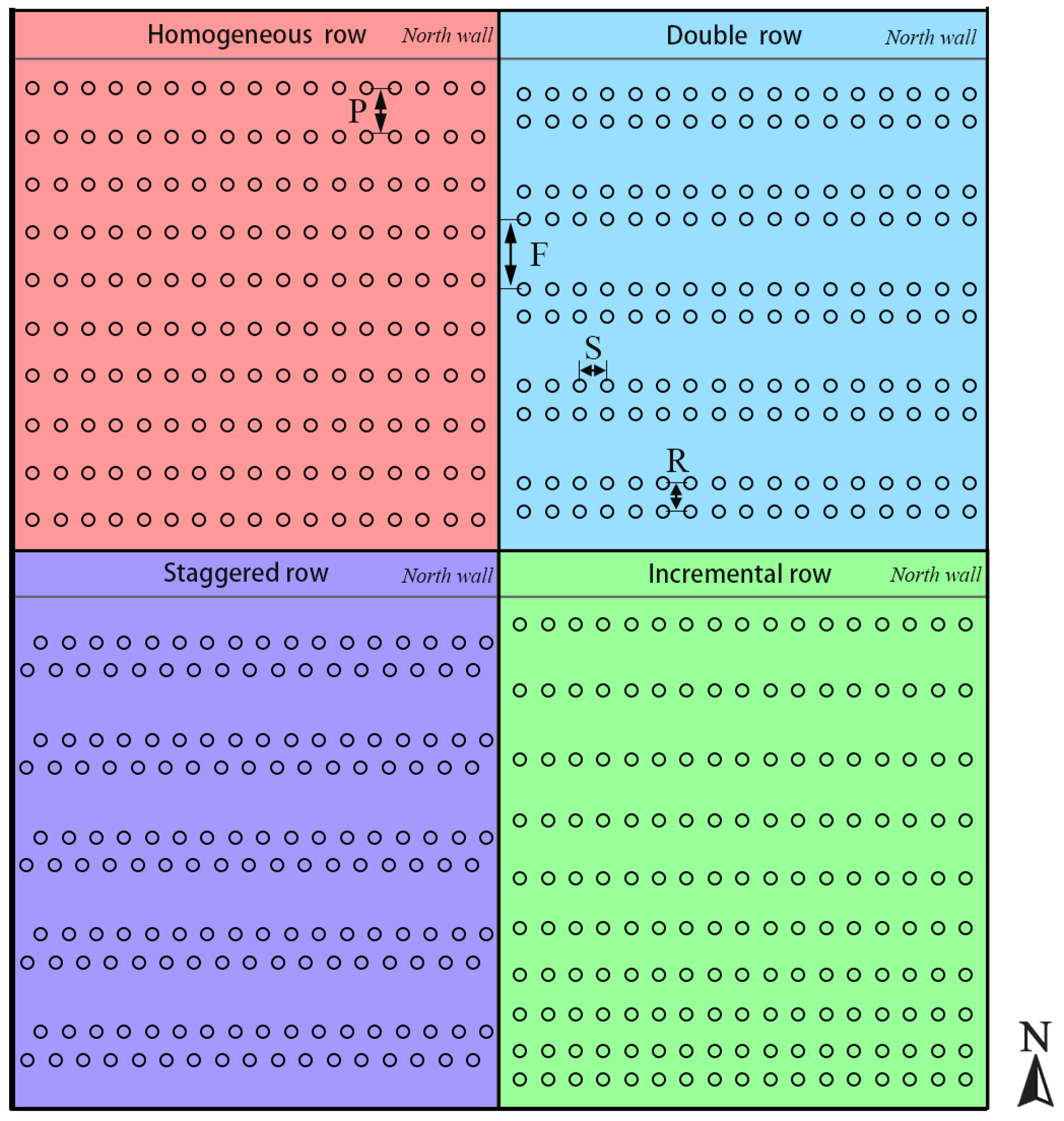
Simulation processes were run to calculate the radiation, temperature, and photosynthesis for each leaflet within a fully grown tomato canopy in the virtual greenhouse. Since the particular structure of the CSG leads to little difference between the east and west direction, and a greater difference between the north and south direction, a 15 m long virtual greenhouse was used for simulation. Climate data such as outdoor radiation, temperature, wind speed, and indoor CO2 concentration were used as inputs to run the model with half-hour time steps from 9:00 a.m. to 4:00 p.m. on winter solstice day (20 November 2019). For the configuration of the tomato canopy, the density was kept the same for all scenarios at 39,000 plants/ha, which is the widely used tomato planting density in CSG; for tomato mechanized planting the minimum row distance should be larger than 0.3 m and smaller than 1.6 m. Thus, in this study, the planting orientation was set to an E–W orientation with four treatments of furrow distance (1 m, 1.2 m, 1.4 m, 1.6 m). Each furrow distance treatment was then divided into four treatments of row spacing (0.3 m, 0.4 m, 0.5 m, 0.6 m). With the total plant density kept the same, each scenario had its corresponding planting configuration, as shown in Table 2. Each scenario was simulated with four planting patterns (homogeneous row, double row, staggered row, incremental row). The planting scenario with optimal performance was then selected and the N–S orientation with the same planting configuration was then simulated to compare the results.

2.3. Model Validation

The actual planting process was carried out in the Liaoshen solar greenhouse located at Shenyang Agricultural University (41°49′ N, 123°34′ E); the greenhouse has dimensions of 60 m length, 8 m span, and 4 m ridge height, with a 2.5 m height north wall and a roof projection of 1.5 m. The south side of the solar greenhouse is covered with plastic film. The tomato variety Shennong High Sugar Tomato-184 was used in this study. Tomato seedlings with four leaves were selected for field planting. The tomato crops were planted in N–S orientation with a furrow distance of 1 m, row spacing of 0.4 m, and plant spacing of 0.4 m. The daily management standard of tomato plants was kept the same for normal infinite-growth tomato cultivation management. The field cultivation management of each treated plant tomato group included single trunk pruning and a vertical hanging trellis, and when the plant grew to 1.8 m, the top was pinched. We measured outdoor and indoor temperature and humidity using temperature and relative humidity recorders (HOBO, U 23-001, Onset computer Corp., Bourne, MA, USA). We used a gas analyzer (LI-820; LI-COR, Lincoln, NE, USA) to measure indoor CO2 concentration. We connected thermocouples to a data logger (Fluke 2638 A HYDRA Series III Data Acquisition Unit, Fluke Corp., Valparaiso, IN, USA) to measure the temperatures of each LSG surface element, including the front cover, north wall, north roof, soil, and tomato leaflet. We used a photosynthesis system (LI-6800; LI-COR, Lincoln, NE, USA) with a red/blue LED light source (LI6800-02B) attached to a 6 cm2 clamp-on leaf chamber to measure photosynthetic-related parameters. Detailed model validation of the architecture module, light module, and photosynthesis module was conducted previously by [31]. All management methods and treatments were kept equal for all canopy configurations.

2.4. Statistical Analysis of Simulated Data

The simulated data for all canopy configurations were compiled into one single data file (CSV file) and further used to perform the partial least squares path modeling (PLS-PM) using SmartPLS 3.0 [32]. The PLS-PM analysis was used to investigate the connections between the simulated variables (such as furrow distance, plant distance, and planting pattern) through latent variables (e.g., canopy configuration, radiation, or photosynthesis) established by structural equation models. PLS–PM has been the predominant estimator for determining the relationships between latent variables with large-scale datasets for decades [33]. A total of 1000 bootstraps were performed during the simulation process of the PLS-PM to obtain R2 values of each latent variable and the path coefficients between them, which were determined by the confidence intervals and statistical significance. The path coefficients (i.e., standardized partial regression coefficients) function as the path direction and strength of the causal relationship between the indicators and their construct (direct effects). The connection between the predictor and response variable can be represented by indirect effects (multiplied coefficients) [34]. The physical and biological relationships of all simulated and latent variables were also considered to determine the optimal path model.

3. Results

3.1. Tomato Canopy Configuration Analysis for the Chinese Solar Greenhouse

The sixteen scenarios were simulated (Figure 2), each with four planting patterns (namely, homogeneous row, double row, staggered row, incremental row), and the modeling time was set for the winter solstice day (9:00 a.m. to 16:00 p.m.). Figure 3a shows the effect of increasing furrow distance on the pattern of plant intercepted radiation, which decreases sharply with increasing furrow distance while the plant density remains constant. The plant intercepted radiation also dropped as the row distance increased, but stopped decreasing after the row spacing was larger than 0.5 m (Figure 3b). As shown in Figure 3c, the plant intercepted radiation became higher as the plant spacing increased and stopped growing after 0.32 m (with a maximum plant light radiation mean value of 66.87 W m−2). Additionally, the 0.32 m plant spacing had the best uniformity among the last four treatments (the outlier data points with minimum values), i.e., 0.32 m, 0.34 m, 0.37 m, and 0.4 m. Therefore, for the planting density of 39,000 plants/ha, a 0.32 m plant spacing is the best solution, and there are two scenarios corresponding to the 0.32 m plant spacing, e.g., scenario 4 (F = 1 m, R = 0.6 m) and scenario 6 (F = 1.2 m, R = 0.4 m). Comparing the F and R of these two scenarios in Figure 3a,b, we can infer that the combination of F = 1.2 m, R = 0.4 m (scenario 6) has a slightly better influence on the light interception than that of scenario 4 (66.10 W m−2 to 65.9 W m−2). By comparing within the group of scenario 6, planting pattern 1 (homogeneous row) has the overall best radiation performance (plant average light interception = 67.36 W m−2, Figure 3c).
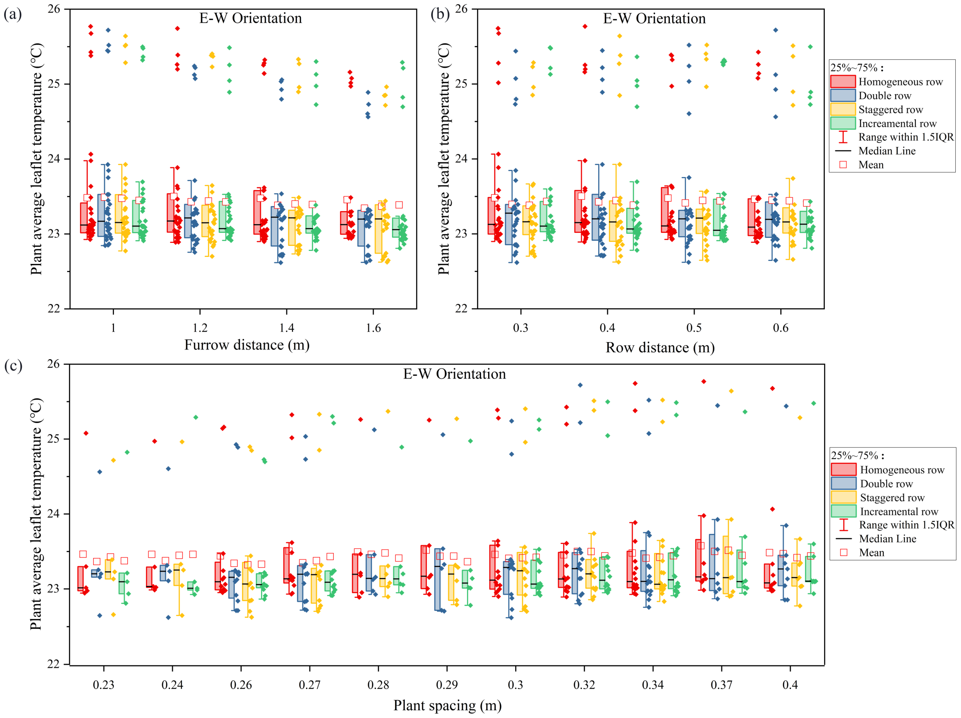
Leaf photosynthetic rates cannot be accurately assessed by leaf light alone, so leaf temperature calculations are needed to fully assess complex greenhouse plant interactions. The plant average leaf temperature was calculated for each scenario of the four planting patterns and is depicted in Figure 4. As Figure 4 shows, the plant leaf temperature dropped as the furrow distance and row distance increased, and plant leaf temperature became higher with increasing plant spacing and started decreasing after 0.37 m (average leaf temperature = 23.5 °C). Therefore, the best plant temperature performance for the planting density of 39,000 plants/ha is the 0.37 m plant spacing of scenario 2 (F = 1 m, R = 0.4 m).
As shown in Figure 5a, with the plant density kept equal to 39,000 plants/ha, the effect of furrow distance on plant photosynthesis reached its peak value at 1.2 m (plant average photosynthesis rate = 8.65 μmol m−2 s−1). The effect of row distance reaches the maximum at a 0.4 m row distance Figure 5b (plant average photosynthesis rate = 8.62 μmol m−2 s−1). The effects of plant spacing on mean photosynthesis rate reach the maximum at 0.32 m (with the highest plant light radiation mean value of 8.87 μmol m−2 s−1). In summary, the best photosynthetic performance of plant leaves was observed in scenario 6 (F = 1.2 m, R = 0.4 m, S = 0.32 m) compared to the other scenarios. By comparing within the group of scenario 6, planting pattern 1 (homogeneous row) had the best photosynthesis performance overall, with the highest mean photosynthesis rate and best uniformity (Figure 5c).

3.2. Comparing the Optimum Canopy Configuration of E–W Orientation with N–S Orientation

The E–W orientation of scenario 6 was then selected (based on the results from Figure 3, Figure 4 and Figure 5) to compare the detailed difference with the same canopy configuration of N–S scenarios. Figure 6 indicates the plant solar radiation performance for scenario 6 in both orientations during the day (four planting patterns). Due to the special structure of the Chinese solar greenhouse’s front cover, tomato plants located at the southern part of the canopy can intercept significantly higher radiation than those at the central and northern parts, especially for the southern front row. According to the data, the E–W orientation intercepted more solar radiation in the central and northern parts of the canopy compared to the N–W orientation. However, in the two row and staggered row systems, the row facing north is clearly obscured.
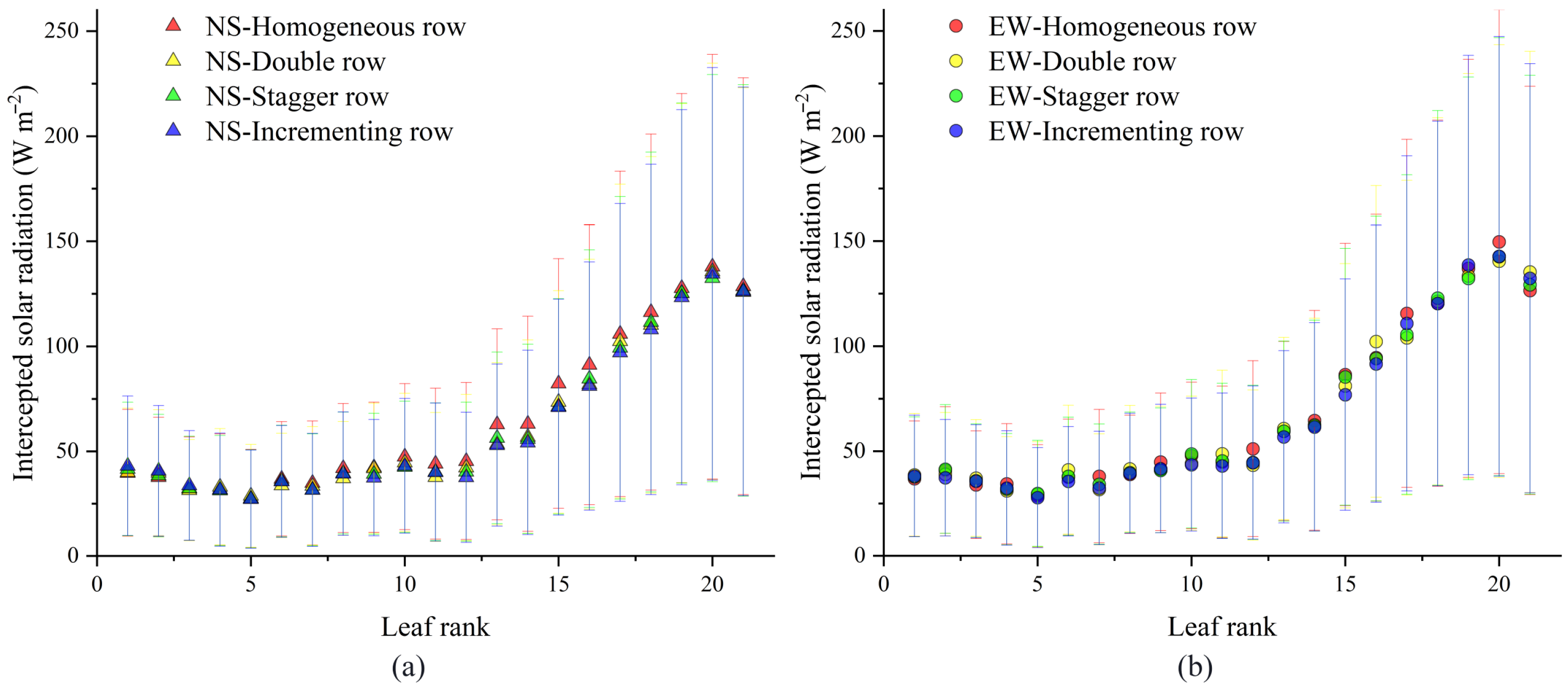
The plant-level radiation alone would not be sufficient to clearly illustrate the main difference between the two orientations, which also makes it difficult to find the optimal configuration. Thus, the leaf-level radiation was further compared to address this problem. Figure 7 shows the daily average solar radiation intercepted at each leaf rank for the eight above-mentioned patterns. The homogeneous row pattern in the N–S orientation showed a significantly higher amount of radiation on multiple leaf ranks (leaf ranks 7, 8, 10, 11, 12, 13, 14, 15, 16, 17, 18, 19, 20, and 21) (Figure 7a), and the same pattern also performs slightly better radiation interception in the E–W orientation at leaf ranks 4, 7, 9, 12, 14, 15, 17, and 20. The homogeneous row pattern performed better in both orientations at the furrow distance of 1.2 m, row distance of 0.4 m, and plant spacing of 0.32 m, and plant density of 39,000 plants/ha.
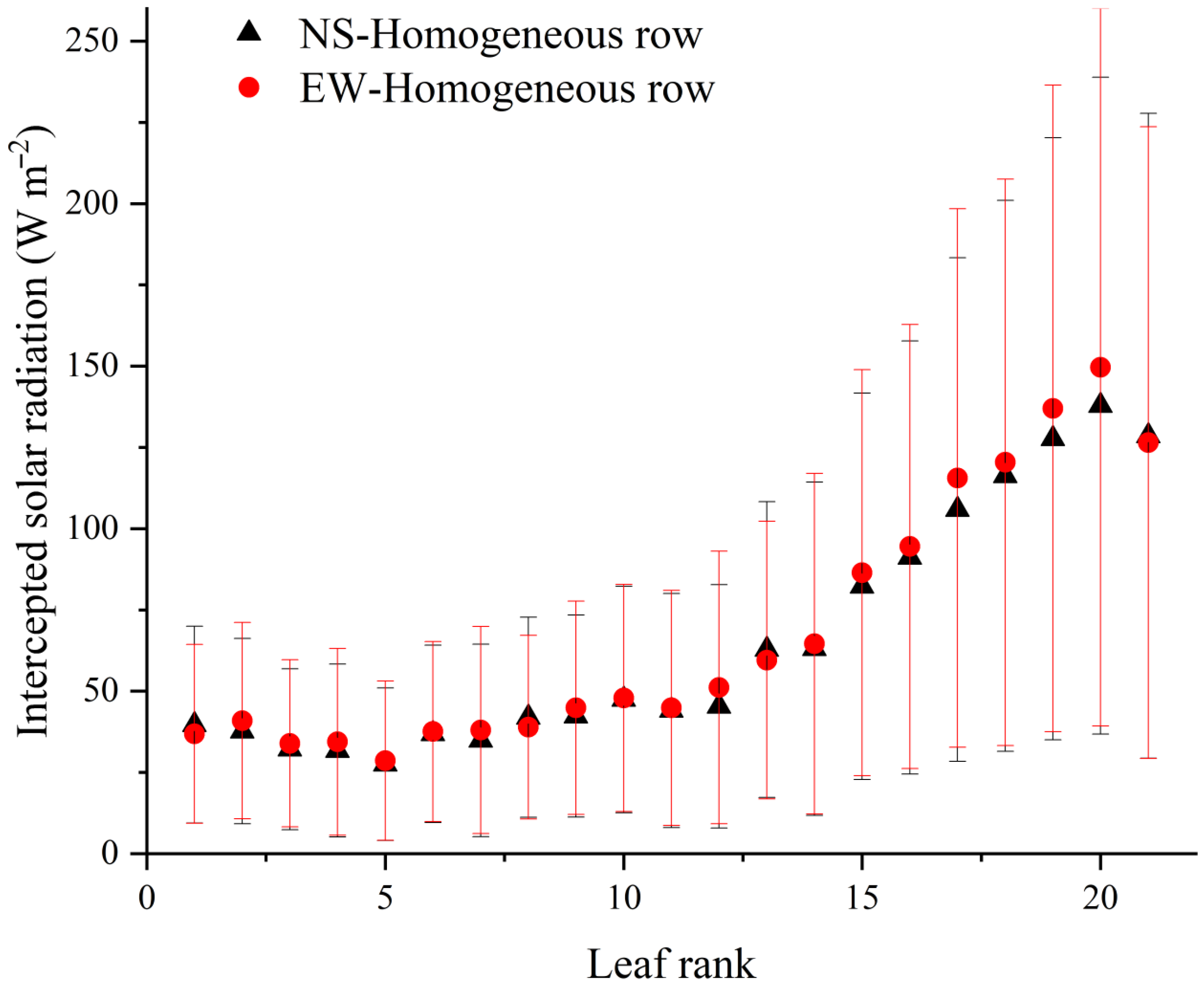
The homogeneous row with two orientations was singled out to compare the intercepted radiation on each leaf rank in Figure 8. Results indicated that the E–W orientation showed a clearly higher value of solar radiation compared to the most used N–S orientation on most leaf ranks (2, 3, 4, 5, 6, 7, 9, 12, 15–20).
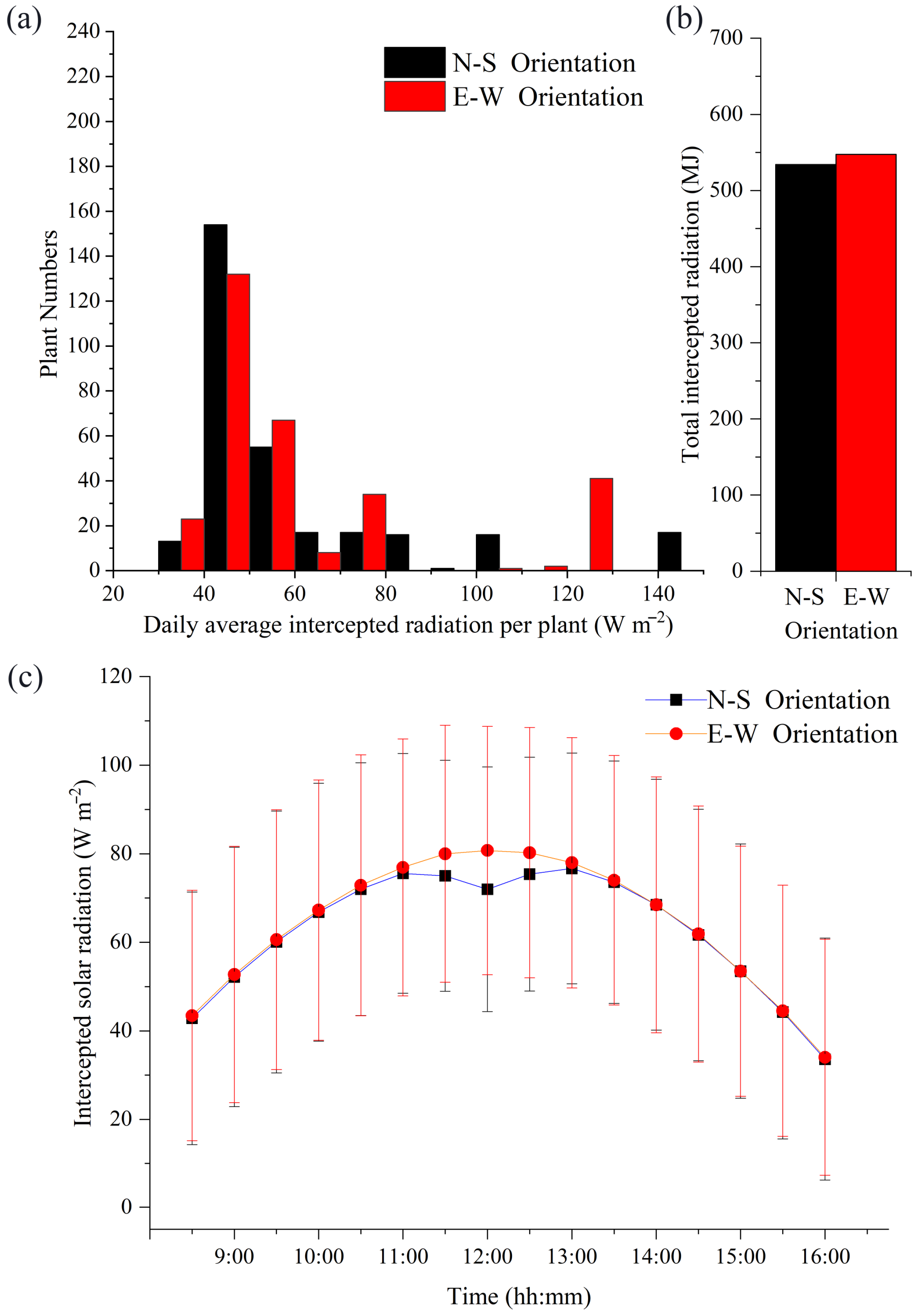
To determine why the E–W orientation in scenario 6 has a better daily light interception effect than that of the N–S orientation, we performed statistical analysis of these two orientations. Figure 9a shows that in the scenario 6 configuration, the E–W orientation has better uniformity in terms of plant numbers than the N–S orientation, with the E–W orientation plants showing mostly medium range radiation levels (45–130 W m−2), while on the other hand, the N–S orientation has more plants at radiation levels of 40 W m−2 and 140 W m−2. The daily total radiation in the E–W orientation is also better than that of the N–S orientation (Figure 9b). The higher radiation of the E–W orientation mainly comes from the midday time zone (11:00 a.m.–1:00 p.m.), where the horizontal direction of sunlight is direct from south to north. This is directly in line with the canopy direction of N–S, which will result in more self-shading of the plants than the E–W orientation.
Photosynthesis is the basic way for crops to obtain organic matter and energy; however, although photosynthesis is mainly driven by light, we still need to compare the differences in photosynthesis due to the non-linear response of photosynthesis to light [35]. Thus, we further compared the two orientations under the homogeneous row of scenario 6 (P = 0.8 m, S = 0.32 m).
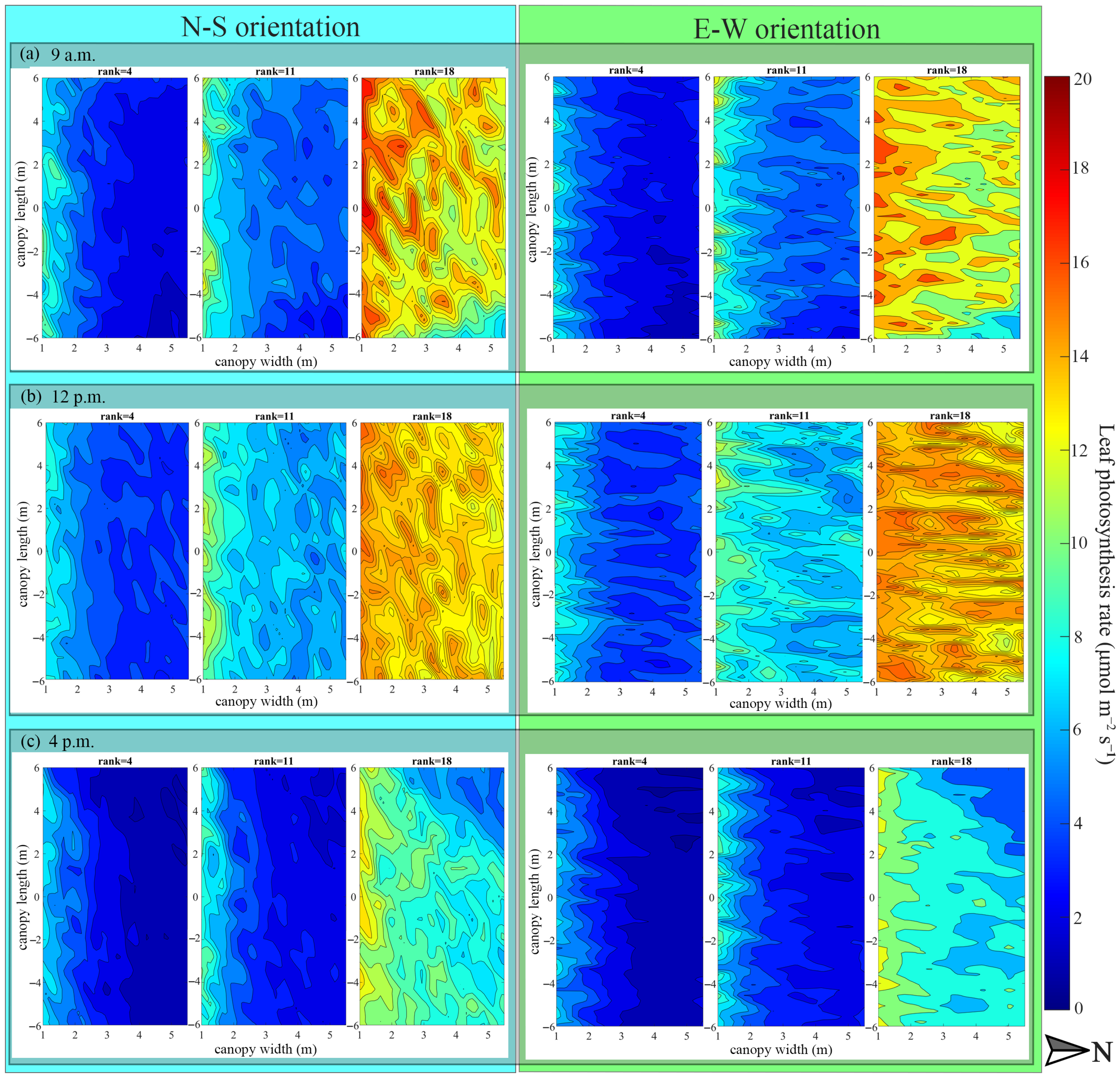
The heat maps in Figure 10 depict the distribution of the photosynthesis rate in the upper (leaf rank = 18), middle (leaf rank = 11), and lower (leaf rank = 4) layers of the tomato canopy at three time points (9:00 a.m., 12:00 p.m., and 4:00 p.m.). The N–S orientation upper canopy showed higher photosynthesis rate values in the northern part of the greenhouse compared to the E–W orientation; however, the middle layer leaves of the E–W orientation were slightly better than those of the N–S orientation during the morning period (9:00 a.m.). Around noon (11:00 a.m.–1:00 p.m.), better photosynthetic rates and photosynthetic uniformity could be achieved in the upper and middle canopies in the E–W orientation under scenario 6 (P = 0.8 m, S = 0.32 m) compared to the N–S orientation. This outcome also corresponds to Figure 9c; at midday, the horizontal component of the direct sun rays shines directly from the southern side of the greenhouse to the north, which is in a straight line with the N–S orientation canopy. This will cause more inter-plant shading inside the canopy than in the E–W orientation. At sunset, the photosynthesis performance in the N–S orientation performed slightly better than photosynthesis in the E–W orientation at late afternoon, i.e., 4 o’clock.
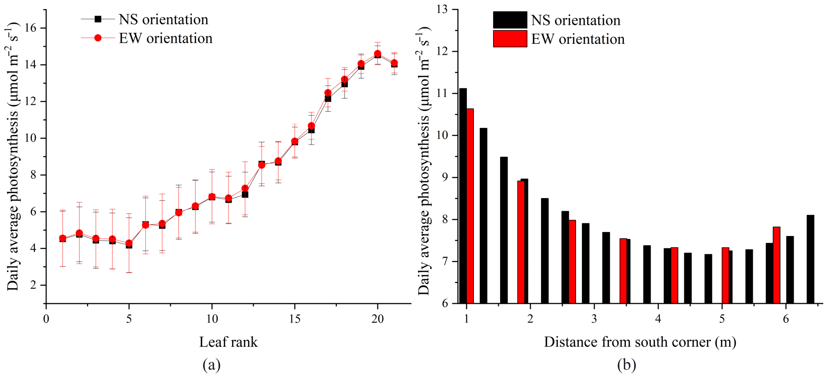
To conclude, both orientations in scenario 6 had to be compared by means of data analysis to assess their detailed photosynthesis performance. Thus, we compared the daily average photosynthesis of each leaf rank in both orientations, as shown in Figure 11. As can be seen from Figure 11a, the E–W orientation performed slightly better in terms of the daily average photosynthesis rate than the N–S orientation on leaf ranks 2, 3, 4, 5, 7, 11, 12, 14, 16, 17, 18, 19, 20, and 21. Figure 11b describes the daily photosynthesis performance of middle lane plants of both orientations. The E–W orientation showed a clearly higher photosynthesis rate on the north part of the canopy (6 m from the south corner) because the 6 m point is where the plants are closest to the wall in the E–W direction, and the reflection and scattering effect of the north wall on light causes the marginal row of plants to receive more light than the middle plants. This leads to the conclusion that scenario 6 with the E–W orientation (F = 1.2 m, RD = 0.4 m, S = 0.32 m) is the most suitable canopy configuration for CSG mechanized planting at the most used plant density of 39,000 plants/ha.

3.3. Partial Least Squares Path Modeling Analysis (PLS-PM)

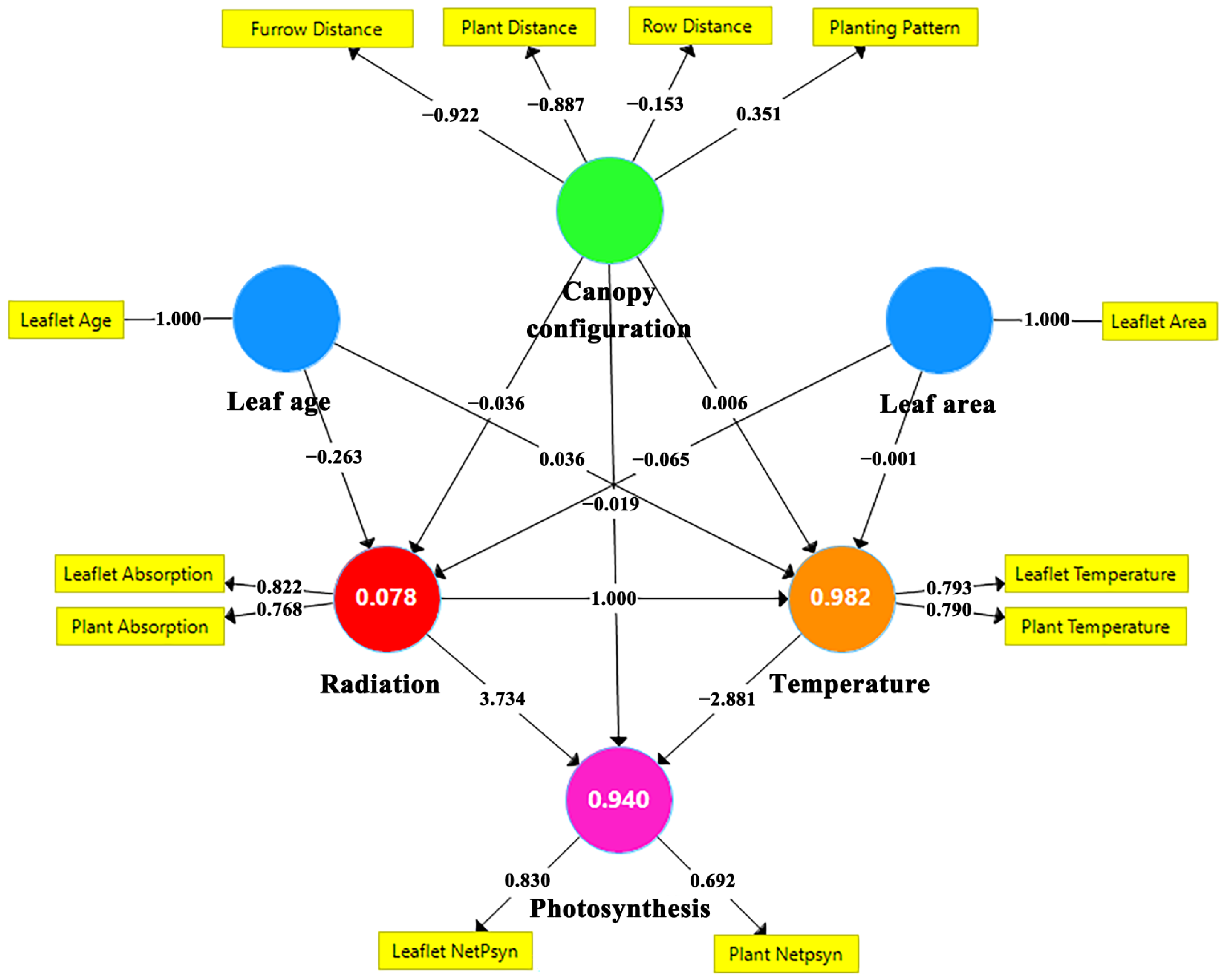
To further strengthen the generalizability of this study, the PLS–PM analysis was performed to comprehend how all the above-simulated E–W orientation scenario traits (furrow distance, row distance, plant distance, planting pattern, leaflet age, leaflet area, leaf absorption, leaf temperature, leaf photosynthesis) are interrelated and their causal relationship [36]. During the modeling process, simulated variables with physical and biological connections were combined into a latent variable (e.g., canopy configuration), and thus the simulated and latent variables form the outer model (for outer loadings please refer to Supplementary Table S2). The inner model was created for the study of relationships between latent variables, and the linkages for the inner model were represented by path coefficients (Supplementary Table S3). R2 was also used to serve as the measure of how well the specific latent variable is represented by other endogenous latent values (Supplementary Table S4).
The modeling result showed that canopy configuration had relatively small effects on radiation, temperature, and photosynthesis, with only an indirect effect value of −0.133 of canopy configuration on photosynthesis, which was mediated by the radiation (Supplementary Table S5). The canopy configuration was well represented by the furrow distance (0.922), plant distance (−0.87), and planting pattern (0.351). However, the row distance has an insignificant effect on representing the canopy configuration (0.153) (Figure 12). Since the effect of canopy configuration on radiation and photosynthesis was negative (−0.036 and −0.019), increasing the value of the furrow distance, row distance, and plant pattern will negatively affect plant interception of radiation and photosynthesis while plant density remains constant. On the other hand, increasing the plant distance will have a positive effect on plant radiation and photosynthesis. This result corresponds well with the former results of Figure 3 and Figure 5.

4. Discussion

4.1. Changing from the Widely Used N–S Orientation to the E–W Orientation

A comprehensive analysis of major trends in the evolution of planting strategies suitable for Chinese solar greenhouses was conducted by [37]. Despite this, a planting strategy specifically optimized for the cultivation conditions of Chinese solar greenhouses in the northern region remains unidentified. This study aimed to address this gap by investigating the optimal canopy configuration that maximizes light capture and photosynthetic performance in Chinese solar greenhouses. This was achieved using a virtual solar greenhouse and a tomato plant canopy model. In the current modeling study, to effectively compare the differences between orientations and identify the optimal configuration for east–west planting, other modeling configurations such as tomato growth stages, planting density, greenhouse locations, and the surrounding environment were kept constant. Future studies will focus on identifying the effects of these other factors on canopy photosynthesis.
The results revealed only a minimal difference in daily light absorption and net photosynthesis between north–south and east–west orientations (Figure 8). This finding aligns with article [15], which reported similar light absorption and net photosynthesis across different row orientations. This is also consistent with the model simulations of [38], who suggested that row orientation has less influence at higher latitudes when the path width and row height ratio is ≤30%. Although the differences between different row orientations are small, due to the daily average calculations in this study, even small differences can be amplified over time.

4.2. The Optimal Configuration of E–W Orientation Has Been Identified

The simulation data showed that scenario 6 with the planting pattern 1 (homogeneous row) had the best overall radiation performance, the best plant temperature performance with a planting density of 39,000 plants/ha was in the homogeneous row of scenario 2 (Figure 4), and the optimal photosynthesis performance also occurred in scenario 6 with planting pattern 1 (Figure 5). Previous studies [15,39] investigated interrow shading in an east–west double row orientation. These findings also showed that a homogeneous row exhibits superior performance compared to a double row in an east–west orientation. This outcome was also demonstrated by comparing the E–W orientation of scenario 6 with the N–S orientation, where the daily light interception, temperature, and photosynthesis were compared in detail on a per-leaf basis, showing that the E–W orientation of scenario 6 performed better in terms of light interception for the upper leaf rank (Figure 8), plant numbers (Figure 9a), and at midday (Figure 9c). The primary objective of investigating the optimal plant arrangement is to minimize shading. It has been reported that canopy shading can negatively impact flower bud formation, fruit set, and fruit quality in horticultural crops [40]. Regarding photosynthesis, the E–W orientation showed better photosynthesis in the upper-middle and northern parts of the canopy (Figure 10). Overall, in practice, it is better to use homogeneous rows in the E–W orientation of scenario 6, which is also more suitable for mechanized planting.

4.3. Similar Trends Can Be Applied for Other Planting Configurations

Previous research found vertical profiles of tomato photosynthesis and yield, highlighting the importance of irradiance on the photosynthesis and yield [41]. Here we have shown and modeled distinct patterns of incident irradiance, temperature, and photosynthesis for N–S and E–W oriented ridges and advanced knowledge regarding the interactions among plant leaf irradiance, temperature, and photosynthesis. The result of PLS-PM showed that if the planting density is kept at 39,000 plants/ha, increasing the values of the furrow distance, row distance, and planting pattern will negatively affect plant interception of radiation and photosynthesis, although the effect of canopy configuration on radiation, temperature, and photosynthesis is relatively small. Increasing the plant distance, on the other hand, will have a positive effect on plant radiation and photosynthesis. It was concluded from PLS-PM observations that, instead of increasing furrow or row spacing, plant spacing should be increased to some extent and furrow distance should be reduced to achieve better absorption in the tomato canopy within the CSG when plant density in the E–W oriented tomato canopy is not changed. Comparable patterns can be utilized for different greenhouse planting arrangements.

5. Conclusions

In conclusion, our study on the optimal canopy configuration for east–west (E–W) oriented planting in Chinese solar greenhouses has provided valuable insights into the mechanistic links between canopy traits and tomato leaf physiology. Through comprehensive virtual greenhouse simulations encompassing various furrow distances, row spacings, and plant spacings, we aimed to address our hypothesis regarding the ideal configuration to maximize radiation and photosynthesis performance. Our findings reveal that, for the E–W orientation, a planting density of 39,000 plants/ha, a furrow distance of 1.2 m, and a row distance of 0.4 m collectively optimize leaflet radiation, temperature, and photosynthesis. Notably, a plant spacing of 0.32 m emerges as the key factor for achieving uniform photosynthesis. Comparison with the north–south (N–S) orientation underscores the superior performance of the E–W orientation, particularly in the northern and upper-middle canopy regions. The significance of our results lies in their direct applicability to mechanized planting practices. The recommended configuration, characterized by a homogeneous row with a path distance (P) of 0.8 m and a plant distance of 0.32 m, represents an efficient solution for solar greenhouse cultivation. This mechanistic approach aligns with our initial hypothesis, emphasizing the importance of specific canopy traits in enhancing light environment and photosynthesis rates. In terms of novelty, our study contributes to the existing literature by elucidating the nuanced interplay between canopy configuration and plant physiology. The implications of these findings extend beyond the immediate context of the E–W orientation, offering actionable insights for optimizing productivity in solar greenhouses and providing clear strategies for transitioning from the N–S orientation to the E–W orientation during mechanized ridging. In essence, the mechanistic links identified in this study underscore the practical applicability of our findings, positioning them as a valuable resource for greenhouse farmers, researchers, and practitioners alike. As we move forward, these conclusions not only answer the core hypothesis of our study but also pave the way for future research endeavors aimed at refining and expanding our understanding of optimal canopy management in greenhouse environments.

Supplementary Materials

The following supporting information can be downloaded at: https://www.mdpi.com/article/10.3390/agronomy14020249/s1, Table S1: Equations of the modules for energy balance, photosynthesis, and stomatal conductance; Table S2: Outer model loadings and significance. Original and sample mean for each simulated variable are shown, with standard deviation and p-values; Table S3: The path coefficients between the latent variables. Original and sample mean between each two latent variables are shown, with standard deviation and p-values; Table S4: R2 values for each latent variable in the inner model. Original and sample mean values and R2 values; Table S5: Specific indirect effects between the latent variables. Original and sample mean for each indirect path are shown, with standard deviation and p-values.

Author Contributions

Y.Z., M.H., X.L. and T.L. planned and designed the research; Y.Z. performed experiments and conducted fieldwork; M.H. provided methodology and software; Y.Z. and M.H. implemented the models, analyzed the data, and wrote the manuscript; M.H., Y.L., Z.S., W.L., X.L. and T.L. reviewed and edited the manuscript; X.L. acquired the funding; T.L. supervised the project. All authors have read and agreed to the published version of the manuscript.

Funding

This work was supported by the Applied Basic Research Programs of Shanxi Province (202203021222295); the China Agriculture Research System (CARS-23); the Science and Technology Innovation Project of Higher Education Institutions in Shanxi Province (2022L456, 2021L398); the Applied Basic Research Programs of Datong City (2023063); the Basic Research Programs of Shanxi Datong University (2022K25); and the Doctoral Research Project of Shanxi Datong University (2022-B-03).

Data Availability Statement

Data are contained within the article and supplementary materials.

Acknowledgments

We would like to express our gratefulness to Gerhard H. Buck-Sorlin for the selfless help and guidance on the photosynthesis model.

Conflicts of Interest

The authors declare no conflicts of interest.

References

  1. He, X.; Qiao, Y.; Liu, Y.; Dendler, L.; Yin, C.; Martin, F. Environmental Impact Assessment of Organic and Conventional Tomato Production in Urban Greenhouses of Beijing City, China. J. Clean. Prod. 2016, 134, 251–258. [Google Scholar] [CrossRef]
  2. Zhang, Y.; Henke, M.; Li, Y.; Yue, X.; Xu, D.; Liu, X.; Li, T. High Resolution 3D Simulation of Light Climate and Thermal Performance of a Solar Greenhouse Model under Tomato Canopy Structure. Renew. Energy 2020, 160, 730–745. [Google Scholar] [CrossRef]
  3. Meiyan, W. The Rise of Labor Cost and the Fall of Labor Input: Has China Reached Lewis Turning Point? China Econ. J. 2010, 3, 137–153. [Google Scholar] [CrossRef]
  4. Zheng, L.; Zhang, Q.; Zheng, K.; Zhao, S.; Wang, P.; Cheng, J.; Zhang, X.; Chen, X. Effects of Diffuse Light on Microclimate of Solar Greenhouse, and Photosynthesis and Yield of Greenhouse-Grown Tomatoes. HortScience 2020, 55, 1605–1613. [Google Scholar] [CrossRef]
  5. Ouyang, Z.; Tian, J.; Yan, X.; Shen, H. Photosynthesis, Yield and Fruit Quality of Tomatoes and Soil Microorganisms in Response to Soil Temperature in the Greenhouse. Irrig. Drain. 2022, 71, 604–618. [Google Scholar] [CrossRef]
  6. Liu, N.; Wei, Z.; Wei, H. The Effect of Planting Mode on the Growth of Pepper in a Sunlight Greenhouse. IOP Conf. Ser. Earth Environ. Sci. 2021, 692, 032001. [Google Scholar] [CrossRef]
  7. Dong, Q.; Louarn, G.; Wang, Y.; Barczi, J.F.; De Reffye, P. Does the Structure-Function Model GREENLAB Deal with Crop Phenotypic Plasticity Induced by Plant Spacing? A Case Study on Tomato. Ann. Bot. 2008, 101, 1195–1206. [Google Scholar] [CrossRef]
  8. Wang, J.; Li, S.; Guo, S.; Ma, C.; Wang, J.; Jin, S. Simulation and Optimization of Solar Greenhouses in Northern Jiangsu Province of China. Energy Build. 2014, 78, 143–152. [Google Scholar] [CrossRef]
  9. Amare, G.; Gebremedhin, H. Effect of Plant Spacing on Yield and Yield Components of Tomato (Solanum lycopersicum L.) in Shewarobit, Central Ethiopia. Scientifica 2020, 2020, 8357237. [Google Scholar] [CrossRef]
  10. Ohashi, Y.; Torii, T.; Ishigami, Y.; Goto, E. Estimation of the Light Interception of a Cultivated Tomato Crop Canopy under Different Furrow Distances in a Greenhouse Using the Ray Tracing. J. Agric. Meteorol. 2020, 76, 188–193. [Google Scholar] [CrossRef]
  11. Schipper, R.; van der Meer, M.; de Visser, P.H.B.; Heuvelink, E.; Marcelis, L.F.M. Consequences of Intra-Canopy and Top LED Lighting for Uniformity of Light Distribution in a Tomato Crop. Front. Plant Sci. 2023, 14, 1012529. [Google Scholar] [CrossRef] [PubMed]
  12. Bielczynski, L.W.; Łaçki, M.K.; Hoefnagels, I.; Gambin, A.; Croce, R. Leaf and Plant Age Affects Photosynthetic Performance and Photoprotective Capacity. Plant Physiol. 2017, 175, 1634–1648. [Google Scholar] [CrossRef] [PubMed]
  13. Mohammed, H.A.; Aljabary, A.M.A.O.; Halshoy, H.S.; Hama, J.R.; Rashid, H.A.; Rashid, H.W. Soil-Borne Microbes, Natural Stimulants, and Post-Harvest Treatments Alter Quality and Phytochemicals of Tomato Fruit. Int. J. Veg. Sci. 2023, 1–13. [Google Scholar] [CrossRef]
  14. Niinemets, Ü. Photosynthesis and Resource Distribution through Plant Canopies. Plant Cell Environ. 2007, 30, 1052–1071. [Google Scholar] [CrossRef] [PubMed]
  15. van der Meer, M.; de Visser, P.H.B.; Heuvelink, E.; Marcelis, L.F.M. Row Orientation Affects the Uniformity of Light Absorption, but Hardly Affects Crop Photosynthesis in Hedgerow Tomato Crops. Silico Plants 2021, 3, diab025. [Google Scholar] [CrossRef]
  16. Berrueta, C.; Borges, A.; Giménez, G.; Dogliotti, S. On-Farm Diagnosis for Greenhouse Tomato in South Uruguay: Explaining Yield Variability and Ranking of Determining Factors. Eur. J. Agron. 2019, 110, 125932. [Google Scholar] [CrossRef]
  17. Kimura, K.; Yasutake, D.; Koikawa, K.; Kitano, M. Spatiotemporal Variability of Leaf Photosynthesis and Its Linkage with Microclimates across an Environment-Controlled Greenhouse. Biosyst. Eng. 2020, 195, 97–115. [Google Scholar] [CrossRef]
  18. Wang, W.M.; Li, Z.L.; Su, H.B. Comparison of Leaf Angle Distribution Functions: Effects on Extinction Coefficient and Fraction of Sunlit Foliage. Agric. For. Meteorol. 2007, 143, 106–122. [Google Scholar] [CrossRef]
  19. Vose, J.M.; Clinton, B.D.; Sullivan, N.H.; Bolstad, P.V. Vertical Leaf Area Distribution, Light Transmittance, and Application of the Beer–Lambert Law in Four Mature Hardwood Stands in the Southern Appalachians. Can. J. For. Res. 1995, 25, 1036–1043. [Google Scholar] [CrossRef]
  20. Vos, J.; Evers, J.B.; Buck-Sorlin, G.H.; Andrieu, B.; Chelle, M.; de Visser, P.H.B. Functional-Structural Plant Modelling: A New Versatile Tool in Crop Science. J. Exp. Bot. 2010, 61, 2101–2115. [Google Scholar] [CrossRef]
  21. Gao, Y.; Dong, J.; Isabella, O.; Santbergen, R.; Tan, H.; Zeman, M.; Zhang, G. Modeling and Analyses of Energy Performances of Photovoltaic Greenhouses with Sun-Tracking Functionality. Appl. Energy 2019, 233–234, 424–442. [Google Scholar] [CrossRef]
  22. Sarlikioti, V.; de Visser, P.H.B.; Marcelis, L.F.M. Exploring the Spatial Distribution of Light Interception and Photosynthesis of Canopies by Means of a Functionalstructural Plant Model. Ann. Bot. 2011, 107, 875–883. [Google Scholar] [CrossRef] [PubMed]
  23. van der Meer, M.; Lee, H.; de Visser, P.H.B.; Heuvelink, E.; Marcelis, L.F.M. Consequences of Interplant Trait Variation for Canopy Light Absorption and Photosynthesis. Front. Plant Sci. 2023, 14, 1012718. [Google Scholar] [CrossRef] [PubMed]
  24. Soualiou, S.; Wang, Z.; Sun, W.; de Reffye, P.; Collins, B.; Louarn, G.; Song, Y. Functional–Structural Plant Models Mission in Advancing Crop Science: Opportunities and Prospects. Front. Plant Sci. 2021, 12, 747142. [Google Scholar] [CrossRef] [PubMed]
  25. Albasha, R.; Fournier, C.; Pradal, C.; Chelle, M.; Prieto, J.A.; Louarn, G.; Simonneau, T.; Lebon, E. HydroShoot: A Functional-Structural Plant Model for Simulating Hydraulic Structure, Gas and Energy Exchange Dynamics of Complex Plant Canopies under Water Deficit—Application to Grapevine (Vitis vinifera). Silico Plants 2019, 1, diz007. [Google Scholar] [CrossRef]
  26. Chen, T.W.; Nguyen, T.M.N.; Kahlen, K.; Stützel, H. Quantification of the Effects of Architectural Traits on Dry Mass Production and Light Interception of Tomato Canopy under Different Temperature Regimes Using a Dynamic Functional-Structural Plant Model. J. Exp. Bot. 2014, 65, 6399–6410. [Google Scholar] [CrossRef] [PubMed]
  27. Evers, J.B.; Vos, J.; Yin, X.; Romero, P.; Van Der Putten, P.E.L.; Struik, P.C. Simulation of Wheat Growth and Development Based on Organ-Level Photosynthesis and Assimilate Allocation. J. Exp. Bot. 2010, 61, 2203–2216. [Google Scholar] [CrossRef] [PubMed]
  28. Auzmendi, I.; Hanan, J.S. Investigating Tree and Fruit Growth through Functional-Structural Modelling: Implications of Carbon Autonomy at Different Scales. Ann. Bot. 2020, 126, 775–788. [Google Scholar] [CrossRef]
  29. Tang, L.; Yin, D.; Chen, C.; Yu, D.; Han, W. Optimal Design of Plant Canopy Based on Light Interception: A Case Study with Loquat. Front. Plant Sci. 2019, 10, 364. [Google Scholar] [CrossRef]
  30. Kniemeyer, O. Design and Implementation of a Graph Grammar Based Language for Functional-Structural Plant Modelling. Ph.D. Thesis, BTU Cottbus, Senftenberg, Germany, November 2008; p. 432. [Google Scholar]
  31. Zhang, Y.; Henke, M.; Buck-Sorlin, G.H.; Li, Y.; Xu, H.; Liu, X.; Li, T. Estimating Canopy Leaf Physiology of Tomato Plants Grown in a Solar Greenhouse: Evidence from Simulations of Light and Thermal Microclimate Using a Functional-Structural Plant Model. Agric. For. Meteorol. 2021, 307, 108494. [Google Scholar] [CrossRef]
  32. Ringle, C.M.; Wende, S.; Becker, J.-M. SmartPLS 3; Boenningstedt SmartPLS GmbH: Boenningstedt, Germany, 2015. [Google Scholar]
  33. Rowland, S.D.; Zumstein, K.; Nakayama, H.; Cheng, Z.; Flores, A.M.; Chitwood, D.H.; Maloof, J.N.; Sinha, N.R. Leaf Shape Is a Predictor of Fruit Quality and Cultivar Performance in Tomato. New Phytol. 2020, 226, 851–865. [Google Scholar] [CrossRef] [PubMed]
  34. Barberán, A.; Ramirez, K.S.; Leff, J.W.; Bradford, M.A.; Wall, D.H.; Fierer, N. Why Are Some Microbes More Ubiquitous than Others? Predicting the Habitat Breadth of Soil Bacteria. Ecol. Lett. 2014, 17, 794–802. [Google Scholar] [CrossRef] [PubMed]
  35. Kohli, A.; Miro, B.; Balié, J.; d’A Hughes, J. Photosynthesis Research: A Model to Bridge Fundamental Science, Translational Products, and Socio-Economic Considerations in Agriculture. J. Exp. Bot. 2020, 71, 2281–2298. [Google Scholar] [CrossRef] [PubMed]
  36. Granier, C.; Vile, D. Phenotyping and beyond: Modelling the Relationships between Traits. Curr. Opin. Plant Biol. 2014, 18, 96–102. [Google Scholar] [CrossRef] [PubMed]
  37. Zhang, Y.; Henke, M.; Li, Y.; Xu, D.; Liu, A.; Liu, X.; Li, T. Analyzing the Impact of Greenhouse Planting Strategy and Plant Architecture on Tomato Plant Physiology and Estimated Dry Matter. Front. Plant Sci. 2022, 13, 828252. [Google Scholar] [CrossRef]
  38. Gijzen, H.; Goudriaan, J. A Flexible and Explanatory Model of Light Distribution and Photosynthesis in Row Crops. Agricultural. Agric. For. Meteorol. 1989, 48, 1–20. [Google Scholar] [CrossRef]
  39. Trentacoste, E.R.; Gómez-del-Campo, M.; Rapoport, H.F. Olive Fruit Growth, Tissue Development and Composition as Affected by Irradiance Received in Different Hedgerow Positions and Orientations. Sci. Hortic. 2016, 198, 284–293. [Google Scholar] [CrossRef]
  40. Trentacoste, E.R.; Connor, D.J.; Gómez-del-Campo, M. Row Orientation: Applications to Productivity and Design of Hedgerows in Horticultural and Olive Orchards. Sci. Hortic. 2015, 187, 15–29. [Google Scholar] [CrossRef]
  41. Sarlikioti, V.; De Visser, P.H.B.; Buck-Sorlin, G.H.; Marcelis, L.F.M. How Plant Architecture Affects Light Absorption and Photosynthesis in Tomato: Towards an Ideotype for Plant Architecture Using a Functionalstructural Plant Model. Ann. Bot. 2011, 108, 1065–1073. [Google Scholar] [CrossRef]
Figure 1. Photograph of a real CSG (Liaoshen type) (a). Three-dimensional model of a 15 m long Chinese Liaoshen solar greenhouse including the tomato canopy with E–W row orientation (b). The 15 m long version of the greenhouse was used to simulate all scenarios, which can significantly reduce the calculation time and has no impact on the overall simulated results (the CSG has 60 m length).
Agronomy 14 00249 g001
Figure 2. Schematic representation of the E–W row orientation with four trellis patterns, namely, homogeneous, double row, staggered, and incremental row. E.g., F: furrow distance, R: row distance, S: plant spacing, P: (furrow distance + row distance)/2.
Agronomy 14 00249 g002
Figure 3. The daily average plant incident solar radiation under four planting patterns of E–W orientation as the furrow distance (a), row distance (b), and plant distance (c) increases.
Agronomy 14 00249 g003
Figure 4. The midday plant average leaflet temperature under four planting patterns of E–W orientation as the furrow distance (a), row distance (b), and plant distance (c) increases.
Agronomy 14 00249 g004
Figure 5. The midday plant average leaflet photosynthesis under four planting patterns of E–W orientation as the furrow distance (a), row distance (b), and plant distance (c) increases. 1.5 IQR represents 1.5 times interquartile range; any data point exceeding 1.5IQR should be considered as an outlier.
Agronomy 14 00249 g005
Figure 6. The plant daily incident solar radiation under the four planting patterns of N–S orientation (a) and E–W orientation (b) at F = 1.2 m, R = 0.4 m, S = 0.32 m. Each color circle and height represent the incident radiation intensity of a whole tomato plant that is the sum of all leaves.
Agronomy 14 00249 g006
Figure 7. The daily averaged incident solar radiation per leaf rank under the four planting patterns in N–S orientation (a) and E–W orientation (b).
Agronomy 14 00249 g007
Figure 8. The daily averaged incident solar radiation per leaf rank of the planting pattern 1 (P = 0.8 m, S = 0.32 m) of N–S and E–W orientations.
Agronomy 14 00249 g008
Figure 9. Histogram analysis of the number of plants corresponding with plant daily total incident solar radiation of N–S and E–W orientation of planting pattern 1 (homogeneous row, P = 0.8 m, S = 0.32 m) (a). The plant daily accumulated solar radiation of N–S and E–W orientations under planting pattern 1 (b). The plant average solar radiation intensity of N–S and E–W orientations under planting pattern 1 (c).
Agronomy 14 00249 g009
Figure 10. Heat map of leaflet photosynthesis of tomato canopy at upper (leaf rank = 18), middle (leaf rank = 11), and lower layers (leaf rank = 4) at 9:00 a.m. (a), 12:00 p.m. (b), and 4:00 p.m. (c) of N–S (left side) and E–W orientations (right side) under scenario 6 (P = 0.8 m, PS = 0.32 m).
Agronomy 14 00249 g010
Figure 11. The daily averaged photosynthesis rate per leaf rank of planting pattern 1 (homogeneous row, P = 0.8 m, PS = 0.32 m) under N–S orientation and E–W orientation (a). Average plant photosynthesis of middle lane tomato crop with increasing distance from south corner (1–6.5 m) simulated by day (b).
Agronomy 14 00249 g011
Figure 12. Partial least squares path modeling (PLS-PM) of all collected physiological and morphological data. The finalized version of the PLS-PM using SMARTPLS3.0 is shown. Simulated variables are represented in a rectangle form, while traits within the big circles and polygons are latent variables. Indicated are the loadings (the correlations between a latent variable and its simulated variables) and the path coefficients calculated after 1000 bootstraps.
Agronomy 14 00249 g012
Table 1. The modeling parameters of Liaoshen solar greenhouse and tomato plants used to simulate planting scenarios.
DescriptionValue (Range)Unit
Greenhouse
Front cover (L, W, H)30, 8.2, 0.00015meter
Wall (L, W, H)30, 2.5, 0.48meter
Roof (L, W, H)30, 2.12, 0.3meter
Soil (L, W, H)30, 8, 0.5meter
Weather parameter of winter solstice day
Outdoor average radiation (12 p.m.)435W m−2
Outdoor temperature (12 p.m.)8.50°C
Simulated indoor temperature (12 p.m.)24.63°C
Indoor relative humidity63%
CO2 concentration inside greenhouse 321ppm
Reference plant architecture used for simulation
Maximal leaf rank per plant21-
Final height of an adult plant1.85meter
Paired leaflet number per leaf rank (1–21)7, 6, 6, 8, 7, 7, 6, 5, 6, 6, 6, 7, 7, 6, 7, 6, 6, 4, 4, 4, 6, 6-
Average horizontal angle of petiole55°
Average internode length per rank0.15, 0.20, 0.08, 0.09, 0.08, 0.07, 0.09, 0.08, 0.07, 0.07, 0.09, 0.08, 0.08, 0.07, 0.08, 0.08, 0.06, 0.08, 0.07, 0.06, 0.06, 0.06meter
Average leaf elevation angle0°
Average leaf azimuth angle140°
Average leaflet elevation angle0°
Average leaflet length per leaf rank (1–21)0.10, 0.10, 0.10, 0.10, 0.09, 0.12, 0.14, 0.15, 0.10, 0.14, 0.12, 0.10, 0.15, 0.13, 0.14, 0.11, 0.12, 0.10, 0.10, 0.10, 0.07, 0.07meter
Range of internode diameter linear interpolated from bottom to top[0.0025, 0.01]meter
Table 2. Detailed configurations of the canopy arrangements. Each scenario was simulated individually with four adaptations of planting pattern.
ScenarioFurrow Distance
(F)(m)
Row Distance
(R)(m)
Plant Distance
(S)(m)
Planting Pattern
(for Each Scenario)
Plant Density
(Plants/ha)
110.30.4Homogeneous row
Double row
Stagger row
Incremental row
39,000
20.40.37
30.50.34
40.60.32
51.20.30.34
60.40.32
70.50.30
80.60.28
91.40.30.30
100.40.29
110.50.27
120.60.26
131.60.30.27
140.40.26
150.50.24
160.60.23
Disclaimer/Publisher’s Note: The statements, opinions and data contained in all publications are solely those of the individual author(s) and contributor(s) and not of MDPI and/or the editor(s). MDPI and/or the editor(s) disclaim responsibility for any injury to people or property resulting from any ideas, methods, instructions or products referred to in the content.