Article

Evaluation of the Potential of Using Machine Learning and the Savitzky–Golay Filter to Estimate the Daily Soil Temperature in Gully Regions of the Chinese Loess Plateau

1
State Key Laboratory of Eco-Hydraulics in Northwest Arid Region of China, School of Water Resources and Hydropower, Xi’an University of Technology, Xi’an 710048, China
2
School of Water Conservancy & Civil Engineering, Northeast Agricultural University, Harbin 150030, China
3
Center for Ecological Forecasting and Global Change, College of Forestry, Northwest A&F University, Yangling, Xianyang 712100, China
4
Key Laboratory of Water Management and Water Security for Yellow River Basin (Ministry of Water Resources), Yellow River Engineering Consulting Co., Ltd., Zhengzhou 450003, China
5
School of Environmental Studies, China University of Geosciences, Wuhan 430074, China
*
Author to whom correspondence should be addressed.
Agronomy 2024, 14(4), 703; https://doi.org/10.3390/agronomy14040703
Submission received: 15 March 2024 / Revised: 25 March 2024 / Accepted: 26 March 2024 / Published: 28 March 2024
(This article belongs to the Special Issue The Applications of Deep Learning in Smart Agriculture)

Abstract

:
Soil temperature directly affects the germination of seeds and the growth of crops. In order to accurately predict soil temperature, this study used RF and MLP to simulate shallow soil temperature, and then the shallow soil temperature with the best simulation effect will be used to predict the deep soil temperature. The models were forced by combinations of environmental factors, including daily air temperature (Tair), water vapor pressure (Pw), net radiation (Rn), and soil moisture (VWC), which were observed in the Hejiashan watershed on the Loess Plateau in China. The results showed that the accuracy of the model for predicting deep soil temperature proposed in this paper is higher than that of directly using environmental factors to predict deep soil temperature. In testing data, the range of MAE was 1.158–1.610 °C, the range of RMSE was 1.449–2.088 °C, the range of R2 was 0.665–0.928, and the range of KGE was 0.708–0.885 at different depths. The study not only provides a critical reference for predicting soil temperature but also helps people to better carry out agricultural production activities.

1. Introduction

Promoting the sustainable development of agriculture is one of the United Nations Sustainable Development Goals (SDGs) [1]. However, an extraordinary challenge in achieving Sustainable Development Goal 2 (SDG2) is the food problem [2]. Reasonable and effective agricultural production activities can help to meet this challenge. Soil environment plays a vital role in human agricultural production activities [3]. As one of the key parameters of the soil environment, soil temperature directly affects the germination of seeds and the growth of crops [4]. In addition, soil temperature (Ts) plays an important role in many critical processes [5]. It strongly influences a wide range of biotic and abiotic processes, plays an important role in the exchange of energy and matter between the soil and the air, and even affects the local climate [6,7,8]. Ts is usually influenced by many factors [9], such as meteorological and topographical conditions [10]. To more accurately estimate soil temperatures, scientists have developed three primary methods, including statistical models [11], physical models [12,13], and machine learning [14].
With the development of computer science, machine learning methods have been widely used in many fields [15,16,17,18,19,20], including agriculture [21,22]. Soil temperature research based on machine learning has also received much attention in recent years [14]. At present, there are more than a dozen machine learning methods for simulating soil temperatures, including wavelet neural network (WNN) [23], long short-term memory (LSTM) [24], extreme learning machine (ELM) [7,25], and random forest (RF) [26,27]. Due to the excellent ability of machine learning methods to handle multiple complex data and nonlinear relationships, studies can make full use of the data for simulations [28,29]. In addition, many researchers have demonstrated that coupling multiple machine learning methods can effectively improve a simulation’s accuracy and increase the model’s stability [30,31,32,33]. Thus, the coupling of multiple machine learning methods has become one of the leading research directions.
Machine learning methods have substantially improved our understanding of Ts, proving the potential of machine learning methods using meteorological and environmental factors to simulate Ts. Many studies have simulated the predicted temperature of surface or shallow soil, but not many simulations of deep soil temperatures have been carried out. However, setting up deep soil monitoring equipment requires a large amount of labor and material costs [34]. Thus, the simulation of deep soil temperatures provides a critical data source for agricultural and land surface management.
Therefore, the objectives of this study were: (1) to simulate the shallow soil temperature by using environmental factors as input and evaluate the performance difference between RF and MLP; (2) to construct deep soil temperature prediction models based on the simulated shallow soil temperature and the air temperature; and (3) to evaluate the performance of deep soil temperature prediction models.
This study explores the feasibility of using environmental factors to simulate shallow soil temperature and using shallow soil temperature to simulate deep soil temperature. It will not only provide a reference for simulations of deep soil temperatures but will also be conducive to better agricultural work on the Loess Plateau in China. For farmers, accurate prediction of soil temperature based on machine learning is also conducive to helping them make decisions in a timely manner and reduce financial losses [35].

2. Materials and Methods

2.1. Study Area

The study area is located in gully regions of the Loess Plateau in China, which has a continental monsoon climate [36]. The Chunhua Ecohydrology Experimental Station in the Hejiashan watershed in Chunhua County, Xianyang City, Shaanxi Province, was constructed for on-site observations, and its location is shown in Figure 1a. The station is equipped with a conventional meteorological observation system, a soil temperature observation system, and an eddy correlation system, which can continuously observe various meteorological elements and soil temperatures at different depths in the field. The detail of the observation system was described by Guo et al. [37]. The soil type in the area is dominated by loess soil, and the average elevation is about 1330 m. In the Chunhua Ecohydrology Experimental Station, meteorological observation tower and equipment are shown in Figure 1b, three-component soil sensors (CS655, Campbell Scientific, Inc., Logan, UT, USA) have been buried alongside the meteorological observation tower, and these can be used to measure the actual soil temperature (Ts) and soil moisture (VWC) at different depths. On the tower, an air temperature sensor (HMP155A, Vaisala, Vantaa, Finland) can be used to measure air temperature (Tair), relative humidity, and daily water vapor pressure (Pw), and a four-component radiation sensor (CNR4, Kipp&Zonen, Delft, The Netherlands) can be used to measure net radiation (Rn).

2.2. Data Analysis and Processing

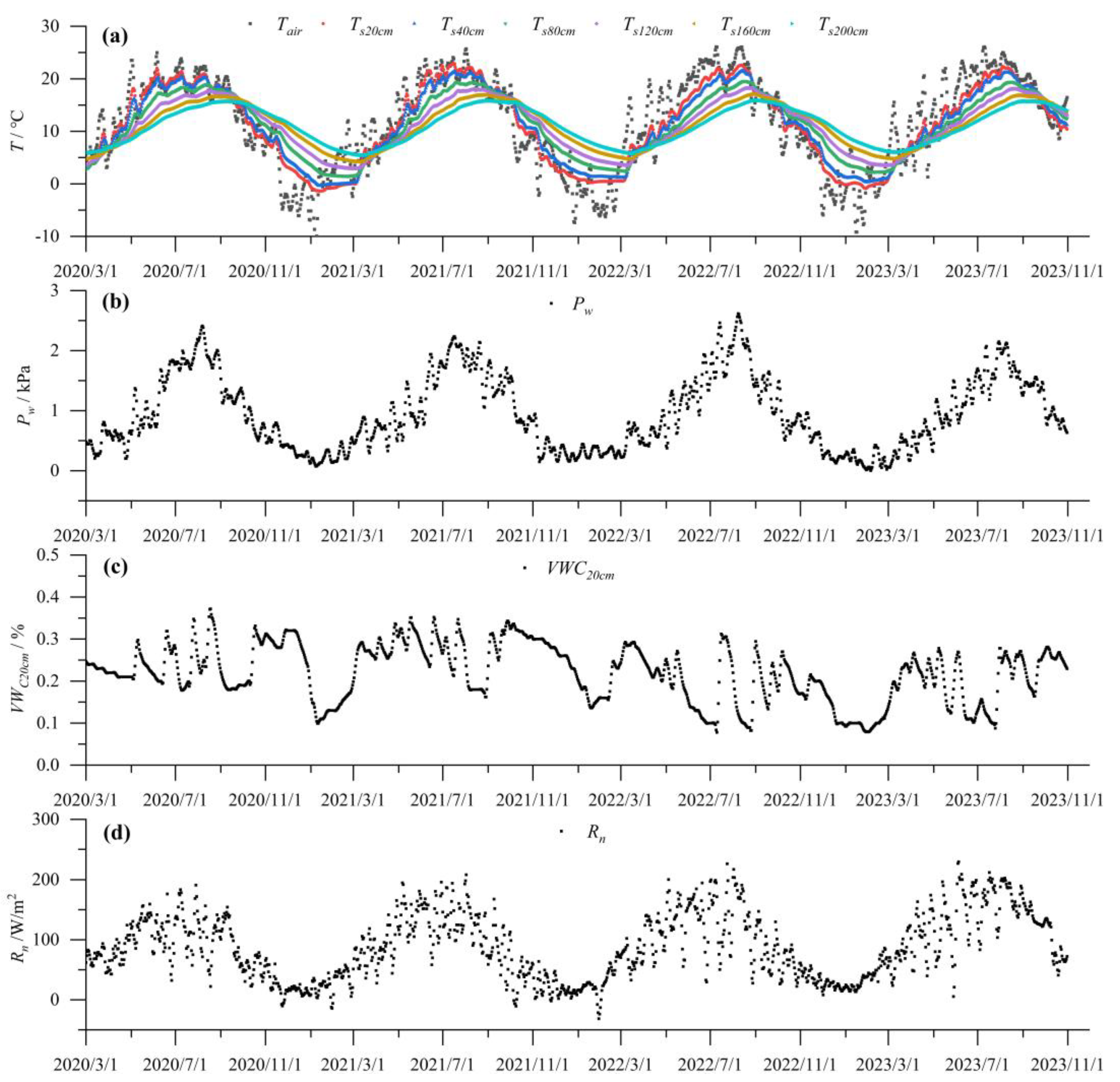
The data used in this study were all measured at the Chunhua Ecohydrology Experimental Station, and the dataset is named as Chunhua Ecohydrology Experimental Station Dataset (CEESD) including the daily soil temperatures at different depths (Ts20cm, Ts40cm, Ts80cm, Ts120cm, Ts160cm, Ts200cm), daily soil moisture at 20 cm depth (VWC20cm), daily air temperature at a height of 2 m (Tair), daily water vapor pressure (Pw), and daily net radiation (Rn). The data used in this study were measured from 1 March 2020 to 30 October 2023. There are 1340 valid daily data. For outliers and missing values in the measured data, linear interpolation was used for processing. After that, SG filter was applied to the data, and the processed data are shown in Figure 2.
As shown in Figure 2a,b,d, the daily changes in temperature, daily water vapor pressure, and daily net radiation are very drastic. But both of soil temperature at different depths, air temperature, and net radiation all have strong seasonal patterns of change. All show high values in summer and low values in winter. During the spring and summer, shallow soil temperatures are higher than deep soil temperatures. In the autumn and winter, deep soil temperatures were higher than shallow soil temperatures. Figure 2c shows that the peak of VWC20cm is concentrated from May to August each year, which is the same as the time when there is more rainfall in the region. In addition, the study area receives less precipitation in winter, resulting in a decreasing trend in VWC20cm during winter.
In general, the selection of input variables should be based on a simple relationship to achieve high accuracy in the simulation. The Pearson’s correlation coefficients among the variables (Table 1) indicated a high correlation between soil temperature and the soil temperature in the adjacent layers. The air temperature and water vapor pressure had the highest correlation with soil temperature, followed by net radiation. All of them are very suitable as input variables for soil temperature simulation. Although the linear correlation between soil moisture and soil temperature is low, soil moisture can affect temperature by controlling evaporation from the soil surface. Dry soils will reduce evaporation and thus increase surface temperatures. Conversely, wet soils usually make surface temperatures cooler [38]. Therefore, soil moisture is important for simulating shallow soil temperature, and it is also used as one of the input variables for simulating soil temperature at a depth of 20 cm (Ts20cm).
To analyze the statistical information of the selected measured data, the mean (xmean), maximum (xmax), minimum (xmin), standard deviation (xstd), variation coefficient (Cv), skewness (CS), and kurtosis (Ck) of each data series were calculated in this study. The results in Table 2 show that the maximum and minimum soil temperatures at different depths varied considerably, but the mean values of the soil temperatures at different depths did not differ much from those of the air temperatures, as soil temperatures are mainly influenced by air temperatures [26]. Both the air and soil temperatures at different depths were negatively skewed. Still, the degree of skewness of soil temperature became closer to a normal distribution as the depth of soil increased. Compared with shallow soils, deeper soil temperatures were less susceptible to strong influences from soil surface temperatures and seasonal fluctuations in temperature [39]. The results of xstd, Cv, and Cs also show that deeper soil temperatures were more stable and less volatile.
The first 80% of the data were used as the training set for training the model, and the last 20% were used as the set for testing the model. Since the observational data showed large variations, all variables used in the model were first normalized as follows:
x n o r m a l = x x m e a n x s t d
where xnormal is the normalized series of the variables, x is the original series of the observed variables, xmean is the mean of the series of the corresponding variable and xstd is the standard deviation of the series of the corresponding variable.

2.3. Methods

2.3.1. Principles of RF

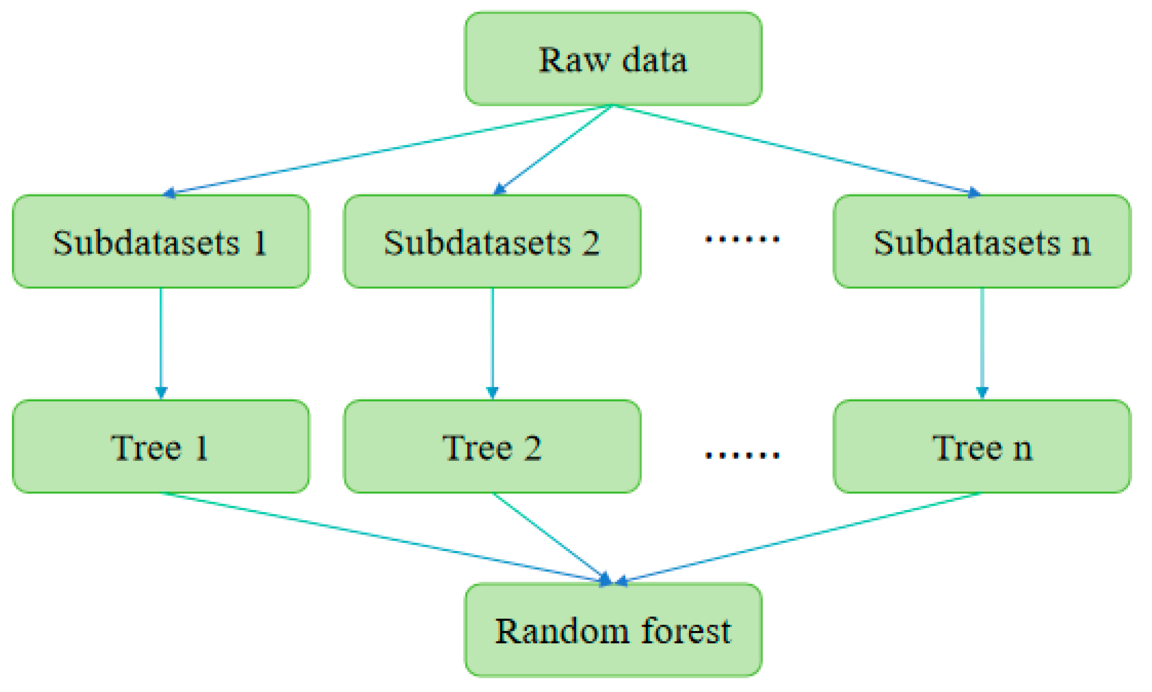
Random forest (RF) is a machine learning algorithm proposed by Breiman in 2001 based on methods such as classification, regression trees, and random subspaces [40,41]. Random forest is composed of multiple decision trees, where each regression tree is trained on a subset of data and a subset of explanatory variables that together determine the predicted values [42]. The construction process of random forest is shown in Figure 3. Random forest can effectively reduce the risk of overfitting due to its high stability and feature robustness [43]. It is now widely used in stochastic classification and stochastic regression.

2.3.2. Principles of MLP

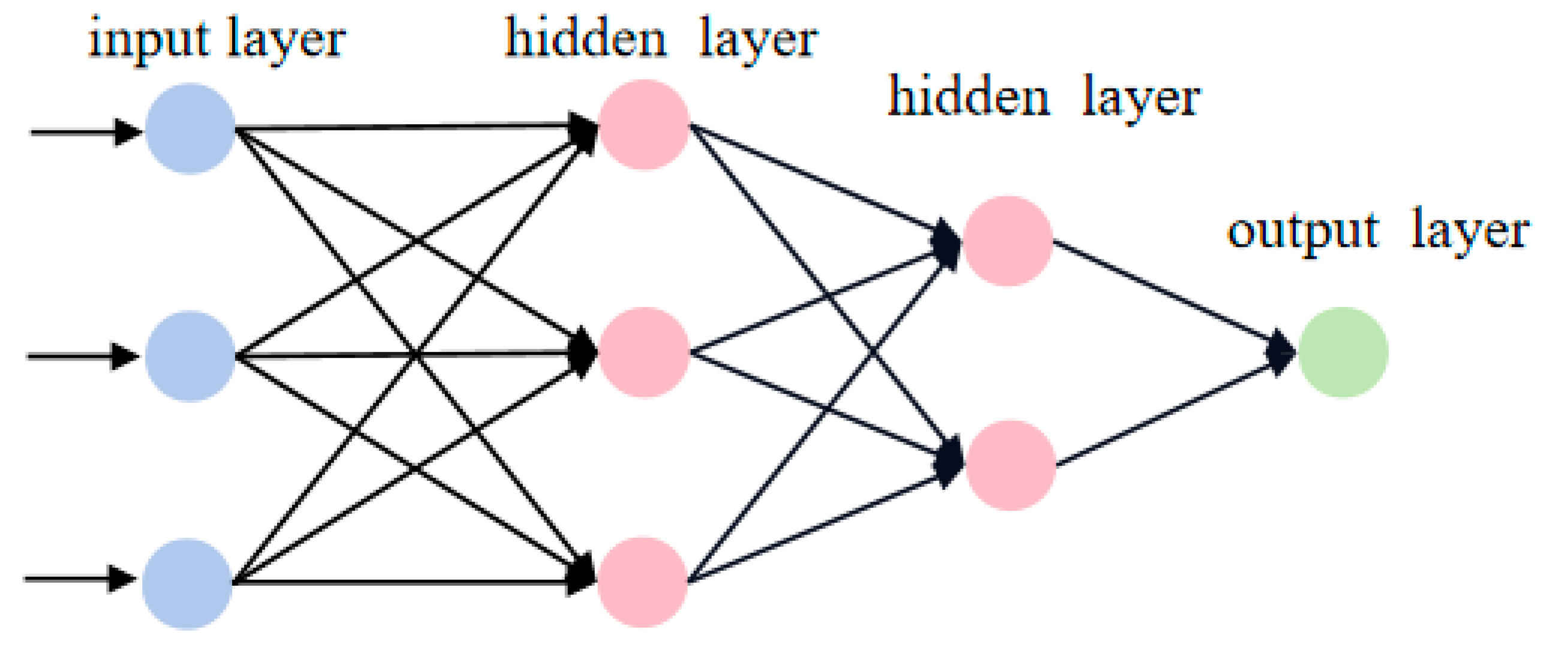
Perceptron was first proposed by Frank to solve the classification problem [40]. Multilayer perceptrons (MLP) are formed by connecting several perceptrons. MLP is a multilayer artificial neural network that can handle nonlinear relationships [44]. MLP is a forward feedback artificial neural network with good nonlinear global effect and high parallel ability. It can be used to solve classification and regression problems, and its basic structure is composed of input layer, hidden layer, and output layer [45,46], as shown in Figure 4.

2.3.3. Principles of LSTM

LSTM is widely used in simulation [47] and was first proposed by Hochreiter and Schmidhuber [48]. It is a good solution to the problems of insufficient long-term memory capacity, gradient explosion, and gradient vanishing that exist in traditional RNN [49]. It solves these problems by setting up forgetting gates, input gates, and output gates [50]. Its conventional unit structure is shown in Figure 5.
Its operation process can be expressed as follows:
i t = σ ( W h i h t 1 + W x i x t + W c i x t 1 + b i ) f t = σ ( W h f h t 1 + W x f x t + W c f x t 1 + b f ) c t = f c t 1 + i t t a n h ( W h c h t 1 + W x c x t + b i ) o t = σ ( W h o h t 1 + W x o x t + W c o x t + b 0 ) h t = o t t a n h ( c t ) y t = W h y h t + b 0
where xt and yt are the inputs and outputs of LSTM at moment t; it, ft, ct and ot are the input gates, forgetting gates, memory cell states, and output gates, respectively, at moment t; w and b are, respectively, the weight coefficient matrices and bias terms for the corresponding moments and corresponding gates; ht is the recursive input at moment t; σ is the sigmoid activation function and tanh is the hyperbolic tangent activation function.

2.3.4. Schematic Workflow of Deep Soil Temperature Prediction

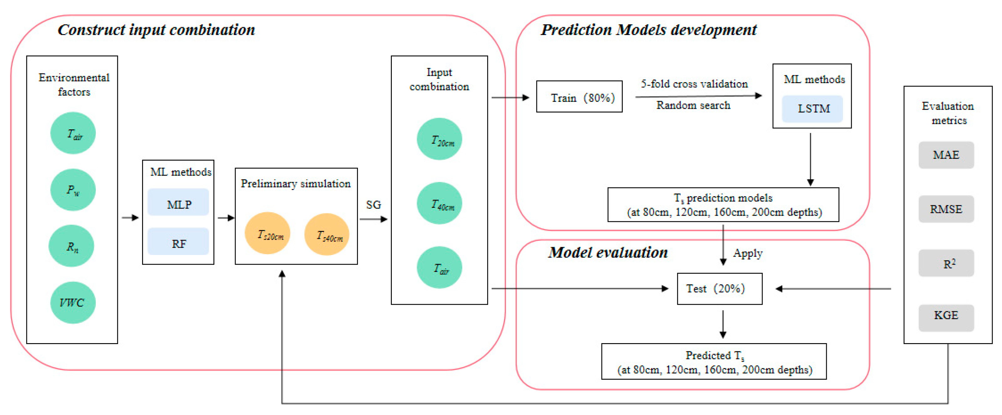
Figure 6 shows the schematic workflow of the methodology used in this study. The workflow consists of three main components: constructing input portfolios, model development, and model evaluation.
In constructing the input combination, pre-processed air temperature data (Tair), water vapor pressure data (Pw), net radiation (Rn), and soil moisture data (VWC20cm) are used as inputs for preliminary simulation of soil temperature at 20 cm depth (Ts20cm) and 40 cm depth (Ts40cm). In this section, both MLP and RF are used to simulate Ts20cm and Ts40cm. A model with better performance (evaluation metrics with better results on the test set) will be selected. After that, the simulated Ts20cm, Ts40cm, and Tair (preprocessed by SG filter) were used as the input combination to simulate soil temperature at other depths (Ts80cm, Ts120cm, Ts160cm, Ts200cm). In the model development, the first 80% of the input data were used as the training set for training the model. Five-fold cross-validation is used on the training dataset for performance evaluation of the model parameters. Random search is used to find optimal hyperparameters. The built model can predict the soil temperature of the target layer in the previous seven days based on the soil temperature and air temperature. In the model evaluation, each model predicts the concentration of Ts from the held-out testing dataset (last 20%), which was separated in the beginning and is only used for validation. The performance differences of LSTM in simulating deep soil temperature using simulated shallow soil temperature (Ts20cm, Ts40cm) and observed environmental factors (Tair, Pw) are mainly evaluated.

2.3.5. Evaluation Metrics

In this study, mean absolute error (MAE), root mean square error (RMSE), coefficient of determination (R2), and Kling–Gupta efficiency coefficient (KGE) were chosen to evaluate the results of the simulation. The formulas for calculating these are as follows:
MAE = 1 N y i y s i N RMSE = 1 N y i y s i 2 N R 2 = 1 1 N y i y s i 2 1 N y i y m 2 KGE = 1 r 1 2 + μ s μ 0 1 2 + σ s / μ s σ 0 / μ 0 1 2
where ysi and yi are the simulated values and measured values, ym is the mean of the series of measured values, N is the number of samples, μs and μ0 are the mean square deviation of the simulated values and the series of measured values, σs and σ0 are mean square deviation of the simulated value and the series of measured values, and r is the linear correlation coefficient between the simulated values and the series of measured values. Among the four model evaluation metrics, a smaller MAE and RMSE mean better performance, while when R2 and KGE are closer to 1, the result of the simulation is better.

3. Results

3.1. Input Combination of Shallow Soil Temperature

The daily air temperature (Tair), daily water vapor pressure data (Pw), net radiation (Rn), and soil moisture data (VWC20cm) were selected as input variables in this study. On the basis of the results of the correlation analysis (Table 2), four different input combinations were set up (Table 3). The correlation between air temperature, water vapor pressure, and shallow soil temperature is high. Therefore, the air temperature is used as combination 1, and the combination of air temperature and water vapor pressure is used as combination 2. Then, other variables are added to become combination 3 and combination 4.
The input combinations in Table 3 were used as input data in the RF and MLP to simulate the daily soil temperature at different depths (20 cm, 40 cm) and determine the optimal combination of input. In this preliminary simulation process, the first 80% of the data was selected for training the model, and the last 20% of the data was used for testing. Five-fold cross-validation is used on the training dataset for evaluation of the model parameters. Random search is used to find optimal hyperparameters.

3.2. Evaluation of the Results of Different Combinations of Input

The evaluation metrics of RF and MLP for simulating shallow soil temperature with different combinations of input are shown in Table 4. Both the training dataset and testing dataset reported acceptable and close results to each other according to the following: the minimum value of R2 was 0.81, the minimum value of KGE was 0.88 for the training dataset, also, the minimum value of R2 was 0.75, the minimum value of KGE was 0.80 for the testing dataset. The range of results showed a reasonable accuracy for shallow soil temperature simulation. According to the results of the evaluation metrics of different input combinations, the worst evaluation metrics of RF and MLP appear in the simulation with input combination 1, and the best evaluation metrics mostly appear in the simulation with input combination 4. The addition of meteorological factors improved the model’s performance further, and the evaluation metrics of the simulation mostly improved. The addition of meteorological factors improved the model’s performance further, and the evaluation metrics mostly improved. In the simulation of soil temperature at 40 cm depth by MLP, the MAE of input 4 is 1.1 °C lower than that of input 1, and the RMSE of input 4 is 1.47 °C lower than that of input 1. Overall, the results of the training dataset and the testing dataset all showed that input 4 produced the best simulation of the daily average temperature of the soil at different depths, so it was used as the optimal combination of the input and can be a more accurate simulation to the shallow soil temperature for the simulation of deep soil temperature.
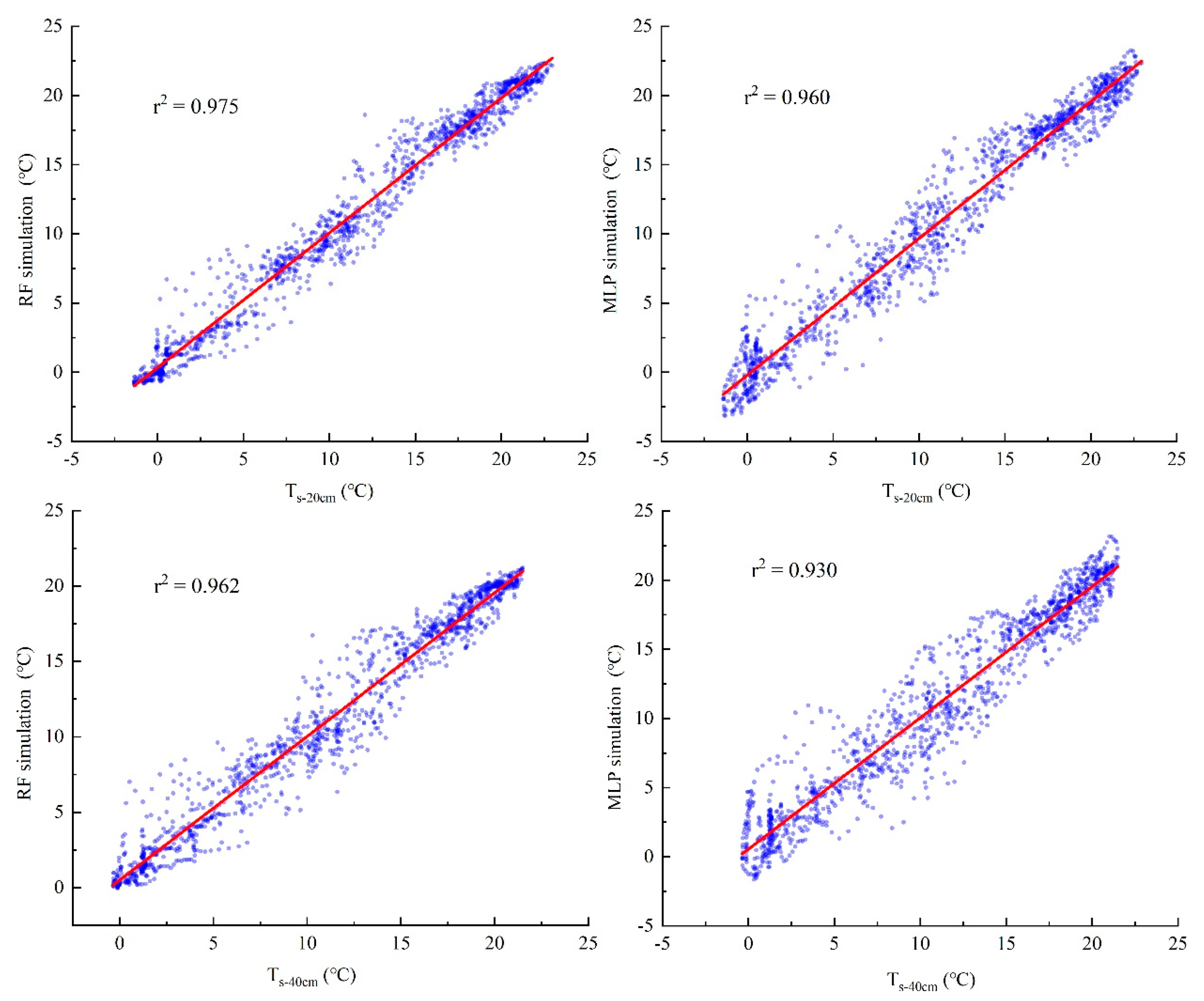
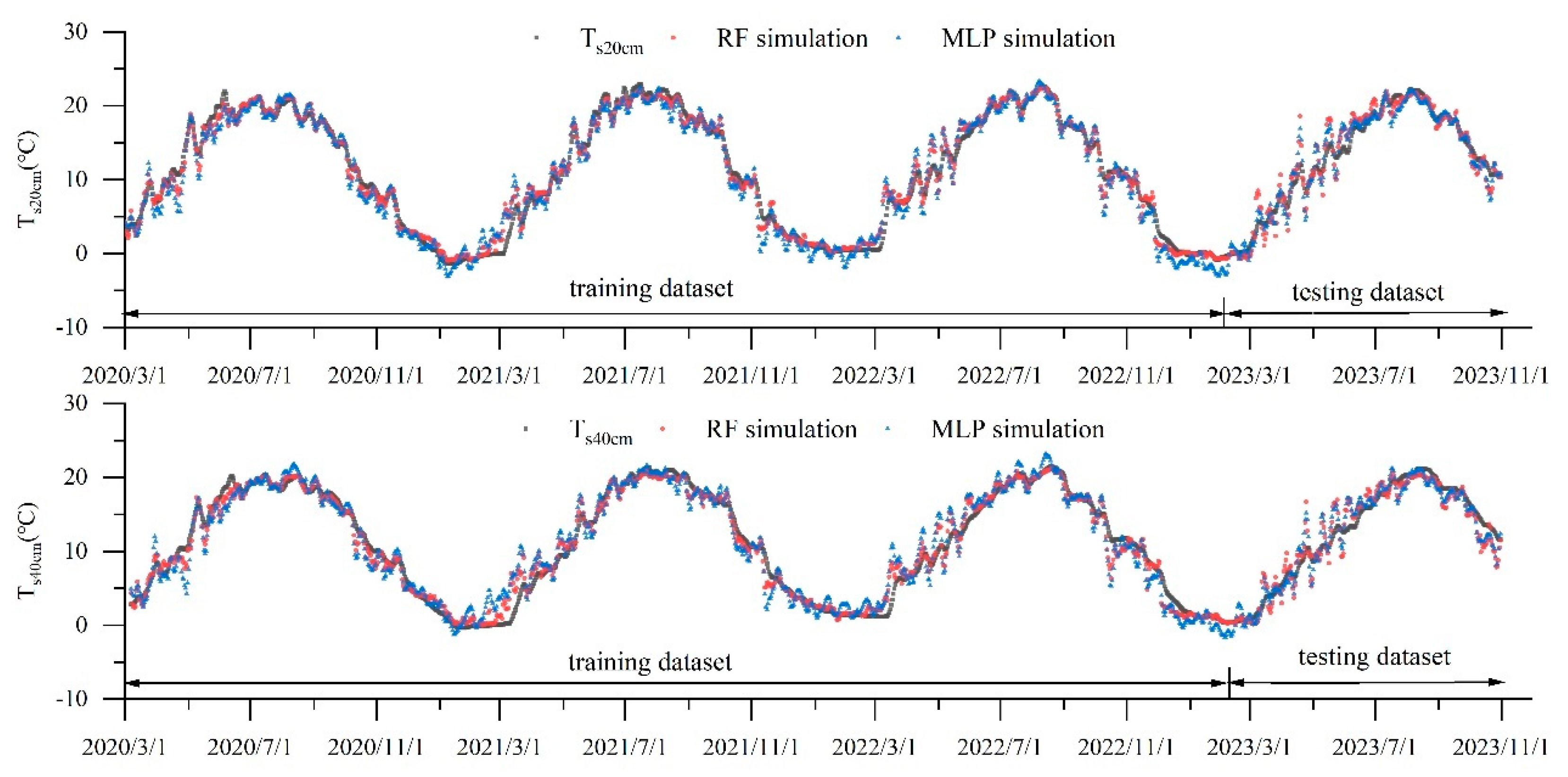
According to the scatterplots of the results from the models’ simulations versus the measured values, as shown in Figure 7, the two models simulated the soil temperature well at shallow depths (R2 was close to 1), and the accuracy of the simulations was high. Figure 8 is the time series of soil temperature measured and simulated soil temperature by RM and MLP models during the study period. It also shows an acceptable soil temperature simulated by RF and MLP however, simulating the steady change in soil temperature is a challenging task for them. The main reason is that the change in the air temperature and water vapor pressure in the input combination is very severe, while the change in soil temperature is relatively gentle. Even the air temperature after SG filtering changes much more violently than the soil temperature. It is worth noting that the simulation performance of RF on soil temperature in winter is better than that of MLP, which can simulate the steady change in soil temperature in winter. This is also the main reason why the r2 of RF is better than MLP. Figure 8 is the time series of soil temperature measured and predicted by the RF and MLP model during the study period (with the optimal combination of input). As a whole, the trend in soil temperature can be better simulated, however, the two methods have a certain underestimation of soil temperature in October.

3.3. Evaluating the Performance of LSTM Prediction of Deep Soil Temperature

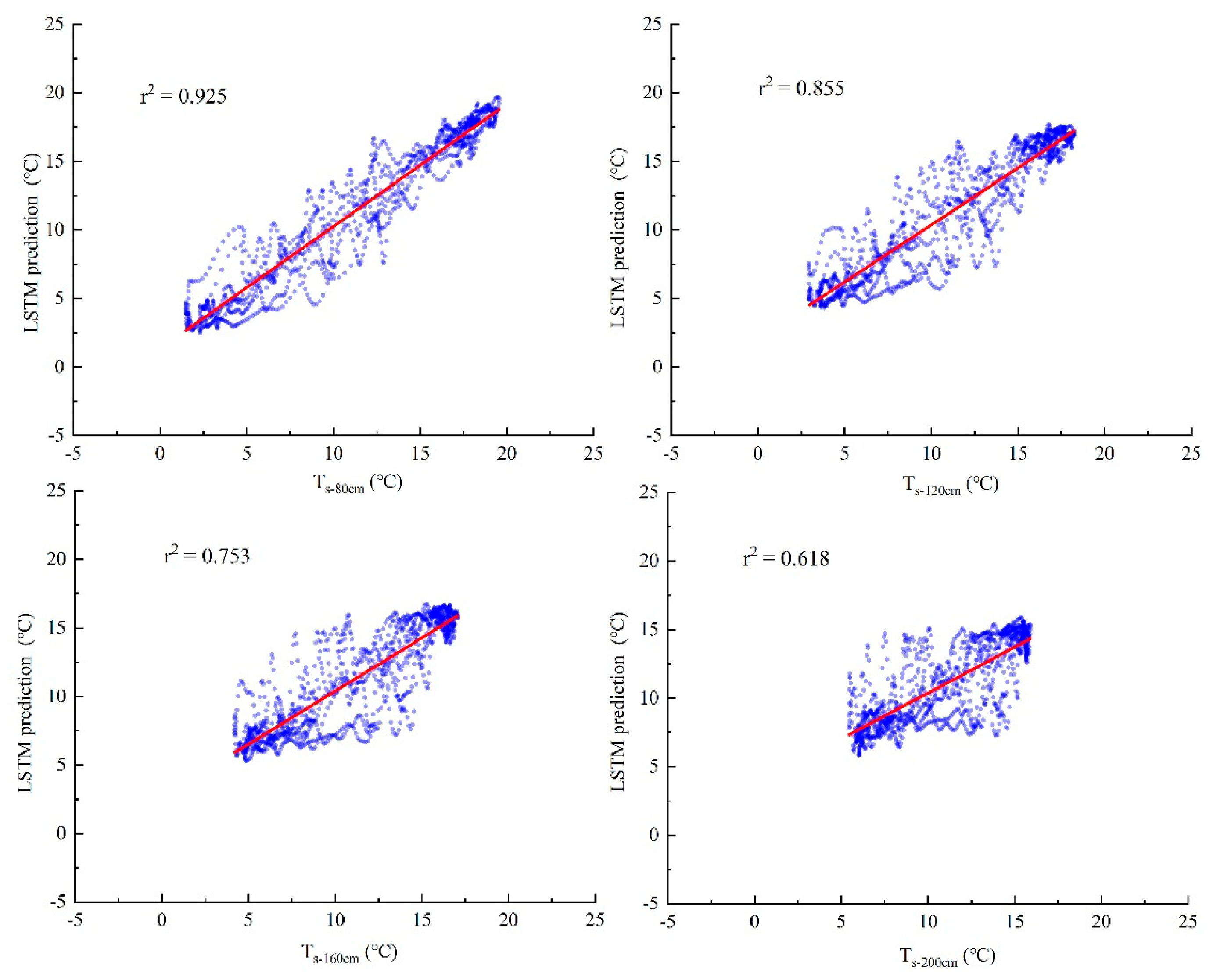
The simulated shallow soil temperature (Ts20cm, Ts40cm) and air temperature (Tair) will be used for deep soil temperature (Ts80cm, Ts120cm, Ts160cm, Ts200cm) prediction. In the model development, five-fold cross-validation is used on the training dataset for evaluation of the model parameters, and random search is used to find optimal hyperparameters. Figure 9 shows scatterplots of measured and predicted deep soil temperatures (LSTM). Their linear correlation of r2 decreases with increasing soil depth, with a maximum value of 0.928 and a minimum value of 0.625. With the increase in soil depth, the prediction error increases gradually.
Table 5 displays the evaluation metrics results. The MAE and RMSE metrics among the four evaluated metrics increased when soil depth increased, whereas R2 and KGE decreased. Both results of the training dataset and testing dataset were reported to be acceptable according to the following: the minimum value of R2 was 0.60, the minimum value of KGE was 0.74 for the training dataset, also, the minimum value of R2 was 0.66, the minimum value of KGE was 0.71 for the testing dataset. The range of results showed a reasonable accuracy for deep soil temperature prediction.
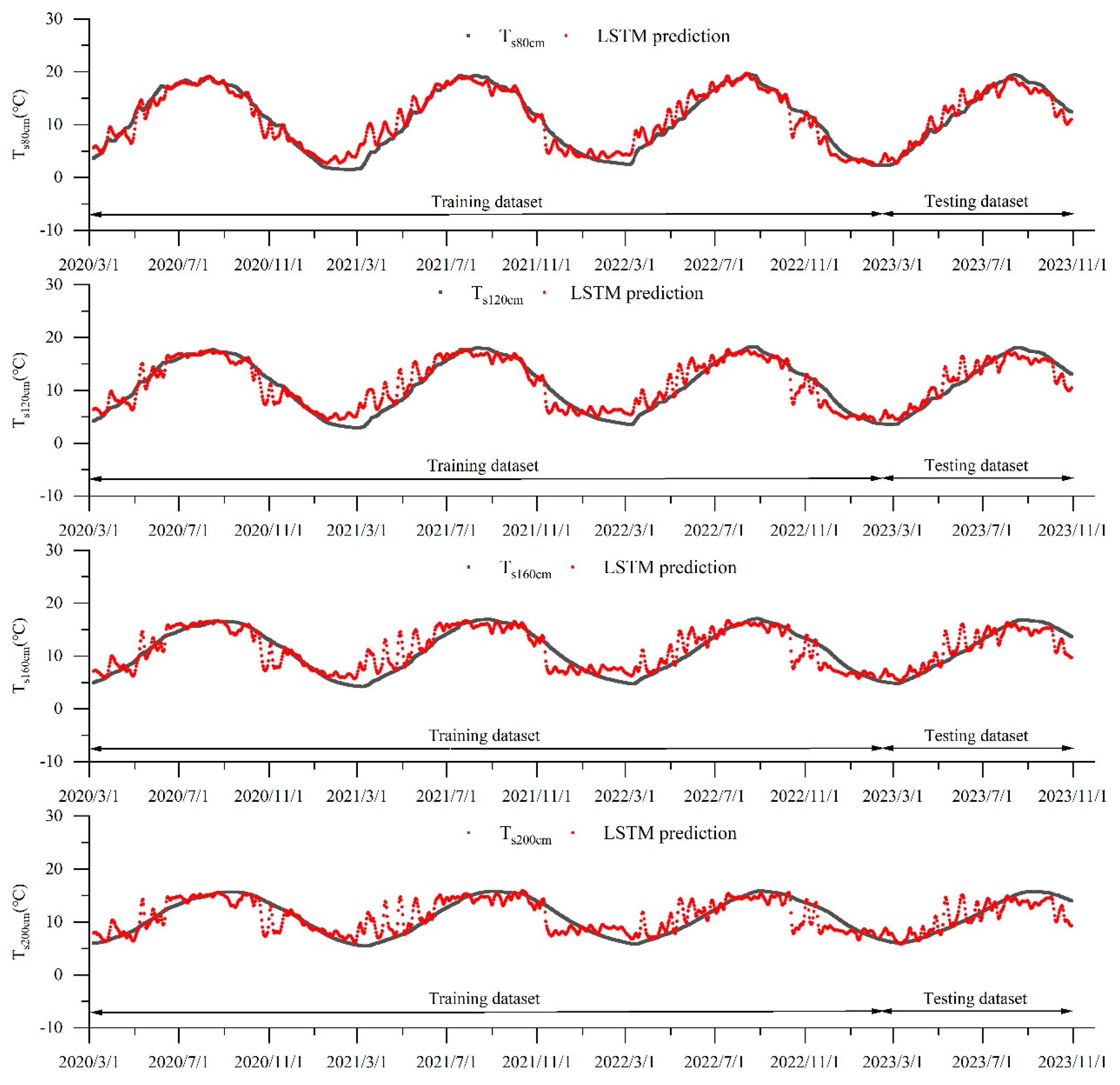
The time series of the soil temperature observed and the predicted soil temperature using the LSTM model during the study period are shown in Figure 10. As a whole, the trend in soil temperature can be better predicted after using the shallow soil temperature and air temperature from seven days prior. It also shows that the LSTM model simulates high and low temperatures more accurately and that the simulation error-prone places are distributed close to the temperature change. The soil temperature is higher in summer and lower in winter. One of the primary reasons the soil temperature predicted is more precise and constant is that the summertime temperature is a continuous hot temperature, and the wintertime temperature is also a continuous low temperature.
The air temperature, water vapor pressure, net radiation, and soil moisture can also be directly used to predict deep soil temperature. The evaluation metrics are shown in Table 6 (prediction using environmental factors from seven days ago). In the testing dataset, the prediction results are worse than the prediction method proposed in this study, especially at 200 cm, where r2 is only 0.579.

3.4. Impact of Sliding Panes on Prediction Accuracy

The LSTM model was used to predict deep soil temperature. In this study, shallow soil temperatures are the important input variables for prediction, and their simulation accuracy certainly has an impact on the prediction accuracy. Not only do the input variables have an effect on the prediction accuracy, but the length of the data used for prediction (the size of the sliding panes) also has an effect on the prediction accuracy. The sliding panes refer to dividing the time series data into continuous windows during the training process and using these panes to train the model. In this section, setting different sizes of the sliding panes are used for prediction and their performance differences are compared. The different sizes of the sliding panes are shown in Table 7.
The prediction results of the different models in Table 7 are shown in Table 8. The results show that all evaluation metrics become better with the increase in the size of the sliding panes. It was also found that the size of the sliding pane was directly related to the magnitude of the fluctuations in the predicted values. The larger the size of the sliding pane, the smoother the predicted values. This suggests that when the size of the sliding panes is too small, the model is likely to fail to capture long-term data features. Thus, choosing the right sliding window size is equally important. The optimal sliding pane size is often achieved through continuous experimentation.

3.5. Effect of Savitzky–Golay Filter on Prediction Accuracy

The Savitzky–Golay filter is commonly used in data preprocessing processes to eliminate data noise and reduce data fluctuations. Compared to simple moving average filtering, SG filter can better retain the overall trend of the data while smoothing it. SG filter is also used in this study for post-processing the prediction data of the LSTM7 model (projections using data from the previous seven days) to explore whether it can further improve prediction accuracy. The postprocessed model is named LSTM7-SG. The results of the evaluation indicators are shown in Table 9. It shows that SG filter postprocessing of LSTM7 can improve the results of some evaluation metrics, but the improvement is very limited. This also suggests that the SG filter is more suitable for data preprocessing.

4. Discussion

From the perspective of energy exchange, heat transfer occurs between the temperature of the air and the soil, and the air temperature greatly affects the soil temperature [51]. The change in soil moisture can control the partitioning of surface energy between sensible and latent heat fluxes through evapotranspiration, and they jointly drive the change in soil temperature [52,53,54]. Shallow soil temperature plays a significant role in the land–air heat exchange that determines the underground temperature of deep soil [55]. This shows that both air temperature and soil moisture have the potential to simulate soil temperature, and shallow soil temperature also has the potential to simulate deep soil temperature. Currently, a number of researchers have found that air temperature, solar radiation, and rainfall in combination may accurately simulate the soil temperature of different areas that have different climatic and geographical circumstances [7,25,56,57]. In our research, air temperature, water vapor pressure, net radiation, and soil moisture were used to simulate soil temperature. Air temperature has a direct impact on soil temperature. The magnitude of water vapor pressure depends on the amount of water vapor in the atmosphere [58]. Soil moisture directly indicates the condition of water content in the soil. The difference between downward and upward (sun and earth) radiation is referred to as net radiation [59]. To an extent, soil moisture and water vapor pressure can reflect the amount of rainfall. In contrast to solar radiation, net radiation takes into account the impact of upward radiation on the Earth. The selection of input variables is an essential task in time series prediction, and the choice of variables is dependent on the quality and correlation of the data. Rainfall has a far lower correlation with shallow soil temperature than water vapor pressure and soil moisture. Based on the findings of previous research, this is a new attempt to simulate soil temperature using several factors, which may potentially have broader applicability. However, the experimental site is only Chunhua Experimental Station in the Hejiashan watershed, its applicability in other regions still needs to be verified.
For the machine learning methods used in this study, RF may reduce the danger of overfitting for the machine learning methods utilized in this work [60]. MLP is quite good at modeling nonlinearities [23]. Both of them are more skilled at using a wide range of environmental inputs to determine the temperature of the shallow soil and improve the simulation’s impact. Furthermore, neither of the two models will lose data and their simulation speeds are quicker than LSTM. Therefore, to simulate the shallow soil temperature, RF and MLP have been used. Long-term dependencies in sequence data may be efficiently captured by LSTM, which can also thoroughly mine the link between input data and target variables. It is excellent for forecasting [55].
Accurately estimating soil temperature is critical to carry out agricultural planting activities. To a certain extent, the planting time of field crops and greenhouse crops all depends on the optimal soil temperature for seed germination and seedling emergence [34,61]. Different crops demand different temperatures for optimal growth. In order to help farmers better plan when to sow their crops, this study proposes a model that can accurately predict soil temperature. This could improve the crop’s survival rate, which will raise output and boost farmers’ income. In addition, the exploration of input combinations can also identify the number of environmental factors, so as to select the most suitable number of equipment to monitor research areas and reduce the cost of site equipment.

5. Conclusions

With on-site observation data, including the measured temperature of the soil and different environmental factors, RF and MLP are used to simulate shallow soil temperature, and LSTM is used to predict deep soil temperature in the gully areas of the Loess Plateau in China. The main conclusions are as follows:
(1)
For different combinations of input variables, the inclusion of relevant environmental factors can improve the model’s performance. When the daily temperature of the air is at a height of 2 m (Tair), daily water vapor pressure data (Pw), net radiation (Rn), and soil moisture data (VWC20cm) were jointly used as inputs for all the simulations at 20 cm and 40 cm depths, the results of RF and MLP were the best. Both RF and MLP can simulate shallow soil temperature well, but the performance of MLP is better than that of RF.
(2)
It is feasible to use LSTM to predict the deep soil temperature with the simulated shallow soil temperature and the measured air temperature as input.
(3)
The accuracy of soil temperature prediction is different at different depths. With the increase in soil depth, the accuracy of soil temperature prediction decreases. The simulation accuracy of shallow soil temperature directly affects the prediction accuracy of deep soil temperature. In addition, the size of the sliding pane of the LSTM model also affects the prediction accuracy.
(4)
The SG filter is more suitable for data preprocessing, and its ability to post-process prediction results is very limited.
This study evaluated the feasibility of simulating the daily soil temperature using conventional machine learning techniques (MLR and MLP) for shallow soil temperature. The combination of input variables in the shallow soil simulation was mostly determined by the variables’ physical relevance and by doing numerous experiments. More attention could be paid to the interrelationships among the environmental factors and other environmental factors in future studies to further improve the stability and accuracy of the simulation. LSTM is used to predict deep soil temperature. In the process of prediction, due to the small amount of data, the predicted soil temperature still has some instability. In addition, the design of the sliding pane size of the prediction model also only depends on repeated experiments. In the future, we can focus on optimizing the setting of the window size and the setting of the input combination.

Author Contributions

Conceptualization, D.L.; methodology, D.L. and W.D.; software, W.D. and L.M.; validation, F.G.; formal analysis, W.D.; investigation, D.L., W.D., F.G., L.Z. and L.M.; resources, D.L. and Q.H.; data curation, D.L., W.D., F.G. and L.Z.; writing—original draft preparation, W.D.; writing—review and editing, D.L., Q.L., G.M., F.G., L.M. and X.M.; visualization, W.D. and L.M.; supervision, Q.H.; project administration, D.L.; funding acquisition, D.L. All authors have read and agreed to the published version of the manuscript.

Funding

This research was supported by the National Natural Science Foundation of China (NSFC) (Grant Nos. 52279025, 42071335, and 52109031) and the National Key Research and Development Program of China (2022YFF1302200).

Data Availability Statement

The experimental data used in this study were obtained from the Chunhua Ecohydrology Experimental Station of Xi’an University of Technology and the dataset is named Chunhua Ecohydrology Experimental Station Dataset (CEESD), which can be obtained from the corresponding author (Dengfeng Liu, [email protected]) upon personal reasonable request.

Conflicts of Interest

Author Guanghui Ming was employed by the company Yellow River Engineering Consulting Co., Ltd. The remaining authors declare that the research was conducted in the absence of any commercial or financial relationships that could be construed as a potential conflict of interest.

References

  1. Veldhuizen, L.J.; Giller, K.E.; Oosterveer, P.; Brouwer, I.D.; Janssen, S.; van Zanten, H.H.; Slingerland, M.A. The Missing Middle: Connected action on agriculture and nutrition across global, national and local levels to achieve Sustainable Development Goal 2. Glob. Food Secur. 2020, 24, 100336. [Google Scholar] [CrossRef]
  2. Linghu, L.; Sun, P.; Zhang, M.; Wu, Y. Data-Driven Projections Demonstrate Non-Farming Use of Cropland in Non-Major Grain-Producing Areas: A Case Study of Shaanxi Province, China. Agronomy 2023, 13, 2060. [Google Scholar] [CrossRef]
  3. Furtak, K.; Gawryjołek, K.; Marzec-Grządziel, A.; Niedźwiecki, J. The Influence of Human Agricultural Activities on the Quality of Selected Fluvisols from the Vistula River Valley, Poland—Preliminary Research. Agronomy 2024, 14, 480. [Google Scholar] [CrossRef]
  4. Zeynoddin, M.; Ebtehaj, I.; Bonakdari, H. Development of a linear based stochastic model for daily soil temperature prediction: One step forward to sustainable agriculture. Comput. Electron. Agric. 2020, 176, 105636. [Google Scholar] [CrossRef]
  5. Seyfried, M.S.; Flerchinger, G.N.; Murdock, M.D.; Hanson, C.L.; Van Vactor, S. Long-Term Soil Temperature Database, Reynolds Creek Experimental Watershed, Idaho, United States. Water Resour. Res. 2001, 37, 2843–2846. [Google Scholar] [CrossRef]
  6. Kramer, P.J. Effects of Soil Temperature on the Absorption of Water by Plants. Science 1934, 79, 371–372. [Google Scholar] [CrossRef] [PubMed]
  7. Alizamir, M.; Kisi, O.; Ahmed, A.N.; Mert, C.; Fai, C.M.; Kim, S.; Kim, N.W.; El-Shafie, A.; Lin, L. Advanced machine learning model for better prediction accuracy of soil temperature at different depths. PLoS ONE 2020, 15, e231055. [Google Scholar] [CrossRef] [PubMed]
  8. Ganeshi, N.G.; Mujumdar, M.; Takaya, Y.; Goswami, M.M.; Singh, B.B.; Krishnan, R.; Terao, T. Soil moisture revamps the temperature extremes in a warming climate over India. npj Clim. Atmos. Sci. 2023, 6, 12. [Google Scholar] [CrossRef]
  9. Onwuka, B.; Mang, B. Effects of soil temperature on some soil properties and plant growth. Adv. Plants Agric. Res. 2018, 8, 34–37. [Google Scholar] [CrossRef]
  10. Yin, X.; Arp, P.A. Predicting forest soil temperatures from monthly air temperature and precipitation records. Can. J. Forest Res. 1993, 23, 2521–2536. [Google Scholar] [CrossRef]
  11. Zhao, H.; Sassenrath, G.F.; Kirkham, M.B.; Wan, N.; Lin, X. Daily soil temperature modeling improved by integrating observed snow cover and estimated soil moisture in the USA Great Plains. Hydrol. Earth Syst. Sci. 2021, 25, 4357–4372. [Google Scholar] [CrossRef]
  12. Mihalakakou, G. On estimating soil surface temperature profiles. Energy Build. 2002, 34, 251–259. [Google Scholar] [CrossRef]
  13. Qi, J.; Li, S.; Li, Q.; Xing, Z.; Bourque, P.A.; Meng, F.R. A new soil-temperature module for SWAT application in regions with seasonal snow cover. J. Hydrol. 2016, 538, 863–877. [Google Scholar] [CrossRef]
  14. Padarian, J.; Minasny, B.; McBratney, A.B. Machine learning and soil sciences: A review aided by machine learning tools. Soil 2020, 6, 35–52. [Google Scholar] [CrossRef]
  15. Recknagel, F.; French, M.; Harkonen, P.; Yabunaka, K. Artificial neural network approach for modelling and prediction of algal blooms. Ecol. Model. 1997, 96, 11–28. [Google Scholar] [CrossRef]
  16. Lin, X.; Duan, X.; Jacobs, C.; Ullmann, J.; Chan, C.; Chen, S.; Cheng, S.; Zhao, W.; Poduri, A.; Wang, X.; et al. High-throughput brain activity mapping and machine learning as a foundation for systems neuropharmacology. Nat. Commun. 2018, 9, 5142. [Google Scholar] [CrossRef] [PubMed]
  17. Hulbert, C.; Rouet-Leduc, B.; Johnson, P.A.; Ren, C.X.; Rivière, J.; Bolton, D.C.; Marone, C. Similarity of fast and slow earthquakes illuminated by machine learning. Nat. Geosci. 2019, 12, 69–74. [Google Scholar] [CrossRef]
  18. Fang, K.; Kifer, D.; Lawson, K.; Shen, C. Evaluating the potential and challenges of an uncertainty quantification method for long short-term memory models for soil moisture predictions. Water Resour. Res. 2020, 56, e2020WR028095. [Google Scholar] [CrossRef]
  19. Cui, Q.; Ammar, M.E.; Iravani, M.; Kariyeva, J.; Faramarzi, M. Regional wetland water storage changes: The influence of future climate on geographically isolated wetlands. Ecol. Indic. 2021, 120, 106941. [Google Scholar] [CrossRef]
  20. Zhong, L.; Lei, H.; Gao, B. Developing a Physics-Informed Deep Learning Model to Simulate Runoff Response to Climate Change in Alpine Catchments. Water Resour. Res. 2023, 59, e2022WR034118. [Google Scholar] [CrossRef]
  21. Nabavi-Pelesaraei, A.; Shaker-Koohi, S.; Dehpour, M.B. Modeling and optimization of energy inputs and greenhouse gas emissions for eggplant production using artificial neural network and multi-objective genetic algorithm. Int. J. Adv. Biol. Biomed. Res. 2013, 4, 170–183. [Google Scholar]
  22. Sándor, R.; Barcza, Z.; Acutis, M.; Doro, L.; Hidy, D.; Chy, M.K.; Minet, J.; Lellei-Kovács, E.; Ma, S.; Perego, A. Multi-model simulation of soil temperature, soil water content and biomass in Euro-Mediterranean grasslands: Uncertainties and ensemble performance. Eur. J. Agron. 2017, 88, 22–40. [Google Scholar] [CrossRef]
  23. Samadianfard, S.; Ghorbani, M.A.; Mohammadi, B. Forecasting soil temperature at multiple-depth with a hybrid artificial neural network model coupled-hybrid firefly optimizer algorithm. Inf. Process. Agric. 2018, 5, 465–476. [Google Scholar] [CrossRef]
  24. Li, Q.; Hao, H.; Zhao, Y.; Geng, Q.; Liu, G.; Zhang, Y.; Yu, F. GANs-LSTM Model for Soil Temperature Estimation from Meteorological: A New Approach. IEEE Access 2020, 8, 59427–59443. [Google Scholar] [CrossRef]
  25. Nahvi, B.; Habibi, J.; Mohammadi, K.; Shamshirband, S.; Al Razgan, O.S. Using self-adaptive evolutionary algorithm to improve the performance of an extreme learning machine for estimating soil temperature. Comput. Electron. Agric. 2016, 124, 150–160. [Google Scholar] [CrossRef]
  26. Bayatvarkeshi, M.; Bhagat, S.K.; Mohammadi, K.; Kisi, O.; Farahani, M.; Hasani, A.; Deo, R.; Yaseen, Z.M. Modeling soil temperature using air temperature features in diverse climatic conditions with complementary machine learning models. Comput. Electron. Agric. 2021, 185, 106158. [Google Scholar] [CrossRef]
  27. Tsai, Y.Z.; Hsu, K.S.; Wu, H.Y.; Lin, S.I.; Yu, H.L.; Huang, K.T.; Hu, M.C.; Hsu, S.Y. Application of random forest and ICON models combined with weather forecasts to predict soil temperature and water content in a greenhouse. Water 2020, 12, 1176. [Google Scholar] [CrossRef]
  28. Recknagel, F. Applications of machine learning to ecological modelling. Ecol. Model. 2001, 146, 303–310. [Google Scholar] [CrossRef]
  29. Massoud, E.C.; Hoffman, F.; Shi, Z.; Tang, J.; Alhajjar, E.; Barnes, M.; Braghiere, R.K.; Cardon, Z.; Collier, N.; Crompton, O.; et al. Perspectives on Artificial Intelligence for Predictions in Ecohydrology. Artif. Intell. Earth Syst. 2023, 2, e230005. [Google Scholar] [CrossRef]
  30. Chan, W.S.; Recknagel, F.; Cao, H.; Park, H. Elucidation and short-term forecasting of microcystin concentrations in Lake Suwa (Japan) by means of artificial neural networks and evolutionary algorithms. Water Res. 2007, 41, 2247–2255. [Google Scholar] [CrossRef]
  31. Li, C.; Zhang, Y.; Ren, X. Modeling Hourly Soil Temperature Using Deep BiLSTM Neural Network. Algorithms 2020, 13, 173. [Google Scholar] [CrossRef]
  32. Tsai, W.P.; Feng, D.; Pan, M.; Beck, H.; Lawson, K.; Yang, Y.; Liu, J.; Shen, C. From calibration to parameter learning: Harnessing the scaling effects of big data in geoscientific modeling. Nat. Commun. 2020, 12, 5988. [Google Scholar] [CrossRef]
  33. Li, X.; Zhang, L.; Wang, X.; Liang, B. Forecasting greenhouse air and soil temperatures: A multi-step time series approach employing attention-based LSTM network. Comput. Electron. Agric. 2024, 217, 108602. [Google Scholar] [CrossRef]
  34. Khosravi, K.; Golkarian, A.; Barzegar, R.; Aalami, M.T.; Heddam, S.; Omidvar, E.; Keesstra, S.D.; López-Vicente, M. Multi-step ahead soil temperature forecasting at different depths based on meteorological data: Integrating resampling algorithms and machine learning models. Pedosphere 2023, 33, 479–495. [Google Scholar] [CrossRef]
  35. Taki, M.; Abdanan Mehdizadeh, S.; Rohani, A.; Rahnama, M.; Rahmati-Joneidabad, M. Applied machine learning in greenhouse simulation; new application and analysis. Inf. Process. Agric. 2018, 5, 253–268. [Google Scholar] [CrossRef]
  36. Zhang, K.; Liu, D.; Liu, H.; Lei, H.; Guo, F.; Xie, S.; Meng, X.; Huang, Q. Energy flux observation in a shrub ecosystem of a gully region of the Chinese Loess Plateau. Ecohydrol. Hydrobiol. 2022, 22, 323–336. [Google Scholar] [CrossRef]
  37. Guo, F.; Liu, D.; Mo, S.; Huang, Q.; Ma, L.; Xie, S.; Deng, W.; Ming, G.; Fan, J. Estimation of daily evapotranspiration in gully area scrub ecosystems on Loess Plateau of China based on multisource observation data. Ecol. Indic. 2023, 154, 110671. [Google Scholar] [CrossRef]
  38. Trok, J.T.; Davenport, F.V.; Barnes, E.A.; Diffenbaugh, N.S. Using Machine Learning with Partial Dependence Analysis to Investigate Coupling Between Soil Moisture and Near-Surface Temperature. J. Geophys. Res. Atmos. 2023, 128, e2022JD038365. [Google Scholar] [CrossRef]
  39. Sahoo, M. Winter soil temperature and its effect on soil nitrate Status: A Support Vector Regression-based approach on the projected impacts. Catena 2022, 211, 105958. [Google Scholar] [CrossRef]
  40. Rosenblatt, F. The perceptron: A probabilistic model for information storage and organization in the brain. Psychol. Rev. 1958, 65, 386–408. [Google Scholar] [CrossRef]
  41. Ho, T.K. The random subspace method for constructing decision forests. IEEE Trans. Pattern Anal. Mach. Intell. 1998, 20, 832–844. [Google Scholar]
  42. Isles, P.D.F. A random forest approach to improve estimates of tributary nutrient loading. Water Res. 2024, 248, 120876. [Google Scholar] [CrossRef]
  43. Han, T.; Jiang, D.; Zhao, Q.; Wang, L.; Yin, K. Comparison of random forest, artificial neural networks and support vector machine for intelligent diagnosis of rotating machinery. Trans. Inst. Meas. Control 2017, 40, 2681–2693. [Google Scholar] [CrossRef]
  44. Mohanty, M.D.; Mohanty, M.N. Chapter 5—Verbal sentiment analysis and detection using recurrent neural network. In Advanced Data Mining Tools and Methods for Social Computing; De, S., Dey, S., Bhattacharyya, S., Bhatia, S., Eds.; Academic Press: Cambridge, MA, USA, 2022; pp. 85–106. [Google Scholar]
  45. Abirami, S.; Chitra, P. Chapter Fourteen—Energy-efficient edge based real-time healthcare support system. In Advances in Computers; Raj, P., Evangeline, P., Eds.; Elsevier: Amsterdam, The Netherlands, 2020; Volume 117, pp. 339–368. [Google Scholar]
  46. Abinaya, S.; Devi, M.K.K. Chapter 12—Enhancing crop productivity through autoencoder-based disease detection and context-aware remedy recommendation system. In Application of Machine Learning in Agriculture; Khan, M.A., Khan, R., Ansari, M.A., Eds.; Academic Press: Cambridge, MA, USA, 2022; pp. 239–262. [Google Scholar]
  47. Rahmani, F.; Shen, C.; Oliver, S.; Lawson, K.; Appling, A. Deep learning approaches for improving prediction of daily stream temperature in data-scarce, unmonitored, and dammed basins. Hydrol. Process. 2021, 35, e14400. [Google Scholar] [CrossRef]
  48. Hochreiter, S.; Schmidhuber, J. Long Short-Term Memory. Neural Comput. 1997, 9, 1735–1780. [Google Scholar] [CrossRef]
  49. Huang, S.; Liu, Q.; Wu, Y.; Chen, M.; Yin, H.; Zhao, J. Edible Mushroom Greenhouse Environment Prediction Model Based on Attention CNN-LSTM. Agronomy 2024, 14, 473. [Google Scholar] [CrossRef]
  50. Di, Y.; Gao, M.; Feng, F.; Li, Q.; Zhang, H. A New Framework for Winter Wheat Yield Prediction Integrating Deep Learning and Bayesian Optimization. Agronomy 2022, 12, 3194. [Google Scholar] [CrossRef]
  51. Bai, Y.; Scott, T.A.; Min, Q. Climate change implications of soil temperature in the Mojave Desert, USA. Front. Earth Sci. 2014, 8, 302–308. [Google Scholar] [CrossRef]
  52. Miralles, D.G.; Van, D.B.M.J.; Teuling, A.J.; De Jeu, R.A.M. Soil moisture-temperature coupling: A multiscale observational analysis. Geophys. Res. Lett. 2012, 39, 6. [Google Scholar] [CrossRef]
  53. Zhang, T.; Huang, J.; Lei, Q.; Liang, X.; Lindsey, S.; Luo, J.; Zhu, A.; Bao, W.; Liu, H. Empirical estimation of soil temperature and its controlling factors in Australia: Implication for interaction between geographic setting and air temperature. Catena 2022, 208, 105696. [Google Scholar] [CrossRef]
  54. Xu, Y.; Wang, P.; Lu, Y.; Ma, M.; Dong, G.; Tang, J. Convection-permitting regional climate simulation on soil moisture-heatwaves relationship over eastern China. Atmos. Res. 2024, 301, 107285. [Google Scholar] [CrossRef]
  55. Amato, M.T.; Giménez, D. Predicting monthly near-surface soil temperature from air temperature and the leaf area index. Agric. Forest Meteorol. 2024, 345, 109838. [Google Scholar] [CrossRef]
  56. Citakoglu, H. Comparison of artificial intelligence techniques for prediction of soil temperatures in Turkey. Theor. Appl. Climatol. 2017, 130, 545–556. [Google Scholar] [CrossRef]
  57. Gao, S.; Wu, Q.; Zhang, Z.; Jiang, G. Simulating active layer temperature based on weather factors on the Qinghai–Tibetan Plateau using ANN and wavelet-ANN models. Cold Reg. Sci. Technol. 2020, 177, 103118. [Google Scholar] [CrossRef]
  58. Gao, B.; Coon, E.T.; Thornton, P.E.; Lu, D. Improving the estimation of atmospheric water vapor pressure using interpretable long short-term memory networks. Agric. Forest Meteorol. 2024, 347, 109907. [Google Scholar] [CrossRef]
  59. Bonachela, S.; Fernández, M.D.; Hernández, J.; López, J.C. Adaptation of standardised (FAO and ASCE) procedures of estimating net longwave and shortwave radiation to Mediterranean greenhouse crops. Biosyst. Eng. 2023, 231, 104–116. [Google Scholar] [CrossRef]
  60. He, Z.; Wang, J.; Jiang, M.; Hu, L.; Zou, Q. Random Subsequence Forests. Inf. Sci. 2024, 667, 120478. [Google Scholar] [CrossRef]
  61. Jiao, Y.; Chen, C.; Li, G.; Fu, H.; Mi, X. Research on the variation patterns and predictive models of soil temperature in a solar greenhouse. Sol. Energy 2024, 270, 112267. [Google Scholar] [CrossRef]
Figure 1. The location of the experimental station and the observation system. (a) DEM of Shaanxi Province and the location of Chunhua Ecohydrology Experimental Station. (b) Meteorological observation tower and equipment at the station.
Agronomy 14 00703 g001
Figure 2. Time series of data. (a) The daily soil temperatures at different depths and daily air temperature at a height of 2 m. (b) The daily water vapor pressure. (c) The daily soil moisture at 20 cm depth. (d) The daily net radiation.
Agronomy 14 00703 g002
Figure 3. Structure of RF.
Agronomy 14 00703 g003
Figure 4. Structure of MLP.
Agronomy 14 00703 g004
Figure 5. Unit structure of LSTM.
Agronomy 14 00703 g005
Figure 6. Schematic workflow of this study. (RF, MLP, and LSTM are different machine learning models. RF = random forest, MLP = multilayer perceptron, LSTM = long short-term memory).
Agronomy 14 00703 g006
Figure 7. Scatterplots of the simulated and measured shallow soil temperatures.
Agronomy 14 00703 g007
Figure 8. Simulated and measured shallow soil temperatures (with the optimal combination of input).
Agronomy 14 00703 g008
Figure 9. Scatterplots of the predicted and measured deep soil temperatures (LSTM).
Agronomy 14 00703 g009
Figure 10. Predicted and measured deep soil temperatures.
Agronomy 14 00703 g010
Table 1. Pearson’s correlation coefficients among the variables.
StatisticsTs20cmTs40cmTs80cmTs120cmTs160cmTs200cm
Tair0.920.890.810.730.630.48
Pw0.910.910.890.840.770.66
VWC20cm0.140.160.170.180.180.16
Rn0.740.690.600.500.380.24
Ts20cm1.000.990.950.890.790.66
Ts40cm0.991.000.980.930.850.74
Ts80cm0.950.981.000.990.940.85
Ts120cm0.890.930.991.000.980.93
Ts160cm0.790.850.940.981.000.98
Ts200cm0.660.740.850.930.981.00
Table 2. Summary of the descriptive statistics of the soil temperature and climate data at different depths.
DataxmeanxmaxxminxstdCvCSCk
Tair (°C)11.66 26.07 −11.44 8.64 0.74 −0.37 −0.90
Pw (kPa)0.95 2.62 0.00 0.62 0.65 0.50 −0.83
Rn (W/m2)87.68 229.85 −31.50 54.80 0.63 0.30 −0.89
VWC20cm (%)0.22 0.37 0.08 0.07 0.31 −0.26 −0.84
Ts20cm (°C)11.27 22.96 −1.38 7.56 0.67 −0.17 −1.34
Ts40cm (°C)11.23 21.50 −0.36 6.93 0.62 −0.18 −1.36
Ts80cm (°C)11.14 19.56 1.49 5.80 0.52 −0.16 −1.40
Ts120cm (°C)11.09 18.24 2.95 4.96 0.45 −0.14 −1.43
Ts160cm (°C)11.10 17.09 4.21 4.18 0.38 −0.11 −1.46
Ts200cm (°C)11.04 15.90 5.45 3.46 0.31 −0.07 −1.48
Table 3. Combinations of different input variables.
Combination No.Input Variables
1Tair
2Tair-Pw
3Tair-Pw-Rn
4Tair-Pw-Rn-VWC20cm
Table 4. The evaluation metrics of soil temperature simulated by RF and MLP with different combinations of input at shallow depths.
ModelDepthsInputTraining DatasetTesting Dataset
MAE
(°C)
RMSE
(°C)
R2KGEMAE
(°C)
RMSE
(°C)
R2KGE
RF20 cm11.9242.5650.8890.9182.1252.9240.8040.867
21.2661.6930.9520.9471.3091.7250.9320.958
31.1091.4840.9630.9521.1731.4970.9490.925
40.7711.0880.9800.9721.1611.5380.9460.963
40 cm12.1312.8230.8390.8772.4153.1510.7500.804
21.4371.9350.9240.9271.4911.8790.9110.915
31.2801.7190.9400.9291.4341.7820.9200.892
40.8571.2360.9690.9621.3791.7690.9210.958
MLP20 cm12.1112.7310.8740.9162.1042.7830.8230.876
21.3391.7960.9460.9671.2031.5510.9450.955
31.3191.7780.9470.9381.1181.4360.9530.958
41.2411.6140.9560.9351.0411.4040.9550.973
40 cm12.3233.0320.8140.8962.3753.1130.7560.834
21.5232.0640.9140.8801.3891.8030.9180.891
31.4761.9970.9190.9521.2961.6520.9310.959
41.3841.8790.9290.9601.2781.6390.9320.966
Note that the optimal models are boldfaced.
Table 5. The evaluation metrics of soil temperature predicted by LSTM at deep depths.
DepthsTraining DatasetTesting Dataset
MAE
(°C)
RMSE
(°C)
R2KGEMAE
(°C)
RMSE
(°C)
R2KGE
80 cm1.1921.6370.9210.9101.1581.4490.9280.885
120 cm1.4181.9130.8480.8691.4361.7730.8680.815
160 cm1.5382.0980.7410.8271.5541.9710.7870.775
200 cm1.5612.1550.6000.7401.6102.0880.6650.708
Table 6. The evaluation metrics of soil temperature predicted by LSTM at deep depths (using environmental factors prediction).
DepthsTraining DatasetTesting Dataset
MAE
(°C)
RMSE
(°C)
R2KGEMAE
(°C)
RMSE
(°C)
R2KGE
80 cm1.1441.6190.9230.9011.2491.6470.9080.949
120 cm1.1461.6630.8860.9271.5862.0420.8250.888
160 cm1.2431.7690.8160.8691.7862.3300.7030.779
200 cm1.1581.7630.7320.8211.6662.3390.5790.741
Table 7. The different sizes of the sliding panes.
ModelsDifferent Size of the Sliding Pane
LSTM33
LSTM77
LSTM1010
LSTM1414
LSTM2121
Table 8. The evaluation metrics of soil temperature predicted by different LSTM.
ModelDepthsTraining DatasetTesting Dataset
MAE
(°C)
RMSE
(°C)
R2KGEMAE
(°C)
RMSE
(°C)
R2KGE
LSTM380 cm1.3831.9000.8940.9231.3711.7320.9010.881
120 cm1.5892.1730.8050.8661.5992.0130.8350.808
160 cm1.7112.3270.6830.8081.7402.2030.7380.751
200 cm1.7682.3140.5410.6971.8422.2920.5980.653
LSTM780 cm1.1921.6370.9210.9101.1581.4490.9280.885
120 cm1.4181.9130.8480.8691.4361.7730.8680.815
160 cm1.5382.0980.7410.8271.5541.9710.7870.775
200 cm1.5612.1550.6000.7401.6102.0880.6650.708
LSTM1080 cm1.0401.4480.9380.9510.9261.2150.9480.935
120 cm1.2331.7200.8770.9171.1611.5250.9000.889
160 cm1.3871.9330.7800.8791.3101.8000.8200.839
200 cm1.4211.9970.6550.7941.3851.9370.7090.772
LSTM1480 cm0.9571.2890.9510.9750.8291.0510.9600.971
120 cm1.1321.5310.9020.9490.9911.2690.9290.914
160 cm1.2621.7540.8180.9021.1661.5100.8700.848
200 cm1.2551.6990.7740.7761.2801.8250.7110.836
LSTM2180 cm0.7240.9790.9720.9770.6790.8330.9720.981
120 cm0.7521.0520.9540.9670.7971.0070.9520.957
160 cm0.8021.1710.9180.9500.8501.1350.9230.949
200 cm0.7951.2380.8660.9090.8421.2210.8800.895
Table 9. The evaluation metrics of soil temperature predicted by LSTM7 and LSTM7-SG.
ModelDepthsTraining DatasetTesting Dataset
MAE
(°C)
RMSE
(°C)
R2KGEMAE
(°C)
RMSE
(°C)
R2KGE
LSTM780 cm1.1921.6370.9210.9101.1581.4490.9280.885
120 cm1.4181.9130.8480.8691.4361.7730.8680.815
160 cm1.5382.0980.7410.8271.5541.9710.7870.775
200 cm1.5612.1550.6000.7401.6102.0880.6650.708
LSTM7-SG80 cm1.1861.6260.9220.9091.1521.4350.9300.885
120 cm1.4091.8960.8510.8691.4301.7550.8710.814
160 cm1.5262.0760.7470.8271.5431.9480.7920.774
200 cm1.5482.1280.6100.7421.5982.0610.6730.707
Disclaimer/Publisher’s Note: The statements, opinions and data contained in all publications are solely those of the individual author(s) and contributor(s) and not of MDPI and/or the editor(s). MDPI and/or the editor(s) disclaim responsibility for any injury to people or property resulting from any ideas, methods, instructions or products referred to in the content.