
CFD Analysis and Optimization of a Plastic Greenhouse with a Semi-Open Roof in a Tropical Area


1
School of Breeding and Multiplication (Sanya Institute of Breeding and Multiplication), Hainan University, Sanya 572022, China
2
School of Civil and Architectural Engineering, Hainan University, Haikou 570228, China
*
Author to whom correspondence should be addressed.
Agronomy 2024, 14(4), 876; https://doi.org/10.3390/agronomy14040876
Submission received: 5 March 2024
/
Revised: 29 March 2024
/
Accepted: 5 April 2024
/
Published: 22 April 2024
(This article belongs to the Section Precision and Digital Agriculture)
Abstract
:A numerical simulation model of a natural ventilation greenhouse is helpful for improving the production and quality of greenhouse crops in tropical areas. Field experiments show that the mean coefficient of variation of indoor light intensity in four seasons was lower than 10.0%. The highest indoor temperature reached 39.3 °C during summer, while the average indoor temperature ranged from 24 °C to 26 °C in the other three seasons. The average relative humidity in the greenhouse ranged from 76% to 87% annually, which was higher and more stable than that in the external environment. A three-dimensional steady-state numerical model of the greenhouse was established based on computational fluid dynamics. Under natural ventilation conditions, the maximum error between the simulated value and the measured value of the temperature in each measuring point was 5.90%. And the average relative error between the simulated and measured values was 3.0% in the range of 0.7−1.5 m of crop cultivation height. Finally, a numerical simulation of adding side windows and expanding the vents was carried out. The results show that these methods can homogenize the airflow distribution in the greenhouse and improve the utilization efficiency of natural ventilation without more mechanical system operations.
1. Introduction
Hainan’s tropical climate, with high temperatures and humidity and heavy storms in the summer, greatly limits open-field cultivation, so it is of great significance to develop tropical greenhouses in this area. Greenhouse plant quality and yield are affected by environmental factors [1], and the indoor environment of greenhouses is unevenly distributed [2]. In order to ensure the intensive production of plants, it is necessary to regulate the greenhouse environment to meet the growth needs of plants [3]. In tropical areas, ventilation in greenhouses is the main solution for environmental control. Compared with mechanical ventilation, natural ventilation is a simple and low-cost method [4] and requires a lower level of energy consumption. However, the natural ventilation in tropical greenhouses needs further analysis because of its complexity and uncertainty [5], which increase the technical difficulty of field experiments and simulation.
The microclimate in natural ventilation greenhouses is highly dependent on the local climate and the main characteristics of the greenhouse [6]. The efficiency of a natural ventilation greenhouse is affected by the shape of the roof, the location and size of the vents, and the external wind speed and direction. Soussi et al. [7] summarized the impact of natural ventilation on the microclimate in a tropical greenhouse.
Tawalbeh et al. [8] reviewed the research methods and techniques for protected agriculture microclimates in tropical and subtropical areas, among which computational fluid dynamics (CFD) simulation is widely used, providing better accuracy and cost performance compared with traditional methods. Wu et al. [9] studied a Chinese solar greenhouse (CSG) and established a mathematical model of the three-dimensional dynamic thermal environment at the crop layer by combining experiments with numerical simulations. Compared with the measured results, the difference between the simulated average temperature and the measured results was from 0.1 °C to 2.2 °C, and the maximum error was less than 13.20%. The model accurately describes the CSG heat transfer process. Liu et al. [10] optimized the traditional multi-arch greenhouse structure, designed a crossed multi-arch greenhouse, and carried out a ventilation simulation analysis. The ventilation and temperature distribution could indicate the natural ventilation thermal condition and provide a model basis for structural optimization. McCartney et al. [11] adopted a one-fourth greenhouse model and CFD simulation to analyze the temperature distribution and airflow velocity in a natural ventilation augmented cooling (NVAC) greenhouse. However, the boundary effect and multivariable complexity will cause higher system error when the simulated results are applied to a real greenhouse. In addition, Flores-Velázquez et al. [12] assessed the thermal load of tomato greenhouses based on Greenhouse Thermal Effectiveness (GTE) indicators of regional thermal potential, which proposed a concise numerical model to assess the temperature control needs of greenhouses. Those results inspired the optimization method for natural ventilation greenhouses in tropical areas.
Therefore, this study determined the variation in air temperature, relative humidity, and light intensity in a plastic greenhouse with a semi-open roof in Hainan through field experiments; then, based on the real greenhouse environmental data, a CFD model was built, and the greenhouse structure under natural ventilation was optimized.
2. Materials and Methods
2.1. Experimental Material
As shown in Figure 1, the experiment was carried out in a plastic greenhouse with a semi-open roof at Lingshui Modern Agriculture Demonstration Base (109°50′ E, 18°26′ N) from 2016 to 2017. The greenhouse was oriented north to south, with size dimensions of 145 m (L) × 432 m (W) × 7.2 m (H), and the experimental area was in the middle of the greenhouse with 9 spans. The covering material was age-resistant polyethylene film with 0.15 mm thickness. The greenhouse roof was covered with a black shading net, with a height of 8.5 m. Electric film-rolling side windows were set around the greenhouse. Adjustable vent windows were installed on the roof, and the window openings were covered by insect-proof nets. Additionally, circulating fans were set up inside the greenhouse.
Natural ventilation combined with the shading net provided the required environ-mental conditions for production. Tomatoes and watermelons were cultivated in the experimental greenhouse in different seasons. The environmental factors such as light intensity, indoor and outdoor temperature, and the relative humidity of the greenhouse were tested using a nine-point measurement method.
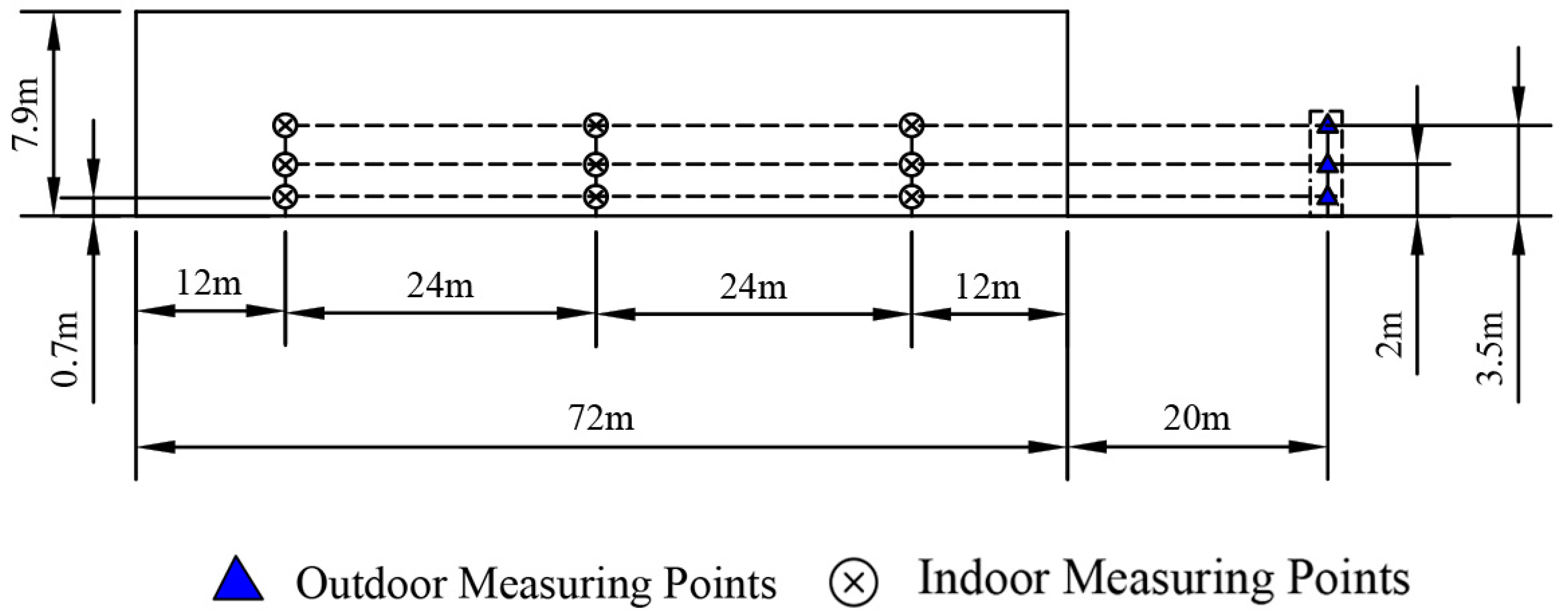
The layout of the indoor and outdoor measuring points is shown in Figure 2. In the horizontal direction, there were nine measuring points for temperature and relative humidity in the greenhouse, and one outdoor measuring point was 20 m away from the greenhouse. In the vertical direction, 3 levels were set according to the height of the cultivation plots, the middle of the plant, and the top of the plant, and the outdoor measuring points were set at the same level as shown in Figure 3. The temperature and relative humidity were automatically recorded every 10 min. The location of the light intensity measuring point was the same as that of the temperature and humidity test point, with a height of 2.0 m. Light intensity was measured every 5 min from 8:00 to 17:00 every day.
Table 1 shows the environmental monitoring sensors used in this experiment and their accuracy. The indoor and outdoor temperature, relative humidity, light intensity, and ventilation rate were recorded as the thermal and light conditions.
2.2. Modeling and Numerical Simulation
2.2.1. Environment Parameters
The light intensity in the greenhouse was the average of the measurements from 8:00 to 17:00 during the daytime. The indoor temperature and relative humidity were the averages of 27 groups of temperature and relative humidity. The outside temperature and relative humidity were the averages of 3 groups measured outside the greenhouse. In addition, the temperature and relative humidity of a certain layer in the greenhouse were the average values of 9 groups at the layer. The light rate in the greenhouse was calculated by Equation (1).
where C denotes the light rate in the greenhouse, denotes the average light intensity inside the greenhouse, and denotes the average light intensity outside the greenhouse.
The uniformity of light intensity in the greenhouse was calculated by Equation (2).
where SD represents the standard deviation of light intensity in the greenhouse and MN represents the average value of light intensity in the greenhouse.
2.2.2. Computational Domain and Meshes
The computational domain replicating the experimental setup was simulated using ANSYS-Fluent (release 2016, ANSYS, Canonsburg, PA, USA). This study used the three-dimensional (3D) steady-state method to solve the governing equations.
As shown in Figure 4, this study established a 3D geometric model of the experimental greenhouse, which took the southwest corner of the greenhouse as the coordinate origin (0,0,0), the east–west direction as the transverse direction (span direction), the north–south direction as the longitudinal direction (depth direction), the depth direction of the greenhouse as the y-axis positive direction, the span direction of the greenhouse as the x-axis positive direction, the height direction of the greenhouse as the z-axis positive direction, and the top window opening angle as a maximum of 45°.
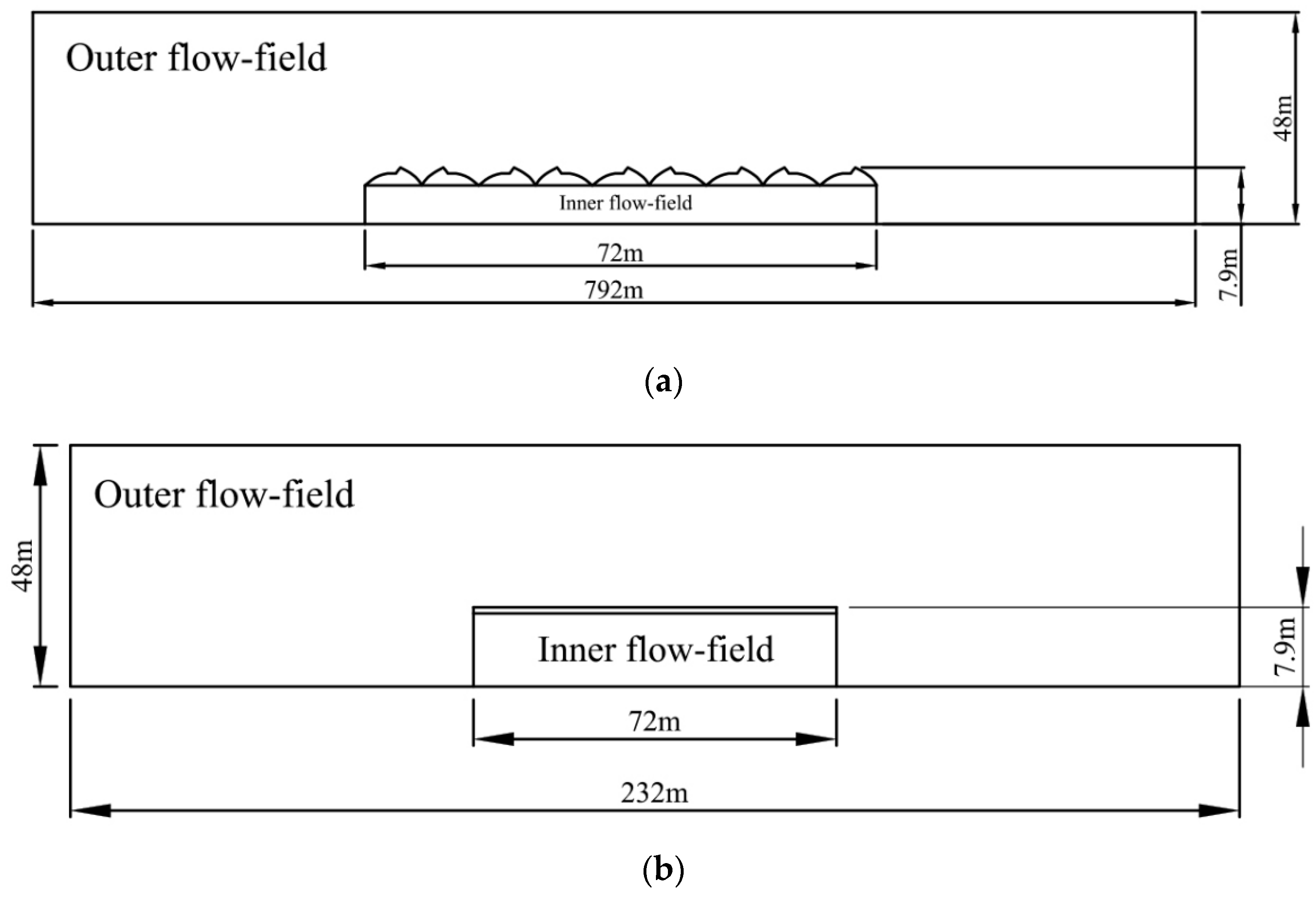
As shown in Figure 5, the greenhouse was located at the center of the external flow field, and the ground center points of the two fields coincided. The length of the external watershed was 10 times larger than the greenhouse building to ensure full development of the fluid flow process [13]. The size of the inner flow field was 72 m (L) × 72 m (W) × 7.9 m (H), and the size of the outer flow field was 792 m (L) × 232 m (W) × 48 m (H) under natural ventilation.
Considering the irregularity of the top structure of the greenhouse, this study used ICEM to divide the computational domain into unstructured grids, increase the density of the grid on the vent and wall of the greenhouse, and carry out photocoagulation treatment.
After pre-experiments, the number of grids generated was 7,130,172, the number of grid nodes was 1,162,296, the grid had no negative volume, and the grid quality was greater than 0.3. As shown in Figure 6, the grid division of the greenhouse model under natural ventilation was determined.
2.2.3. Governing Equations
The airflow in the greenhouse is a low-speed flow field at room temperature, which can be regarded as an incompressible fluid [14], and its transport process satisfies the governing equation in Equation (3):
In Equation (3), is the fluid density, is the velocity vector of , is the generalized diffusion coefficient, and is the source item.
The continuity equation is given by Equation (4) when , where is the source item of mass.
The momentum equation is given by Equations (5)–(7) when , where , and are the source items of momentum.
The energy equation is given by Equation (8) when , where T is the temperature of the airflow in the greenhouse and p is the air pressure in the greenhouse.
In Equation (8), is effective thermal conductivity given by Equation (9), where is the turbulent heat transfer coefficient determined by the turbulence model.
In Equations (10) and (11), E is the total energy of the fluid, and h is the total enthalpy of an ideal gas.
In Equation (12), is the enthalpy of the humid air transport process. And is given by Equation (13), where .
2.2.4. Numerical Model
In this study, the heat transfers and airflow in the greenhouse under natural ventilation were considered. The measured wind speed was less than 2.0 m/s, which accorded with the low-speed flow field. The airflow process in the test area was fully developed, the air in the simulated area can be regarded as a steady incompressible fluid, and the airflow conforms to Boussinesq hypothesis. In addition, the flow state of the fluid in the greenhouse was judged by the ratio of the Rayleigh number to the Prandtl number, which conformed to the turbulent motion form [6,9,14]. The standard k-ε model was selected to simulate the greenhouse under natural ventilation in Equations (14)–(16).
In Equation (14), is the eddy viscosity coefficient, k is the turbulence fluctuation kinetic energy, is the turbulence dissipation rate, and is the turbulence constant, while in Equations (15) and (16), is the laminar eddy viscosity coefficient, and are empirical constants.
In addition, solar radiation is another important factor affecting the environmental distribution in the greenhouse, and the influence of solar radiation on the microclimate in the greenhouse is closely related to the solar azimuth angle and the geographical position of the greenhouse. In this paper, discrete ordinates (DO) was the radiation model, and the radiation transfer equation is shown in Equation (17).
In Equation (17), is the solid space angle of direct sunlight, which conforms to Equation (18).
where is the solar zenith angle, is the solar azimuth, is the latitude of the test area, is the solar declination, and is the hour angle. In addition, is calculated by Equation (19).
In Equation (19), N indicates the number of days before January 1st of the current year.
In Equation (17), is the position vector, is the direction vector, is the scattering direction, s is the length along the route, is the absorption coefficient, n is the refractive index, is the scattering coefficient, is the Stefan–Boltzmann constant, I is the radiation intensity which depends on position and direction , T is the local temperature, and are phase functions.
Solar Ray Tracing (SRT) was used to load the solar-load model to calculate the solar radiation intensity, and the Solar Calculator (SC) was used to set the geographical position (109°50′ E, 18°26′ N) and time zone (GMT + 8) of Lingshui area. The trend of the greenhouse was north–south, the due north direction was y-axis positive (0,1,0), and the due east direction was x-axis positive (1,0,0).
2.2.5. Boundary Conditions
Based on the actual physical structure, the distribution of temperature and airflow in the plastic greenhouse with a semi-open roof under natural ventilation was mainly considered. The cover material in the simulation model was 0.15 mm aging-resistant polyethylene film, and the surrounding protective materials were insect-proof nets and general polyethylene film. The physical properties of the greenhouse model are shown in Table 2.
For the convenience of numerical simulation and considering the computer performance, reasonable assumptions were made after integrating the actual situation of the greenhouse. The temperature of the coating was uniformly distributed, and the heat transfer coefficient was constant. Crops cultivated in the greenhouse model were all in the seedling stage, and the transpiration was minor, ignoring the transpiration of crops in the greenhouse. The evaporation of soil in the greenhouse was ignored. The heat exchange through doors and windows in the greenhouse was not considered. Because of the large size of the experimental greenhouse, the experimental area was a part of the whole greenhouse, so all four sides of the experimental greenhouse were regarded as contacting the outside world.
As shown in Table 3, the boundary condition parameters of the experimental greenhouse numerical simulation model were set.
In addition, the protective materials around the greenhouse were an insect-proof net and general polyethylene film. The physical characteristics of the insect-proof net are shown in Table 4.
In the numerical simulation model, the insect-proof net was regarded as a one-dimensional porous medium, which was according to the Porous Jump boundary condition. According to Equation (20), the permeability coefficient K of the insect-proof net was calculated, and the porosity was obtained from Equation (21), where L denotes the mesh size of the insect-proof net and d denotes the diameter of the insect-proof net line.
2.2.6. Solution of Discrete Differential Equation
In this paper, the differential equation was solved based on the finite volume method, and its discretization format is shown in Table 5.
In the CFD module, the finite volume method was used to solve the computational domain. And the pressure-based solver was used to solve incompressible fluid flow problems in numerical simulation models. For solving discrete equations, a separate method requires less computation time, while a coupled method consumes a lot of memory, and SIMPLE algorithm is efficient in solving incompressible flow fields, so the SIMPLE algorithm was selected.
In this study, the default convergence standard of the continuity equation and momentum equation in ANSYS was lower than 10−3, and that of the energy equation was lower than 10−5. After pre-experiments, the convergence standards were determined as follows: continuity and momentum equations were 10−5, and the energy equation was 10−7. The empirical constants in Equations (14) and (16) were set as follows:
3. Results
3.1. Environment Parameter Analysis
3.1.1. Time-Variation Difference of Light Intensity
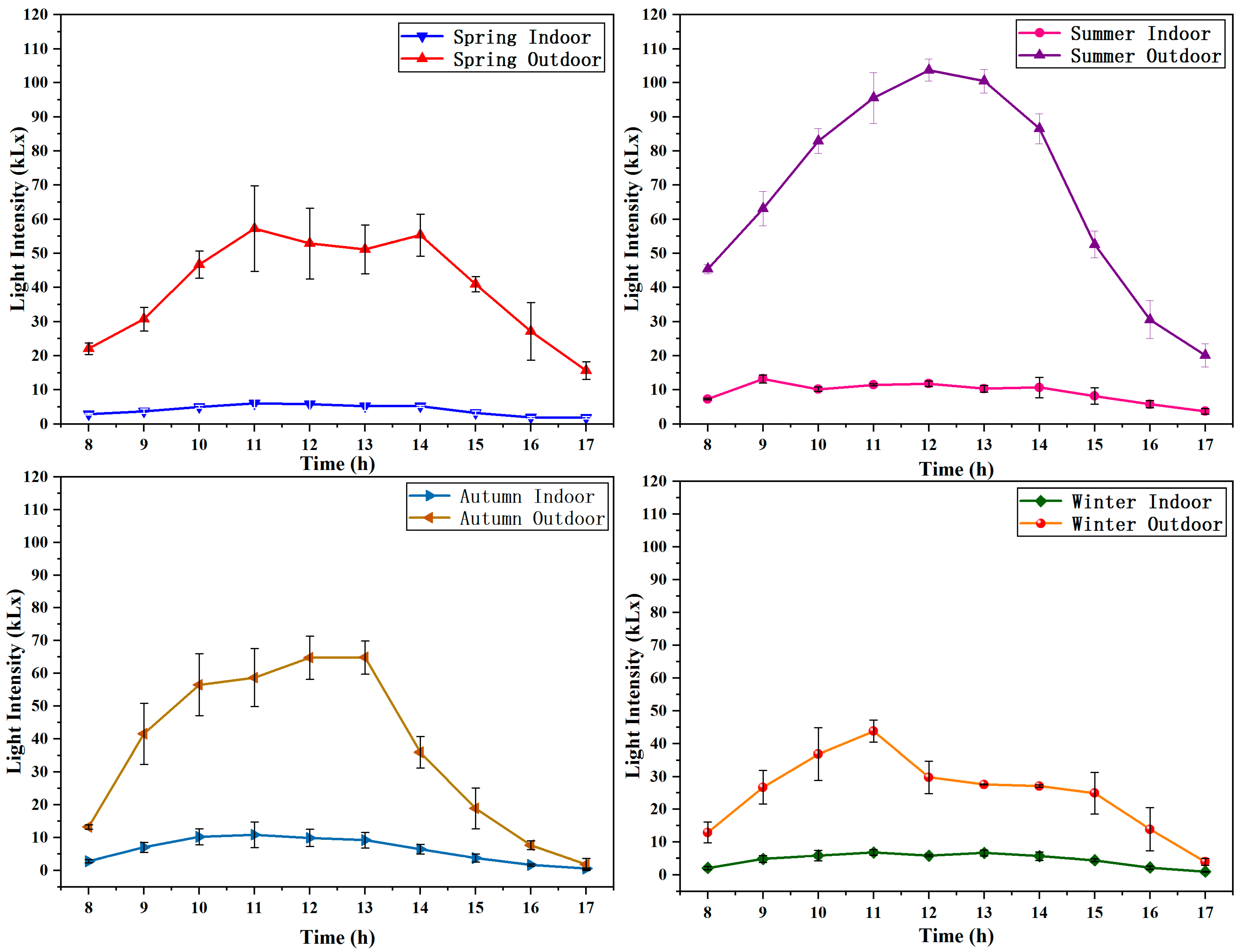
Figure 7 shows the indoor and outdoor light intensity of four seasons. Due to the influence of the external shading net, the indoor light intensity was much lower than the outdoor light intensity. Apparently, the tropical indoor light intensity in the summer and autumn was higher than that in the winter and spring, with the maximum average value of (9.3 ± 1.1) × 103 Lux in the summer and the minimum average value of (4.1 ± 0.8) × 103 Lux in the spring. The minimum light rate calculated by Equation (1) appeared lowest in the spring at 12.4%, while the maximum light rate was 16.10% in the winter. The mean coefficient of variation in the four seasons in the greenhouse was lower than 10.0%.
The daily maximum light intensity period appeared from 9:00 to 14:00, while the minimum light intensity period appeared at 8:00 and 17:00. In addition, after 15:00 in the summer and autumn, the indoor light intensity was lower than the light saturation point (LSP) of the crop. Therefore, in the actual production process, the operation time of the external shading net should be adjusted, and the sunshade net could be closed after 15:00.
3.1.2. Temperature Variation of Greenhouse
As shown in Figure 8, the greenhouse indoor temperature varied with seasons. During the experiment, the minimum ambient temperature in the Lingshui area was 18.3 °C in the winter, while the annual average temperature was 25.1 ± 0.5 °C. The maximum ambient temperature was 41.0 °C in the summer, and the annual average temperature was 31.9 ± 0.4 °C. Therefore, open-field cultivation in the Lingshui area cannot meet the temperature demand of horticultural crops, so it is necessary to carry out protected cultivation.
The average indoor temperature in the summer was 31.4 ± 0.2 °C, which was slightly lower than the indoor air temperature. During the high-temperature period from 10:00 to 14:00 in the summer, the maximum temperature difference between inside and outside the greenhouse was 2.7 °C. The maximum indoor temperature in the summer was 39.3 °C, which lagged one hour behind the outdoor peak temperature. It is common to have convective rain during the hottest summer time at noon in tropical areas, which reduces the external temperature in a short time. In the autumn, the temperature in the greenhouse was between 24 °C and 25 °C, and the maximum temperature difference between indoors and outdoors was 7.8 °C from 10:00 to 14:00. The outdoor temperature was obviously higher than the indoor temperature, mainly because the cloudy weather and the shading net blocked the sunlight and heat. The indoor temperature in the winter and spring was between 24 °C and 26 °C, and the lowest indoor temperature in the winter was 19.6 °C, which was 1.3 °C higher than the outdoor temperature. The indoor temperature difference from 19:00 to 7:00 the next day was 8.6 °C and 4.5 °C in the summer and autumn, respectively, and 6.0 °C and 4.4 °C in the winter and spring.
Figure 9 shows the temperature difference at three heights in the greenhouse. In the summer, the temperature difference between the three heights was obvious. From 9:00 to 14:00 in the summer, the minimum average temperature appeared at 3.5 m, while the maximum average temperature appeared at 2.0 m. The maximum temperature difference between these heights was 5.4 °C, which was mainly related to the solar radiation at noon, the roof vent, and the transpiration rate of the cultivated plants. In addition, the average temperature in the winter and spring increased with height and fluctuated less than 3 °C. This was mainly due to gentle temperature difference between indoors and outdoors in the winter and spring. It can be seen that with the increase in temperature in the greenhouse, the temperature difference between different layers was more significant.
3.1.3. Humidity Variation of Greenhouse
As shown in Table 6, the range of average relative humidity in the greenhouse was from 76% to 87%, and the outdoor average relative humidity was from 66% to 78%. Influenced by the covering of the greenhouse and the transpiration of plants, the indoor relative humidity was basically higher than the outdoor all year round. Therefore, the highest relative humidity in the greenhouse generally appeared at night or dawn. Along with the rise of indoor temperature during the daytime, the relative humidity in the greenhouse dropped to the lowest from 11:00 to 14:00. The difference in relative humidity indoors and outdoors varied with seasons, and the maximum difference was during summer and autumn. The maximum relative humidity difference between indoors and outdoors was 18.6% in the autumn, when there is the “dry season” of tropical monsoon climate with less rainfall and dry air. From 10:00 to 16:00 in the summer, the outdoor average temperature was 38.7 ± 0.2 °C, and the average relative humidity was 48.4 ± 0.8%, while the average temperature inside the greenhouse was 37.8 ± 0.1 °C and the average humidity was 54.5 ± 0.7%. The relative humidity was suitable for the plants, but the temperature was relatively high, causing a humid and hot indoor environment.
As shown in Figure 10, the relative humidity in the greenhouse was affected by season and height. Due to the influence of solar radiation and roof vents, the average indoor relative humidity decreased with the increase in height in the spring, autumn, and winter, and the indoor relative humidity changed in a gradient. There were great differences in relative humidity among different heights from 9:00 to 14:00 in the summer and winter. In the summer, the maximum relative humidity difference between 3.5 m and 2.0 m was 31.4%, and the maximum relative humidity difference between 3.5 m and 0.7 m was 23.7%. In the winter, the difference in relative humidity between 3.5 m and 0.7 m is obvious, and the maximum difference in relative humidity was 15.5%. At night, the average relative humidity among different heights was similar.
From the above results, it can be stated that solar radiation and natural ventilation cause the rise in the indoor temperature and the decrease in the relative humidity during the daytime, and it can be concluded that there is a coupling relationship between the three environmental factors of light intensity, air temperature, and relative humidity.
3.2. Validation Studies on CFD Simulation in Greenhouse
3.2.1. Validation of CFD Simulation Model
The simulated temperature values at the same position as the experimental measurement points were extracted from the simulation results and compared with the actual measured temperature values. By comparison, it was found that the spatial distribution law of simulated and measured values was consistent, but the simulated values of each measuring point were lower than the measured values. The maximum error between simulated and measured values appears at the test point C3 at 3.5 m height, with an error of 1.7 °C and a relative error of 5.9%. However, the measured temperature values of the whole measurement point were in agreement with the simulated values.
As shown in Table 7, the differences between the measured and simulated temperature at three heights in the greenhouse were compared, and the average relative error was 3.0%. The error between the measured values and simulated values in the engineering test was considered acceptable. Therefore, the established greenhouse CFD model is effective, the boundary conditions are set correctly, and the model can be used to further analyze the distribution law of the greenhouse environment and optimize the parameters.
3.2.2. Simulation Analysis of Greenhouse
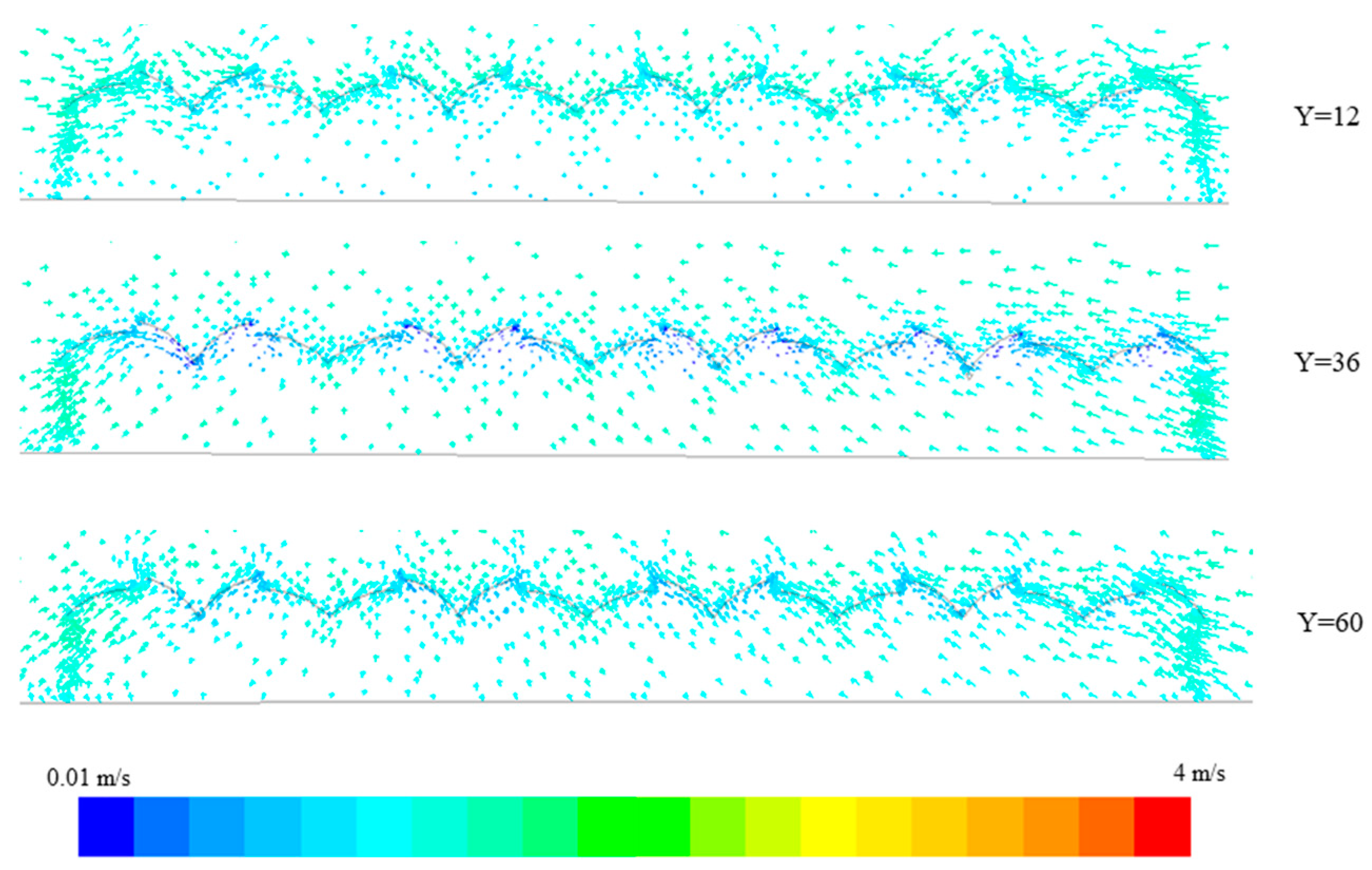
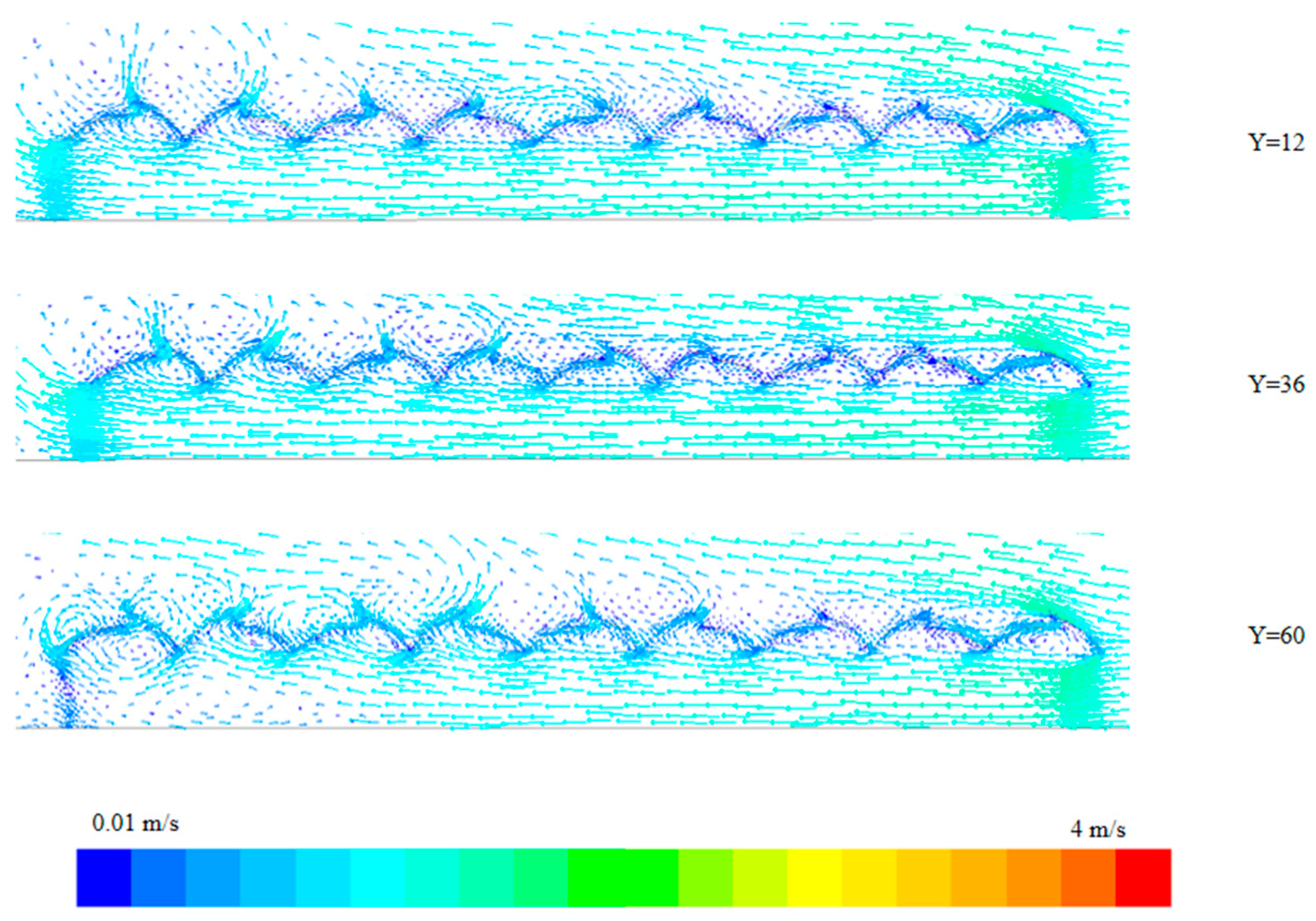
Figure 11 shows the velocity vector diagram of three sections along the depth direction of the greenhouse: 12, 36, and 60 m. It can be seen that with the increase in the horizontal distance of the greenhouse in the vertical direction, the airflow rate in the greenhouse gradually weakened. The airflow rate in the cultivation area was slow, which was not conducive to the indoor and outdoor air exchange. This distribution easily caused a high-temperature zone in the greenhouse, which affected the growth and development of cultivation. At the same time, the airflow at the inlet was blocked by the film in the upper area, which produced a vortex and increased the wind speed at the inlet.
Due to the tunnel ventilation, the vertical velocity component of the air outside the greenhouse after entering the greenhouse was minor, as shown in Figure 12. In addition, the enclosure material was an insect-proof net, so the indoor and outdoor temperature difference was small, the hot-pressing effect was not obvious, and the effect of the natural ventilation was weak.
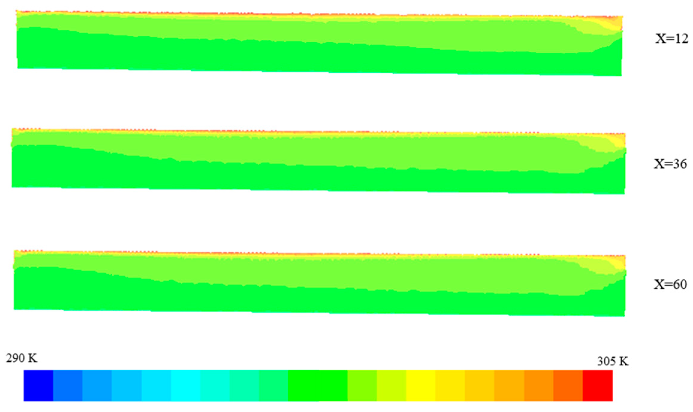
Figure 13 shows the temperature contour of three sections along the depth direction of the greenhouse: 12, 36, and 60 m. The temperature changes in the three sections were similar, the ventilation of the greenhouse is mainly limited by the external wind speed, and the indoor temperature varied with the length. Because of the effect of solar radiation, the indoor temperature increased with height. In addition, the temperature difference between different heights of the greenhouse was within 0.5 °C, and the indoor temperature field was relatively stable.
3.3. Optimization Simulation of Greenhouse
According to the simulation analysis, the combined ventilation effect of tunnel ventilation and roof ventilation was obvious. Simulation results showed that the ventilation in the greenhouse was mainly caused by wind pressure, and the temperature was greatly affected by external wind speed. To solve this problem, the temperature and flow field in the greenhouse were analyzed by changing parameters such as the configuration and opening size of the windows and the external wind speed, which would affect the natural ventilation of the greenhouse. Therefore, the established CFD model of the greenhouse was used to analyze the influence of the above parameters on the natural ventilation of the greenhouse, hopefully to provide a theoretical basis for the environmental control and optimization of large-scale film greenhouses in tropical areas.
3.3.1. Greenhouse Ventilation Simulation
The roof film of the windward surface of the greenhouse was modified to an insect-proof net to increase the ventilation area, and the other surfaces remained the same, with the previous settings. In the improved model, the changes in temperature and flow field in the greenhouse were analyzed.
As shown in Figure 14, with the increased vents, turbulence disappeared in the greenhouse. In the longitudinal direction of the greenhouse, the maximum difference in flow velocity between 0.7 m, 2.0 m, and 7.5 m was about 0.05 m/s, and the airflow distribution in the greenhouse was relatively stable, with an average velocity of 1.3 m/s. In the Y direction of the greenhouse, the top airflow velocity in the second half decreased and was mainly affected by the length of the greenhouse.
Figure 15 shows the temperature in the greenhouse was evenly distributed in the lateral direction. The top of the greenhouse was affected by external solar radiation in the vertical direction; therefore, the temperature in the greenhouse increases with height.
3.3.2. Greenhouse Ventilation Optimizations
Figure 16 shows the flow field distribution of the combined ventilation of side and roof windows. By increasing the open area of the side windows, the overall airflow of the greenhouse was improved. The flow field distributions of Y = 12 m, Y = 36 m, and Y = 60 m sections in the greenhouse were basically the same, and the average velocity of airflow in the greenhouse was 0.6 m/s. In addition, the increase in the open area of the side windows both strengthened the cross ventilation and affected the thermal pressure ventilation. Therefore, the air velocity near the top window reached from 0.5 m/s to 1 m/s.
As shown in Figure 17, in the direction parallel to the greenhouse, the temperature distribution of the three sections had certain differences. Under the influence of solar radiation, the temperature change increases with the increase in height in the longitudinal direction, and the temperature difference at X = 12 section in the transverse direction was large.
3.3.3. External Airflow Simulation
By comparing the experiment and simulation results, it can be concluded that the ventilation efficiency of the greenhouse was mainly affected by the wind pressure ventilation, so increasing the outdoor ventilation rate could improve the airflow of the greenhouse. Figure 18 shows the indoor airflow vector diagram for the outdoor wind speed of 3 m/s.
With the increase in greenhouse length, the speed gradually decreased, so the ventilation in the greenhouse was mainly affected by the external wind speed. When the wind speed was 3 m/s, the indoor air velocity increased, and there was an obvious gradient change in the vertical direction, where the average velocity of the airflow at the height of 2.0 m in the greenhouse was the maximum, reaching 2.1 m/s. The airflow from the gutter to the roof was evenly distributed under the influence of greenhouse covers. Therefore, in a tropical area, it is recommended to design the greenhouse according to the summer wind direction to make full use of the natural ventilation.
As shown in Figure 19, when the external wind speed was 3 m/s, the indoor temperature distribution trend was consistent in the lateral direction, and the temperature gradually increased in the vertical direction, which was mainly affected by solar radiation and airflow speed in the greenhouse. At the same time, the plastic film on the greenhouse roof played an obstructing role, which made the temperature in the top area at the entrance of the vent slightly higher.
3.3.4. Optimization Schemes
By comparing the optimization modes of enlarging the size of roof vents, increasing side windows, and changing the external wind speed, the indoor air velocity gradually increased with the external wind speed, which had an obvious turbulent effect on the indoor air velocity at different heights. When the size of greenhouse vents was increased, the air velocity at the height of 2.0 m was the maximum, the relative velocity at both sides was small, and the overall air velocity in the greenhouse was relatively uniform. In addition, changing the configuration of vents also had a certain effect on the distribution of air velocity in the greenhouse. By increasing the open area of side windows, the utilization rate of roof vents would be improved, and the ventilation rate in the greenhouse could be increased.
Therefore, the spatial distribution of microclimate in the greenhouse is affected by the external wind speed, the configuration of vents, and the size of vents. The optimization scheme of designing the orientation of the greenhouse according to the maximum air volume in the summer can improve the utilization efficiency of natural ventilation, and increasing the size of greenhouse vents and adding side windows can be selectively used in the winter and spring.
4. Discussion
A plastic greenhouse with a semi-open roof is mainly used to produce truss tomatoes and mini watermelons in tropical areas. Therefore, this study mainly analyzes the annual production environment of this greenhouse. Compared with the gothic arch greenhouse [15] and Venlo-type greenhouse [16], a plastic greenhouse with a semi-open roof exhibits a high natural ventilation efficiency and lower cooling energy consumption in the summer. A semi-open ventilation structure, which increases the air exchange rate of the greenhouse, is adopted for the roof, and the north–south trend improves the overall light uniformity, which is beneficial to annual production.
The light intensity in the plastic greenhouse was significantly lower than the outdoor natural light due to the influence of roof angle, frame structure, plastic film characteristics, and other factors. Due to the influence of the shading net, the indoor light conditions of four seasons cannot meet the growth needs, which is different from the research results of Singh et al. [17] and is mainly related to the cleanliness of the greenhouse structure and covering materials. At the same time, the solar radiation received by the greenhouse in the south–north direction was lower than that in the east–west direction, but the sunlight received by the greenhouse was more uniform throughout the year [18].
The indoor temperature is strongly affected by solar radiation and the ambient air temperature, and the highest indoor temperature during the experiment reached 39.3 °C in the summer, lagging behind the outdoor temperature by one hour, which is similar to the results of Badji et al. [19]. The indoor temperature is still higher than the suitable temperature for the crops in the greenhouse, so additional ventilation and cooling measures are needed. The relative humidity in the test greenhouse was lower than that of the solar greenhouse and plastic greenhouse because of the large area of the side windows and the top windows with a long time of opening. However, the relative humidity in the test greenhouse changed slowly, which was due to the larger volume of the test greenhouse and higher humidity inertia.
In this study, different numbers and types of grids were selected for comparative analysis in the process of meshing. Pre-experiments showed that it was faster to transform unstructured grids into polyhedral grids for calculation within the applicable scope of computers, which was in agreement with the research results of Banakar et al. [20]. In addition, for the selection of boundary conditions in the process of simulating natural ventilation in the greenhouse, two sides were set as symmetry boundary conditions in this paper, which is different from the periodic boundary conditions set by Deng et al. [21], mainly because of the differences between the actual conditions of the two physical models, which cannot be considered equally. Furthermore, the thermal environment simulation error of the numerical simulation model constructed in this study was 3.0%, which is far less than the allowable range of 20% in engineering simulations. This result is similar to those of Liang et al. [22], in which the maximum relative error of temperature simulation was 3.71%. Compared with the dynamic simulation model, the three-dimensional steady-state model used in this study provides a lower computational load, and its accuracy is close to that of Liang and Xu et al. [23].
According to the optimization simulation results of the greenhouse CFD model, optimizing the size and configuration of vents can promote roof ventilation efficiency, which is in agreement with the results of Villagran et al. [6] on natural ventilation of traditional Colombian greenhouses, gothic multi-span greenhouses, and curved multi-span greenhouses in tropical areas. In addition, the optimization scheme proposed in this study is superior to the results of Singhal et al. [24] and Fan et al. [25] in terms of large-scale environmental uniformity and natural ventilation efficiency. At the same time, when the wind speed outside the greenhouse is low, the influence of wind direction on natural ventilation is as important as that of wind speed, which is consistent with the research results of Bournet et al. Moreover, compared with the results of Lu et al. [26], who used multifunctional fan-coil unit systems in Chinese solar greenhouses, this study had higher energy efficiency by increasing the vent size and adopting the top window, which improved the uniformity of the thermal environment in the greenhouse and the efficiency of natural ventilation without additional mechanical equipment.
5. Conclusions
This study evaluated the environmental parameters of a plastic greenhouse with a semi-open roof in a tropical area in four seasons and optimized the vent structure of the greenhouse based on CFD simulation. The following conclusions were drawn:
- In this study, the temperature, relative humidity, and light intensity in different seasons were analyzed for a plastic greenhouse with a semi-open roof. The maximum indoor temperature in the summer was 39.3 °C, and the average indoor temperature in the summer was 31.4 ± 0.2 °C, while the average indoor temperature was between 24 °C and 26 °C in the other three seasons; the minimum indoor temperature in the winter was 19.6 °C. The average relative humidity was 76–87% annually. The average indoor light intensity varied less than 10.0% in four seasons.
- The three-dimensional steady-state CFD model of a multi-span plastic greenhouse under natural ventilation was established. The maximum relative error (MRE) of the model between the simulated and measured values of the temperature at the measuring point in the greenhouse was 5.9%, and the average relative error was 3.0%.
- Increasing side windows and roof vents can make full use of natural wind and achieve a better energy-saving effect by reducing the usage of mechanical ventilation systems. With the increase in vent size, the indoor airflow distribution was stable, and the average velocity airflow was 1.3 m/s.
- The indoor airflow was homogenized and improved by increasing the side window area, after which the average velocity of indoor air was 1.4 m/s, and the ventilation efficiency of the roof window was improved. When the inlet wind speed of the greenhouse was increased to 3.0 m/s, the average velocity at the cultivation area reached 2.1 m/s. Furthermore, it is recommended that future studies include different types of plants within the CFD model since the developed plants will generate thermal changes of different airflow patterns from those found in this study.
Author Contributions
H.Y.: conceptualization, methodology, formal analysis, writing—original draft, writing—review and editing, visualization. K.W.: software, writing—review and editing. H.Y. and K.W. contributed equally to this work. J.Z.: software, data curation, resources. Z.P.: methodology, project administration, writing—review and editing, Funding acquisition. All authors have read and agreed to the published version of the manuscript.
Funding
This research was funded by the Hainan Province Science and Technology Special Fund (ZDYF2023XDNY044).
Informed Consent Statement
This study was performed by the authors, and no participants other than the authors were involved in it; informed consent was obtained from all authors.
Data Availability Statement
Data will be made available on request.
Acknowledgments
The author would like to thank all the anonymous reviewers for their helpful comments and suggestions and Geqi Yan B.E. for help and contribution to the field experiment.
Conflicts of Interest
The authors declare no conflicts of interest.
Nomenclature
| C | Daylighting rate in greenhouse | Source item | |
| CFD | Computational fluid dynamics | Universal variable | |
| CV | Coefficient of variation | Source item of mass | |
| Average illumination intensity inside the greenhouse | T | Temperature of airflow | |
| Average illumination intensity outside the greenhouse | p | Air pressure | |
| SD | Standard deviation | Effective thermal conductivity | |
| MN | Average value of light intensity | Turbulent heat transfer coefficient | |
| SRT | Solar Ray Tracing | E | Total energy of fluid |
| Fluid density | h | Total enthalpy of ideal gas | |
| Velocity vector of | Enthalpy of humid air transport process | ||
| Generalized diffusion coefficient | Reference temperature | ||
| Eddy viscosity coefficient | k | Turbulence fluctuation kinetic energy | |
| Turbulence dissipation rate | Turbulence constant | ||
| Laminar eddy viscosity coefficient | Empirical constants | ||
| Solid space angle of direct sunlight | Solar zenith angle | ||
| Solar azimuth | Latitude of the test area | ||
| Solar declination | Hour angle | ||
| The number of days before January 1st of thecurrent year | Position vector | ||
| Direction vector | Scattering direction | ||
| s | Length along the route | Absorption coefficient | |
| n | Refractive index | Scattering coefficient | |
| Stefan–Boltzmann constant | I | Radiation intensity | |
| K | Permeability coefficient | Phase functions | |
| L | Mesh size of insect-proof net | Porosity of insect-proof net | |
| d | Diameter of the insect-proof net line |
References
- Chen, W.H.; Mattson, N.S.; You, F. Intelligent control and energy optimization in controlled environment agriculture via nonlinear model predictive control of semi-closed greenhouse. Appl. Energy 2022, 320, 119334. [Google Scholar] [CrossRef]
- Ma, D.; Carpenter, N.; Maki, H.; Rehman, T.U.; Tuinstra, M.R.; Jin, J. Greenhouse environment modeling and simulation for microclimate control. Comput. Electron. Agric. 2019, 162, 134–142. [Google Scholar] [CrossRef]
- Li, A.; Huang, L.; Zhang, T. Field test and analysis of microclimate in naturally ventilated single-sloped greenhouses. Energy Build. 2017, 138, 479–489. [Google Scholar] [CrossRef]
- Bay, E.; Martinez-Molina, A.; Dupont, W.A. Assessment of natural ventilation strategies in historical buildings in a hot and humid climate using energy and CFD simulations. J. Build. Eng. 2022, 51, 104287. [Google Scholar] [CrossRef]
- Lee, S.Y.; Lee, I.B.; Kim, R.W. Evaluation of wind-driven natural ventilation of single-span greenhouses built on reclaimed coastal land. Biosyst. Eng. 2018, 171, 120–142. [Google Scholar] [CrossRef]
- Villagran, E.A.; Romero, E.J.B.; Bojacá, C.R. Transient CFD analysis of the natural ventilation of three types of greenhouses used for agricultural production in a tropical mountain climate. Biosyst. Eng. 2019, 188, 288–304. [Google Scholar] [CrossRef]
- Soussi, M.; Chaibi, M.T.; Buchholz, M.; Saghrouni, Z. Comprehensive review on climate control and cooling systems in greenhouses under hot and arid conditions. Agronomy 2022, 12, 626. [Google Scholar] [CrossRef]
- Tawalbeh, M.; Aljaghoub, H.; Alami, A.H.; Olabi, A.G. Selection criteria of cooling technologies for sustainable greenhouses: A comprehensive review. Therm. Sci. Eng. Prog. 2013, 38, 101666. [Google Scholar] [CrossRef]
- Wu, X.; Li, Y.; Jiang, L.; Wang, Y.; Liu, X.; Li, T. A systematic analysis of multiple structural parameters of Chinese solar greenhouse based on the thermal performance. Energy 2023, 273, 127193. [Google Scholar] [CrossRef]
- Liu, J.; Wu, X.; Sun, F.; Wang, B. Development and Application of a Crossed Multi-Arch Greenhouse in Tropical China. Agriculture 2022, 12, 2164. [Google Scholar] [CrossRef]
- McCartney, L.; Orsat, V.; Lefsrud, M.G. An experimental study of the cooling performance and airflow patterns in a model Natural Ventilation Augmented Cooling (NVAC) greenhouse. Biosyst. Eng. 2018, 174, 173–189. [Google Scholar] [CrossRef]
- Flores-Velázquez, J.; Rojano, F.; Aguilar-Rodríguez, C.E.; Villagran, E.; Villarreal-Guerrero, F. Greenhouse Thermal Effectiveness to Produce Tomatoes Assessed by a Temperature-Based Index. Agronomy 2022, 12, 1158. [Google Scholar] [CrossRef]
- Wang, X.W.; Luo, J.Y.; Li, X.P. CFD based study of heterogeneous microclimate in a typical Chinese greenhouse in central China. J. Integr. Agric. 2013, 12, 914–923. [Google Scholar] [CrossRef]
- Paing, S.T.; Anderson, T.N. Characterizing the effects of geometry on the natural convection heat transfer in closed even-span gable-roof greenhouses. Therm. Sci. Eng. Prog. 2024, 48, 102408. [Google Scholar] [CrossRef]
- Hashemi, S.F.; Pourfallah, M.; Gholinia, M. Thermal performance enhancement in an indirect solar greenhouse dryer using helical fin under variable solar irradiation. Sol. Energy 2024, 267, 112217. [Google Scholar] [CrossRef]
- Yan, H.; Deng, S.; Zhang, C.; Wang, G.; Zhao, S.; Li, M.; Zhou, Y. Determination of energy partition of a cucumber grown Venlo-type greenhouse in southeast China. Agric. Water Manag. 2023, 276, 108047. [Google Scholar] [CrossRef]
- Singh, M.C.; Kaur, P.; Singh, J.P.; Singh, K.G.; Singh, A. Postharvest Physicochemical Quality Assessment of Greenhouse Produced Soilless Cucumbers in Relation to Differential Fertigation. J. Agric. Eng. 2023, 60, 38–50. [Google Scholar]
- Bo, Y.; Zhang, Y.; Zheng, K.; Zhang, J.; Wang, X.; Sun, J.; Wang, J. Light environment simulation for a three-span plastic greenhouse based on greenhouse light environment simulation software. Energy 2023, 271, 126966. [Google Scholar] [CrossRef]
- Badji, A.; Benseddik, A.; Bensaha, H.; Boukhelifa, A.; Hasrane, I. Design, technology, and management of greenhouse: A review. J. Clean. Prod. 2022, 373, 133753. [Google Scholar] [CrossRef]
- Banakar, A.; Montazeri, M.; Ghobadian, B.; Pasdarshahri, H.; Kamrani, F. Energy analysis and assessing heating and cooling demands of closed greenhouse in Iran. Therm. Sci. Eng. Prog. 2021, 25, 101042. [Google Scholar] [CrossRef]
- Deng, L.; Huang, L.; Zhang, Y.; Li, A.; Gao, R.; Zhang, L.; Lei, W. Analytic model for calculation of soil temperature and heat balance of bare soil surface in solar greenhouse. Sol. Energy 2023, 249, 312–326. [Google Scholar] [CrossRef]
- Liang, Z.; Xu, L.; De Baerdemaeker, J.; Li, Y.; Saeys, W. Optimization of a multi-duct cleaning device for rice combine harvesters utilizing CFD and experiments. Biosyst. Eng. 2020, 190, 25–40. [Google Scholar] [CrossRef]
- Xu, T.; Zhou, H.; Lv, X.; Lei, X.; Tao, S. Study of the distribution characteristics of the airflow field in tree canopies based on the CFD model. Agronomy 2022, 12, 3072. [Google Scholar] [CrossRef]
- Singhal, S.; Yadav, A.K.; Prakash, R. Numerical modelling of an earth-air-tunnel assisted single span saw-tooth greenhouse for tropical climate. Int. J. Therm. Sci. 2023, 187, 108138. [Google Scholar] [CrossRef]
- Fan, Z.; Li, Y.; Jiang, L.; Wang, L.; Li, T.; Liu, X. Analysis of the Effect of Exhaust Configuration and Shape Parameters of Ventilation Windows on Microclimate in Round Arch Solar Greenhouse. Sustainability 2023, 15, 6432. [Google Scholar] [CrossRef]
- Lu, J.; Li, H.; He, X.; Zong, C.; Song, W.; Zhao, S. CFD Simulation and Uniformity Optimization of the Airflow Field in Chinese Solar Greenhouses Using the Multifunctional Fan–Coil Unit System. Agronomy 2023, 13, 197. [Google Scholar] [CrossRef]
Figure 1.
Experimental greenhouse.

Figure 2.
Schematic of measuring points in the horizontal direction (A, B and C was the group serial number of measuring points).
Figure 2.
Schematic of measuring points in the horizontal direction (A, B and C was the group serial number of measuring points).

Figure 3.
Schematic of measuring points in the vertical direction.

Figure 4.
Geometric model of greenhouse.

Figure 5.
The front view (a) and side view (b) of the internal and external airflow fields.

Figure 6.
Global grid division of greenhouse model.

Figure 7.
Indoor and outdoor light intensity of greenhouse in four seasons.

Figure 8.
Indoor and outdoor average air temperature of greenhouse in four seasons.

Figure 9.
Temperature variation of different heights (0.7 m, 2.0 m, 3.5 m) in four seasons.

Figure 10.
Relative humidity variation of different heights (0.7 m, 2.0 m, 3.5 m) in different seasons.
Figure 10.
Relative humidity variation of different heights (0.7 m, 2.0 m, 3.5 m) in different seasons.

Figure 11.
Velocity on X sections (X = 12 m, X = 36 m, X = 60 m).

Figure 12.
Velocity on Y sections (Y = 12 m, Y = 36 m, Y = 60 m).

Figure 13.
Temperature contour on X sections (X = 12 m, X = 36 m, X = 60 m).

Figure 14.
Vector diagram of airflow in greenhouse with increased vents on X sections (X = 12 m, X = 36 m, X = 60 m).
Figure 14.
Vector diagram of airflow in greenhouse with increased vents on X sections (X = 12 m, X = 36 m, X = 60 m).

Figure 15.
Temperature in contour greenhouse with increased vents on X sections (X = 12 m, X = 36 m, X = 60 m).
Figure 15.
Temperature in contour greenhouse with increased vents on X sections (X = 12 m, X = 36 m, X = 60 m).

Figure 16.
Vector diagram of airflow distribution in greenhouse with side window (Y = 12, Y = 36, Y = 60).
Figure 16.
Vector diagram of airflow distribution in greenhouse with side window (Y = 12, Y = 36, Y = 60).

Figure 17.
Temperature contour in greenhouse with side window (X = 12 m, X = 36 m, X = 60 m).

Figure 18.
Vector diagram of external wind speed at 3 m/s (X = 12 m, X = 36 m, X = 60 m).

Figure 19.
Temperature contour in the greenhouse with external wind speed at 3 m/s (X = 12 m, X = 36 m, X = 60 m).
Figure 19.
Temperature contour in the greenhouse with external wind speed at 3 m/s (X = 12 m, X = 36 m, X = 60 m).


Table 1.
Information of environment monitoring sensors.
| Environment Parameter | Instrument Model | Precision |
|---|---|---|
| Air Temperature | HOBO | 0.2 °C |
| Relative Humidity | HOBO | ±2.5% Rh |
| Illumination Intensity | Top Cloud-agri TPJ-22-G | ±2% FS |
| Roof Temperature | Fluke F59 | ±2.0 °C |
| Airflow Velocity | Kestrel4000 | 0.10 m/s |
Table 2.
Material properties in greenhouse.
| Physical Parameter | Air | Plastic Film | Soil |
|---|---|---|---|
| Density (kg·m−3) | 1.22 | 923 | 1900 |
| Specific Heat Capacity (J · (kg · K)−1) | 1006.43 | 2300 | 2200 |
| Thermal Conductivity | 0.0242 | 0.38 | 2.00 |
| Absorption Coefficient | 0.19 | 0.37 | 0.50 |
| Scattering Coefficient | 0.00 | 0.30 | 1.00 |
| Refractive Index | 1.00 | 1.92 | - |
| Emissivity | 0.86 | 0.80 | 0.90 |
Table 3.
Boundary condition settings.
| Parameter | Setting | Value |
|---|---|---|
| Windward Side | Velocity Entrance | 1.4 m/s |
| Leeward Side | Pressure Outlet | 101,325 Pa |
| Top Side | Plastic | -- |
| Air | Temperature | 302.75 K |
Table 4.
Physical properties of insect-proof net.
| Parameter | Value |
|---|---|
| Diameter of the line | 0.18 mm |
| Porosity | 0.41 |
| Mesh size | 0.5 mm × 0.5 mm, 40-mesh |
| Permeability coefficient | 8.26 × 10⁻¹⁰ m2 |
| Resistance coefficient | 1.89 |
Table 5.
Selection of discrete scheme.
| Pressure Dispersion | Energy Dispersion | Momentum Dispersion | k Dispersion | ε Dispersion |
|---|---|---|---|---|
| Mass–force weighting | Second-order upwind | Second-order upwind | First-order upwind | First-order upwind |
Table 6.
Relative humidity of the greenhouse in four seasons (0:00–24:00).
| Season | Maximum (%) | Minimum (%) | Average ± SE (%) | |||
|---|---|---|---|---|---|---|
| Indoor | Outdoor | Indoor | Outdoor | Indoor | Outdoor | |
| Spring | 99.0 | 98.0 | 58.3 | 50.3 | 86.5 ± 0.2 | 77.9 ± 0.9 |
| Summer | 97.1 | 96.1 | 40.2 | 40.6 | 76.6 ± 0.6 | 71.2 ± 2.2 |
| Autumn | 92.0 | 91.3 | 42.9 | 26.0 | 79.0 ± 0.2 | 66.4 ± 1.0 |
| Winter | 98.4 | 98.4 | 46.3 | 43.7 | 82.7 ± 0.3 | 73.5 ± 1.0 |
Table 7.
Comparison between measured and simulated average temperature at three heights.
| Height (m) | Measured Average Temperature (°C) | Simulated Average Temperature (°C) | Relative Error (%) |
|---|---|---|---|
| 0.7 | 26.5 | 26.2 | 2.5 |
| 2.0 | 27.0 | 26.3 | 2.8 |
| 3.5 | 27.5 | 26.4 | 3.9 |
Disclaimer/Publisher’s Note: The statements, opinions and data contained in all publications are solely those of the individual author(s) and contributor(s) and not of MDPI and/or the editor(s). MDPI and/or the editor(s) disclaim responsibility for any injury to people or property resulting from any ideas, methods, instructions or products referred to in the content. |
© 2024 by the authors. Licensee MDPI, Basel, Switzerland. This article is an open access article distributed under the terms and conditions of the Creative Commons Attribution (CC BY) license (https://creativecommons.org/licenses/by/4.0/).
Share and Cite
MDPI and ACS Style
Yin, H.; Wang, K.; Zeng, J.; Pang, Z. CFD Analysis and Optimization of a Plastic Greenhouse with a Semi-Open Roof in a Tropical Area. Agronomy 2024, 14, 876. https://doi.org/10.3390/agronomy14040876
AMA Style
Yin H, Wang K, Zeng J, Pang Z. CFD Analysis and Optimization of a Plastic Greenhouse with a Semi-Open Roof in a Tropical Area. Agronomy. 2024; 14(4):876. https://doi.org/10.3390/agronomy14040876
Chicago/Turabian StyleYin, Haoran, Kaiji Wang, Jiadong Zeng, and Zhenzhen Pang. 2024. "CFD Analysis and Optimization of a Plastic Greenhouse with a Semi-Open Roof in a Tropical Area" Agronomy 14, no. 4: 876. https://doi.org/10.3390/agronomy14040876
Note that from the first issue of 2016, this journal uses article numbers instead of page numbers. See further details here.