Cotton Water Use Efficiency under Two Different Deficit Irrigation Scheduling Methods

Abstract

Declines in Ogallala aquifer levels used for irrigation has prompted research to identify methods for optimizing water use efficiency (WUE) of cotton (Gossypium hirsutum L). In this experiment, conducted at Lubbock, TX, USA in 2014, our objective was to test two canopy temperature based stress indices, each at two different irrigation trigger set points: the Stress Time (ST) method with irrigation triggers set at 5.5 (ST_5.5) and 8.5 h (ST_8.5) and the Crop Water Stress Index (CWSI) method with irrigation triggers set at 0.3 (CWSI_0.3) and 0.6 (CWSI_0.6). When these irrigation triggers were exceeded on a given day, the crop was deficit irrigated with 5 mm of water via subsurface drip tape. Also included in the experimental design were a well-watered (WW) control irrigated at 110% of potential evapotranspiration and a dry land (DL) treatment that relied on rainfall only. Seasonal crop water use ranged from 353 to 625 mm across these six treatments. As expected, cotton lint yield increased with increasing crop water use but lint yield WUE displayed asignificant (p ≤ 0.05) peak near 3.6 to 3.7 kg ha⁻¹ mm⁻¹ for the ST_5.5 and CWSI_0.3 treatments, respectively. Our results suggest that WUE may be optimized in cotton with less water than that needed for maximum lint yield.

1. Introduction

Limited soil water availability reduces crop growth more than all other environmental factors combined [1]. Depletion of ground water resources for irrigation, as is the case with the Ogallala aquifer on the US Southern High Plains [2], places a premium on irrigation scheduling methods that improve crop water use efficiency (WUE). Hatfield et al. [3] surveyed the literature and found large variations in measured WUE across climates, crops and soil management practices.

Drought stress reduces stomatal conductance and this in turn reduces latent energy removal from the crop causing canopy temperature (T_c) to rise relative to a well-watered, freely transpiring crop. In addition to a lack of water, several environmental [4,5,6] as well as morphological and physiological [7,8,9] factors combine to determine the canopy energy balance and the specific value of T_c at any given instant. The T_c is a relatively easy to acquire general indicator of drought stress and as a result, this measurement has been used in various irrigation scheduling strategies [10,11]. The Stress Time (ST) method of irrigation scheduling accumulates the amount of daily time that T_c exceeds a specified optimum or threshold T_c for a crop. This threshold temperature is generally assumed to be about 28 °C for cotton [12]. Under the ST index criteria, irrigation is triggered when T_c exceeds this threshold temperature for a specified duration of time, called the time threshold, during a given day [13,14].

Another irrigation scheduling method that uses measured T_c is the Crop Water Stress Index (CWSI) [15,16]. This method requires the development of a non-water stressed baseline, which is the linear relationship between the canopy minus air temperature differential (T_c − T_a) vs. air vapor pressure deficit (VPD) under non-limiting soil water conditions, where the crop is transpiring at the potential rate. A second or upper base line represents the T_c − T_a of a non-transpiring crop that is insensitive to VPD. The CWSI varies from 0 to 1 with 0 indicating maximum transpiration and no drought stress and 1 indicating no transpiration and maximum drought stress. The CWSI has subsequently been related to other physical and physiological measures of drought stress, including soil water content [16], plant water potential [17,18], and net photosynthesis [19,20]. In this paper, seed cotton water use efficiency is defined as the mass of dry seed cotton (e.g., seed + lint) per unit crop water use over the season. Similarly, lint yield water use efficiency is defined here as dry lint yield per unit crop water use over the season. Our objectives were to compare irrigation timing, cotton yield, crop water use and WUE over a range of water regimes using the ST and CWSI methods of deficit irrigation scheduling.

2. Materials and Methods

Six individually controlled irrigation zones used in this experiment were located at Lubbock, TX, USA (33°35′40.87′′ N, 101°53′51.75′′ W). Each zone consisted of 8 north-south oriented rows, spaced 1.0 m apart with subsurface drip irrigation (SDI) tape located 0.4 m below the soil surface. Cotton (Gossypium hirsutum L) cultivar cv. FM 9058F (FiberMax, Bayer CropScience, Research Triangle Park, NC, USA) was planted on June 2, 2014 (Day of Year (DOY) 153). On DOY 182, plants were thinned to a uniform plant population of 90,000 plants ha⁻¹ and three 5 m lengths of row in each of the six irrigation plots were staked and designated for instrumentation placement and final yield determination.

The soil was an Amarillo fine sandy loam (fine-loamy, mixed, superactive, thermic Aridic Paleustalfs). Urea ammonium nitrate was delivered through the SDI system by injecting a concentrated solution of ammonium sulfate (30–0–0) metered to deliver 4.5 kg ha⁻¹ cm⁻¹ available N per cm irrigation water applied. Automated irrigations began on DOY 202 and ended DOY 272. During this period, N fertilizer injection began DOY 191 and ended DOY 212.

Six water treatments were imposed in this experiment: One Well Watered (WW), one Dry Land (DL), two Stress Time (ST) treatments and two Crop Water Stress Index (CWSI) treatments, described in detail below. Canopy temperatures (T_c) were measured on a section of row designated for final lint yield determination in one of the three replicates of each water treatment. These T_c measurements were used to control irrigation for ST and CWSI treatments. In all six water treatments, two infrared thermometers IRTs (Apogee IRT model SI-121, Apogee Instruments Inc., Logan, UT, USA were mounted on an adjustable mast oriented at ~30° from horizontal to measure T_c. Mention of this or other proprietary products is for the convenience of the readers only, and does not constitute endorsement or preferential treatment of these products by USDA-ARS. USDA is an equal opportunity provider and employer.) Both IRTs were placed 15 cm from center of the row target. This provides a field of view of about 9.7 cm. A data logger (CR 23X, Campbell Scientific Inc., Logan, UT, USA) connected to a data logger multiplexer (AM16/32B, Campbell Scientific Inc., Logan, UT, USA) was used to measure and record data from the IRTs as well as measuring air temperature (T_a) and vapor pressure deficit (VPD) (Air temperature/humidity probe model HMP45C-L, Campbell Scientific Inc., Logan, UT, USA) and photosynthetically active radiation (PAR) (LI-190, LICOR, Inc., Lincoln, NE, USA). These data were measured each second and averaged and recorded every 15 min. Daily total solar irradiance (LI 200X, LICOR, Inc., Lincoln, NE, USA) and rainfall (Rain gauge model TE-525, Campbell Scientific, Logan, UT, USA) were obtained from a nearby weather station.

Prior to planting, the entire field was watered to field capacity to insure soil water uniformity at the outset of the experiment. Before planting and after harvest, soil water content was determined gravimetrically to a depth of 1m in three replicate locations within each irrigation zone. These 1 m deep by 25.4 mm diameter soil cores were extracted with a tractor mounted hydraulic soil coring and sampling machine (Giddings Machine Company, Windsor, CO, USA). These pre- and post-season measurements of soil water content were used along with rainfall totals and irrigation amounts to estimate crop water use over the growing season. Irrigation application treatments began and ended on DOY 202 and 272, respectively. The WW plots were watered several times per week with an amount of water equal to 110% of potential evapotranspiration (PET) over that time period. Daily PET was taken from the Texas Tech Mesonet web page (http://www.mesonet.ttu.edu/Tech/1-output/climate.html). This station (33.604091 N, 101.899195 W) is located about 1 km N of the Lubbock field site. The DL treatment received no supplemental irrigation water and relied entirely on rainfall after planting. For the ST treatments, irrigation events were based on daily-accumulated ST, where ST was the accumulation of time (h) that T_c exceeded an optimum critical temperature threshold of 28 °C [21] for cotton. The two critical temperature threshold treatments selected for this experiment used previously [22,23] were 5.5 h (ST_5.5 hereafter) and 8.5 h (ST_8.5 hereafter). Each day after midnight the accumulation of time in both ST_5.5 and ST_8.5 were reset to zero. Thus, T_c exceeding 28 °C for either 5.5 or 8.5 h in a single day was required to trigger an irrigation event for the ST_5.5 or ST_8.5 treatments, respectively.

Crop water stress index treatments of 0.3 (CWSI_0.3) and 0.6 (CWSI_0.6) were implemented after Baker et al. [23] as:

$$CWSI=\frac{{\left(T_c-T_a\right)}_m-{\left(T_c-T_a\right)}_{LL}}{{\left(T_c-T_a\right)}_{UL}-{\left(T_c-T_a\right)}_{LL}}$$

(1)

where (T_c − T_a)_m is the current measured value of (T_c − T_a) at the current measured VPD; (T_c − T_a)_UL is the non-transpiring upper limit that is insensitive to VPD set equal to 8 °C; and (T_c − T_a)_LL is the lower limit that is sensitive to VPD calculated as (T_c − T_a)_LL = 3.0 − 2.42 × VPD. These upper and lower baselines were developed for cotton [23]. The CWSI was determined from 15 min averages of (T_c − T_a) and VPD taken at midday between the hours of 12.00 and 15.00 when light levels, as measured by an upward facing quantum sensor indicated photosynthetically active radiation (PAR) >14.00 µmol (Photons) m⁻² s⁻¹. An irrigation event was triggered in the CWSI treatments when calculated CWSI exceeded 0.3 (CWSI_0.3) or 0.6 (CWSI_0.6), respectively. On days when average 15 min PAR failed to exceed 1400 µmol (Photons) m⁻² s⁻¹ no irrigation was delivered to the two CWSI treatments.

Cotton was hand harvested in each zone from each of the three 5 m lengths of row on 29 October 2014 (DOY 302). The yield samples were oven dried to a constant mass at 60 °C and weighed. The samples were then ginned, the lint weighed, and a 100 g subsample was submitted to the Fiber and Polymer Research Institute at Texas Tech University for determination of lint quality characteristics: micronaire, length, strength, and uniformity. In this paper seed cotton refers to cotton seed plus lint mass (e.g., unginned cotton) while lint yield refers only to the mass of hand ginned lint. The seed cotton yield, lint yield and lint quality characteristics data were analyzed as a randomized design with three replications. Mean separation was performed using the MIXED procedure provided by the SAS Institute [24] with the Tukey adjustment for mean separation. Regression analyses were performed with the GLM procedure provided by the SAS Institute.

3. Results and Discussion

At this location, cotton is usually planted in late May through June when soil temperatures warm sufficiently for cotton seed germination and emergence. As noted previously, in this experiment all six water treatments began the growing season with a full soil water profile. Typically, as the growing season advances, cotton produces progressively more canopy leaf area, thus increasing the surface area available for transpirational water loss from the crop which in turn increases crop water use and the potential for an increase in the degree of crop drought stress. On the other hand, environmental factors influencing atmospheric demand for water also change with time during the growing season; day length and daily solar irradiance declines and this is often accompanied by reductions in air temperatures as the cotton crop matures and autumn approaches.

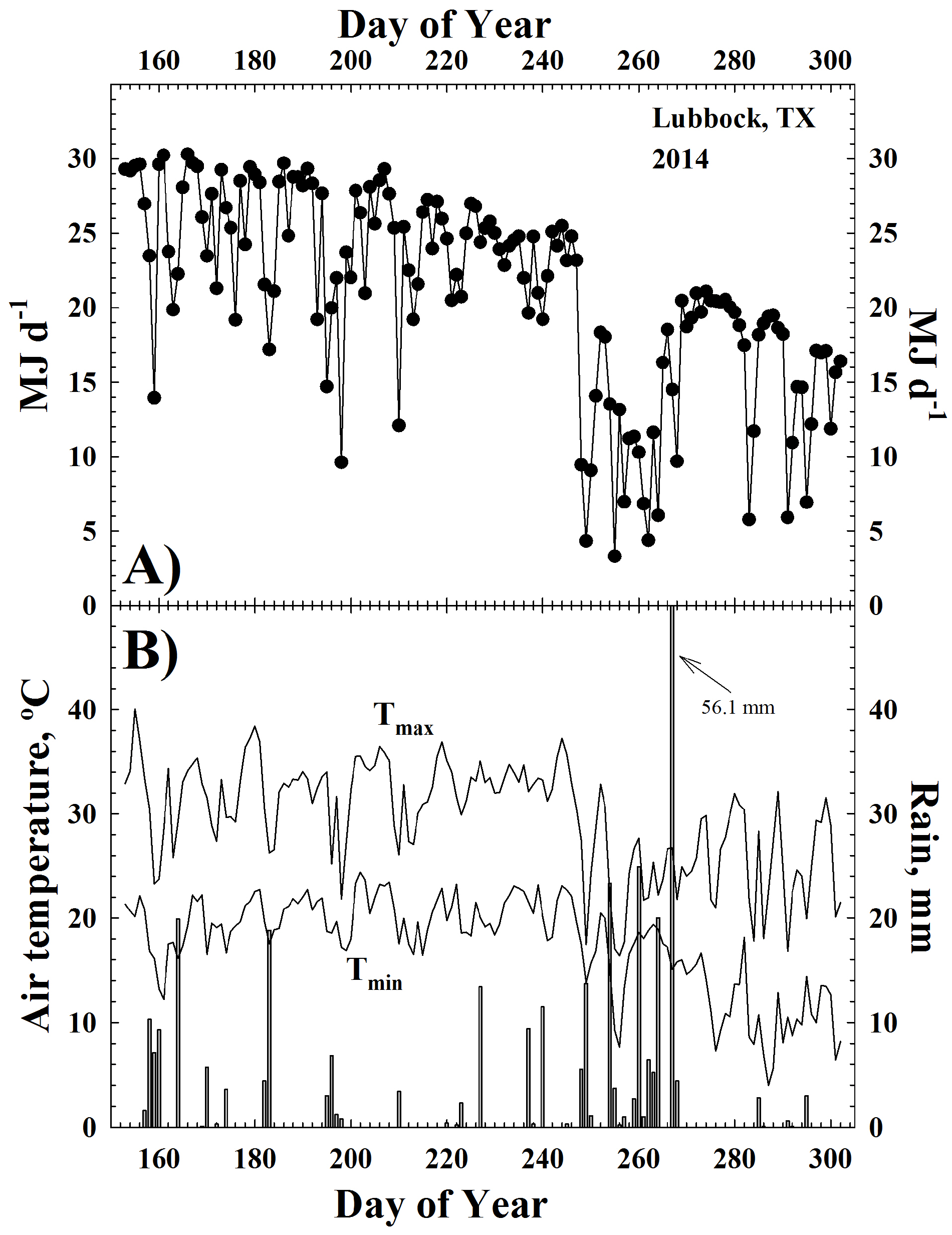
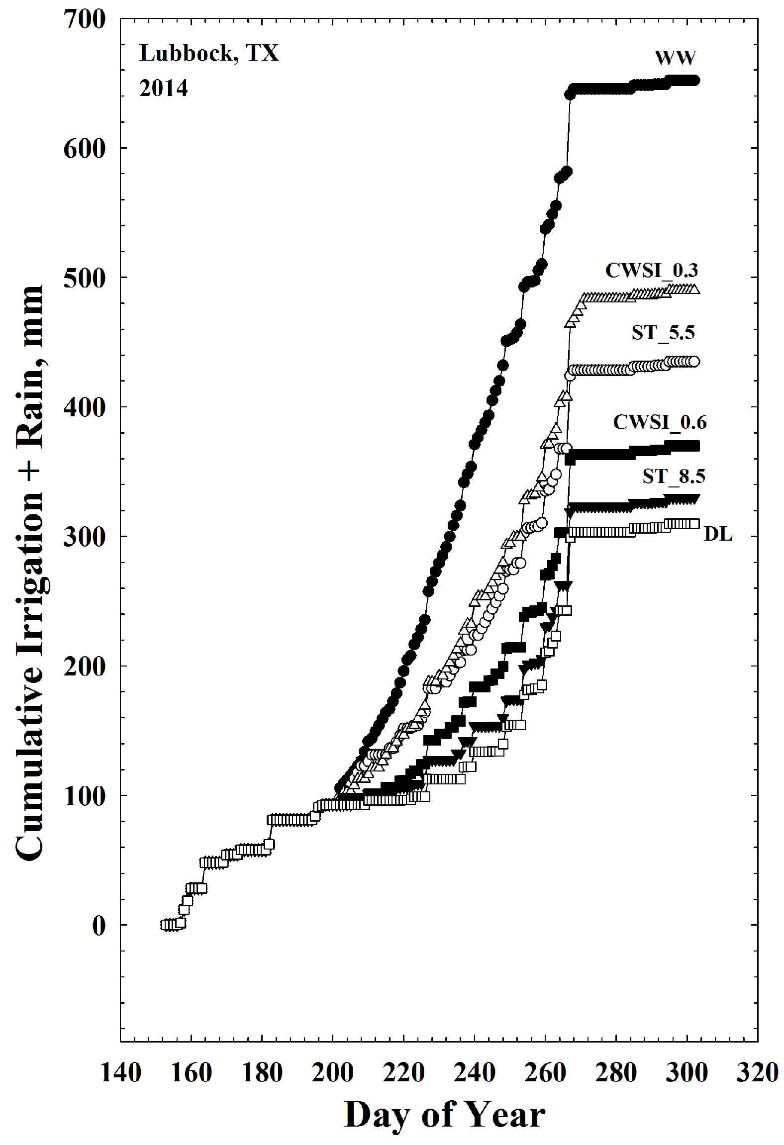
Weather in 2014 was characterized by an unusual overcast and rainy period from about DOY 248–268 (5–25 September) with an especially intense rainfall of 56 mm on DOY 267 (Figure 1). Total rainfall over the course of the season (June–October) was 310 mm, which is only slightly above the 30-year average of 287 mm for Lubbock, TX, USA [25]. The six water treatments resulted in a wide range of cumulative irrigation plus rainfall (Figure 2) and an estimated crop water use ranging from about 353 mm in the DL treatment to about 625 mm in the WW treatment (Table 1).

Figure 1. (A). Total solar irradiance vs. day of year; (B). Maximum (Tmax) and minimum (Tmin) air temperature vs. day of year. Histograms on the x-axis indicate rainfall events and amounts on the right side y-axis.

Figure 1. (A). Total solar irradiance vs. day of year; (B). Maximum (Tmax) and minimum (Tmin) air temperature vs. day of year. Histograms on the x-axis indicate rainfall events and amounts on the right side y-axis.

Figure 2. Seasonal trends in irrigation + rainfall for six water treatments: well-watered (WW), Stress Time (ST), 5.5 h (ST_5.5), Stress Time, 8.5 h (ST_8.5), Crop Water Stress Index 0.3 (CWSI_0.3), Crop Water Stress Index 0.6 (CWSI_0.6), and Dry Land (DL).

Figure 2. Seasonal trends in irrigation + rainfall for six water treatments: well-watered (WW), Stress Time (ST), 5.5 h (ST_5.5), Stress Time, 8.5 h (ST_8.5), Crop Water Stress Index 0.3 (CWSI_0.3), Crop Water Stress Index 0.6 (CWSI_0.6), and Dry Land (DL).

Table 1. Lint quality characteristics and seasonal crop water use for six different water treatments. Means within the same column followed by the same letter are not significantly different at p ≤ 0.05.

Water Treatment	Micronaire Value	Length	Strength	Water Used
	μg/inch	mm	g/tex	mm
WW	3.1 B	30.3 A	28.2 AB	625
ST_5.5	4.6 A	28.9 B	31.0 A	439
ST_8.5	4.7 A	26.6 C	26.9 B	367
CWSI_0.3	4.4 A	29.1 AB	29.1 AB	494
CWSI_0.6	4.8 A	28.3 B	29.5 AB	386
DL	4.8 A	25.2 C	23.1 C	353

Table 1. Lint quality characteristics and seasonal crop water use for six different water treatments. Means within the same column followed by the same letter are not significantly different at p ≤ 0.05.

Water Treatment	Micronaire Value	Length	Strength	Water Used
	μg/inch	mm	g/tex	mm
WW	3.1 B	30.3 A	28.2 AB	625
ST_5.5	4.6 A	28.9 B	31.0 A	439
ST_8.5	4.7 A	26.6 C	26.9 B	367
CWSI_0.3	4.4 A	29.1 AB	29.1 AB	494
CWSI_0.6	4.8 A	28.3 B	29.5 AB	386
DL	4.8 A	25.2 C	23.1 C	353

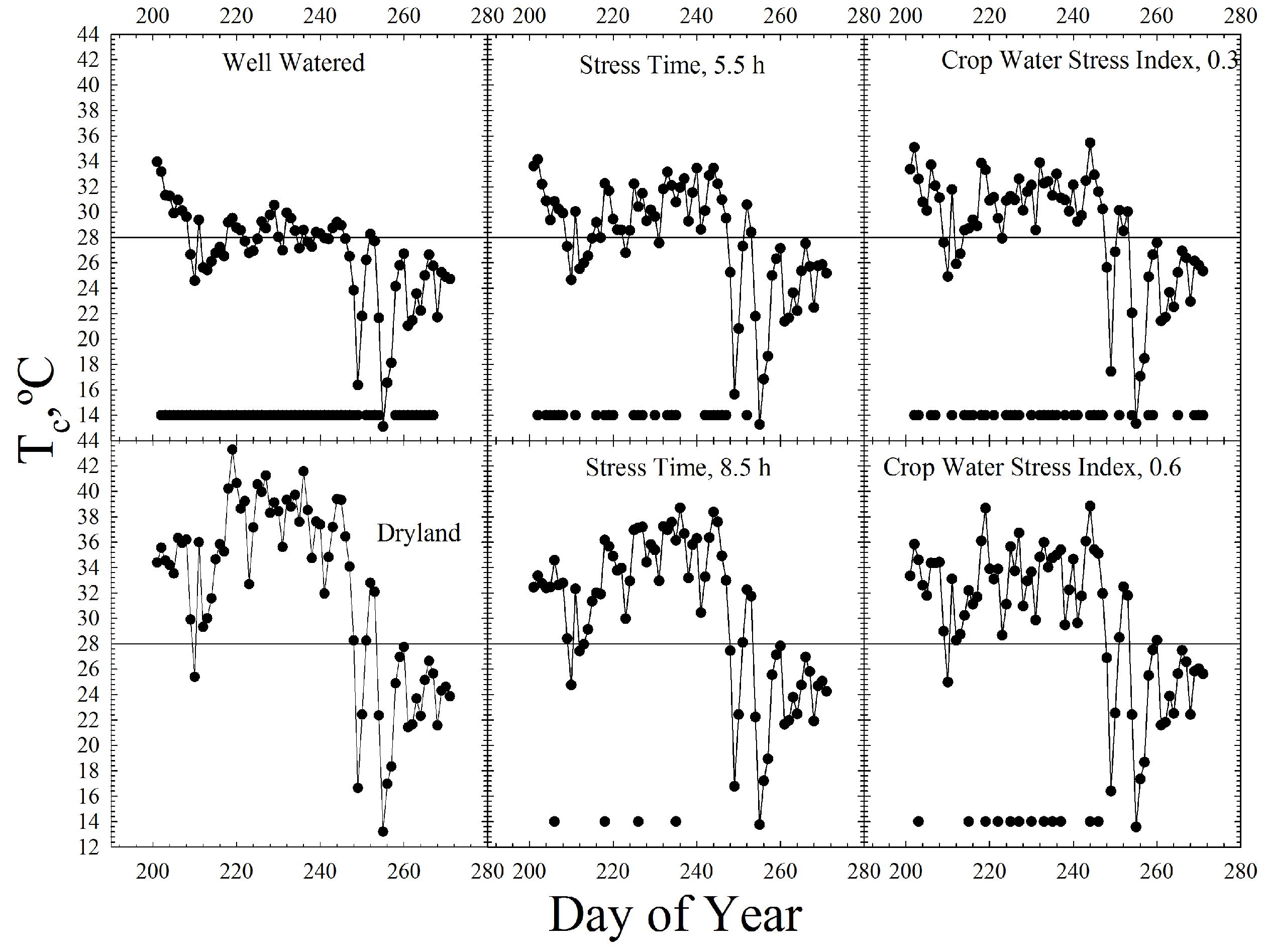
Shown in Figure 3 are T_c vs. DOY averaged over 12.00 to 15.00 h for all six water treatments. Horizontal lines in Figure 3 at 28 °C are drawn in each panel to correspond with the temperature threshold used by the ST treatments. Filled circles across the bottoms of the panels represent days when irrigation events occurred. In general, treatments receiving more water had cooler T_c as especially evident in the comparison of the WW and DL treatments (Figure 3). Interestingly, the ST_8.5 treatment only triggered 4 irrigation events throughout the growing season. This likely happened due to the water saturated water profile at the beginning of the season and the cool and wet period (DOY 248–268) noted above. As expected, the CWSI_0.3 irrigated more frequently and had cooler T_c compared to the CWSI_0.6 treatment (Figure 3).

Figure 3. Average midday (12.00 to 15.00 h) canopy temperatures (T_c, °C) for six water treatments vs. day of year. Vertical line, drawn for comparison across treatments, at 28 °C indicates the canopy temperature threshold for the ST_5.5 and ST_8.5 treatments, respectively. Filled circle symbols in each panel indicated days when a 5 mm irrigation event was triggered. Irrigation amounts in the well watered (WW) represent 110% of calculated potential evapotranspiration during the previous time interval. The dryland (DL) treatment received no irrigation.

Figure 3. Average midday (12.00 to 15.00 h) canopy temperatures (T_c, °C) for six water treatments vs. day of year. Vertical line, drawn for comparison across treatments, at 28 °C indicates the canopy temperature threshold for the ST_5.5 and ST_8.5 treatments, respectively. Filled circle symbols in each panel indicated days when a 5 mm irrigation event was triggered. Irrigation amounts in the well watered (WW) represent 110% of calculated potential evapotranspiration during the previous time interval. The dryland (DL) treatment received no irrigation.

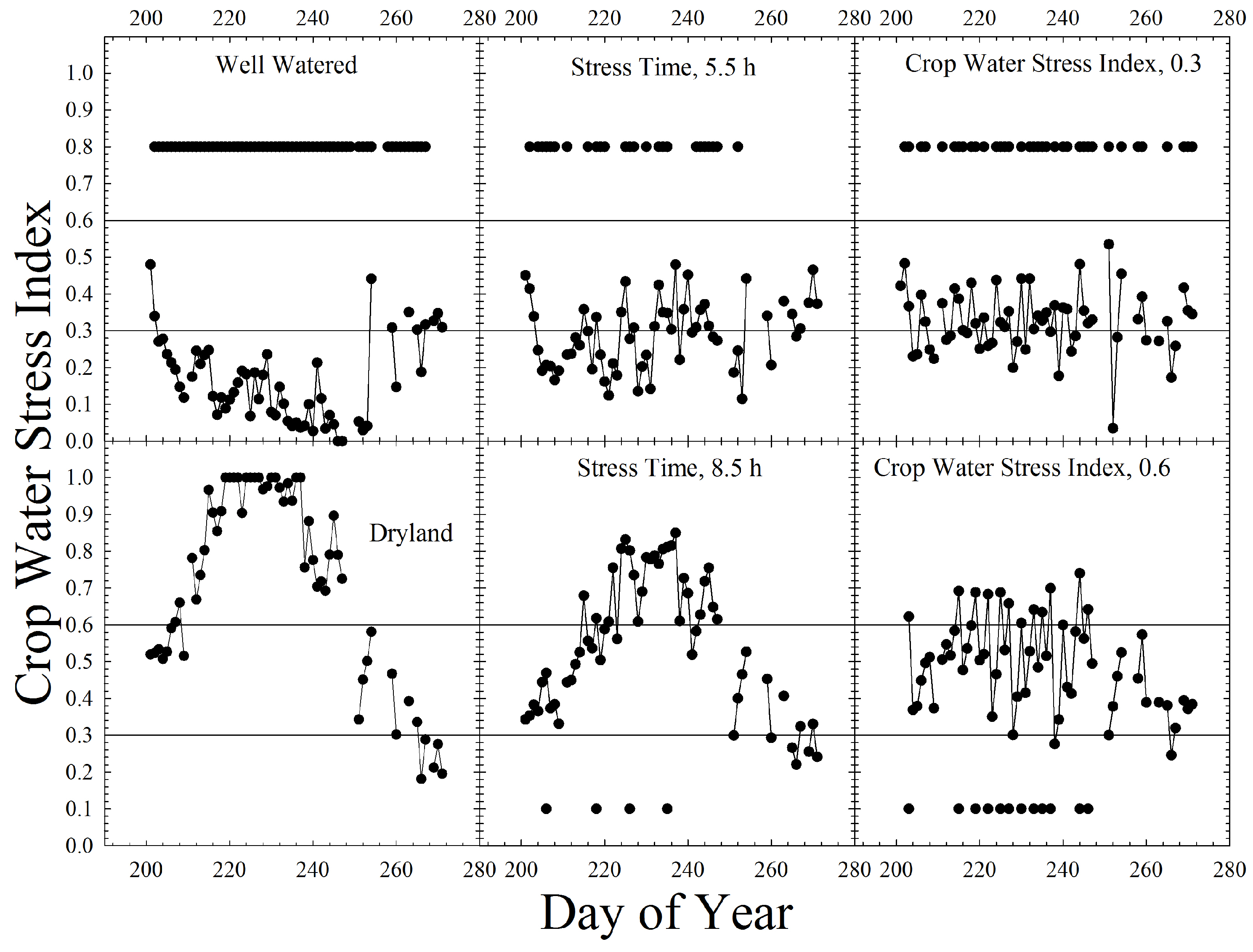
Figure 4 shows calculated CWSI values vs. DOY averaged from 12.00 to 15.00 h for all six water treatments. Horizontal lines are drawn at y-axis of 0.3 and 0.6 to illustrate the CWSI trigger points for the CWSI_0.3 and CWSI_0.6 treatments. Again filled circles indicated irrigation events also shown in Figure 3. As expected, mid-season CWSI values approached 0.0 and 1.0 for the WW and DL treatments, respectively (Figure 4). The steadily increasing CWSI calculations for the ST_8.5 treatment over the range from about DOY 200 to 240 indicated a steadily increasing amount or degree of crop drought stress. The CWSI values cycled around their respective irrigation trigger set points of 0.3 and 0.6 for the CWSI_0.3 and CWSI_0.6, respectively as was intended (Figure 4).

Figure 4. Average midday (12.00 to 15.00 h) Crop Water Stress Index calculations for six water treatments vs. day of year. Vertical lines, drawn for comparison across treatments, at 0.3 and 0.6 indicate Crop Water Stress Index thresholds for triggering an irrigation event in the CWSI_0.3 and CWSI_0.6 treatments, respectively. Filled circle symbols at the bottom or top of the panels indicate days when irrigation was triggered. For the Stress Time and the Crop Water Stress Index treatments, 5 mm of water was applied at each irrigation event. Irrigation amounts in the well watered (WW) represent 110% of calculated potential evapotranspiration during the previous time interval. The dryland treatment (DL) received no irrigations.

Figure 4. Average midday (12.00 to 15.00 h) Crop Water Stress Index calculations for six water treatments vs. day of year. Vertical lines, drawn for comparison across treatments, at 0.3 and 0.6 indicate Crop Water Stress Index thresholds for triggering an irrigation event in the CWSI_0.3 and CWSI_0.6 treatments, respectively. Filled circle symbols at the bottom or top of the panels indicate days when irrigation was triggered. For the Stress Time and the Crop Water Stress Index treatments, 5 mm of water was applied at each irrigation event. Irrigation amounts in the well watered (WW) represent 110% of calculated potential evapotranspiration during the previous time interval. The dryland treatment (DL) received no irrigations.

These six water treatments resulted in a wide range of crop water use and this had significant effects on cotton fiber quality characteristics (Table 1). Micronaire, and fiber length and strength are important lint quality characteristics that determine, in part, the value of a farmer’s cotton harvest. Micronaire value was significantly reduced with greater crop water use in the WW treatment compared with the other five water treatments. In an opposite trend, both fiber length and strength were reduced with decreasing crop water use (Table 1).

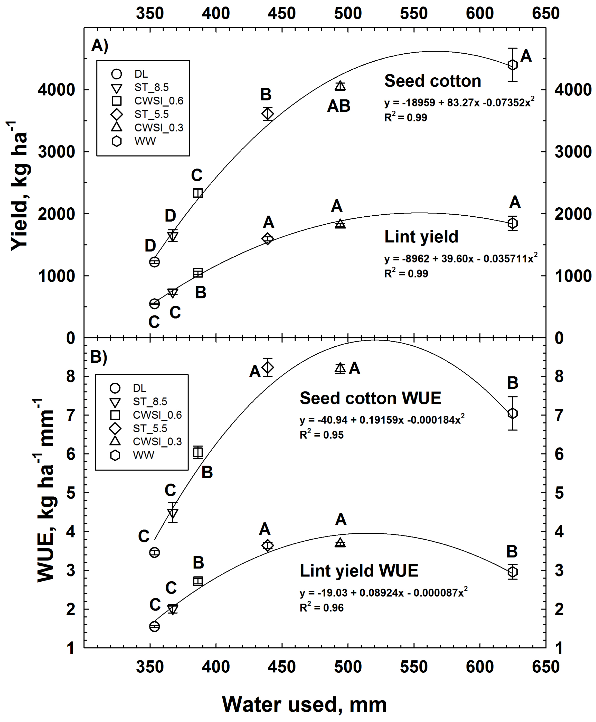
Both seed cotton and lint yields increased with increasing crop water use up to about 439 to 494 mm (Figure 5a) followed by a general leveling off of yield up to the WW treatment. In cotton, yield depends on the production and retention of bolls and both can be decreased by drought [26]. In some cases, over watering cotton can lead to reduced yield [27,28]. Cotton is an indeterminate crop that can grow vegetatively and reproductively simultaneously. This allows cotton to dynamically adjust fruit load in response to stress such as drought. In contrast, for determinant cereal crops the timing and severity of drought stress is critical since drought stress at reproductive developmental growth stages can severely reduce grain yields compared to a drought stress at the vegetative stage of growth [29]. Indeed, grain sorghum yield was found to be far more sensitive to CWSI values than was cotton lint yield [30].

Figure 5. (A) Seed cotton and lint yield vs. seasonal water use; (B) Seed cotton and lint yield water use efficiency (WUE) vs. seasonal water use. Vertical bars on each data point are ± SE. Letters near data symbols indicate mean separation at p ≤ 0.05.

Figure 5. (A) Seed cotton and lint yield vs. seasonal water use; (B) Seed cotton and lint yield water use efficiency (WUE) vs. seasonal water use. Vertical bars on each data point are ± SE. Letters near data symbols indicate mean separation at p ≤ 0.05.

In this experiment, cotton WUE for both seed cotton and lint yield peaked at crop water use of about 439 (ST_5.5) to 494 mm (CWSI_0.3) and declined slightly but significantly at 625 mm (WW) (Figure 5b). This finding may not be especially robust with respect to different years, locations or cultivars. Zwart and Bastiaanssen [31] reviewed 16 studies on cotton water use efficiency (e.g., their crop water productivity, CWP) and concluded yield per water use functions were valid only locally and cannot be used in macro-scale planning of agricultural water management. They found a major climatic factor influencing WUE was vapor pressure deficit, which tended to decrease as latitude increases. In an extensive review of the literature Grismer [32] reported that cotton seed and/or lint WUE is affected by a wide range of factors including tillage, planting patterns, soil salinity and irrigation methods and timing. Strong interactions among cultivar, year and irrigation rates found by Snowden et al. [33] indicated that selecting the appropriate cultivar and irrigation regime without foreknowledge of the upcoming seasonal weather pattern is currently difficult.

The results reported in this paper and also critically in our review of the literature, indicate that optimizing WUE is difficult because WUE is dependent on cotton cultivar, location and years. Thus, the better of these two different irrigation methods (e.g., ST vs. CWSI) and even the best irrigation trigger set points among these two methods will likely vary with environment. The most obvious example of this is simply a wet vs. dry year at a single location.

4. Conclusions

We concluded that WUE may be optimized in irrigated cotton with less water than that required for maximum lint yield. Improvements in long-range weather forecasting may allow cotton agronomists of the future to fine-tune irrigation scheduling and cultivar selection for a particular location in order to maximize WUE while saving water resources.