Towards Remote Estimation of Radiation Use Efficiency in Maize Using UAV-Based Low-Cost Camera Imagery

Abstract

Radiation Use Efficiency (RUE) defines the productivity with which absorbed photosynthetically active radiation (APAR) is converted to plant biomass. Readily used in crop growth models to predict dry matter accumulation, RUE is commonly determined by elaborate static sensor measurements in the field. Different definitions are used, based on total absorbed PAR (RUE_total) or PAR absorbed by the photosynthetically active leaf tissue only (RUE_green). Previous studies have shown that the fraction of PAR absorbed (fAPAR), which supports the assessment of RUE, can be reliably estimated via remote sensing (RS), but unfortunately at spatial resolutions too coarse for experimental agriculture. UAV-based RS offers the possibility to cover plant reflectance at very high spatial and temporal resolution, possibly covering several experimental plots in little time. We investigated if (a) UAV-based low-cost camera imagery allowed estimating RUEs in different experimental plots where maize was cultivated in the growing season of 2016, (b) those values were different from the ones previously reported in literature and (c) there was a difference between RUE_total and RUE_green. We determined fractional cover and canopy reflectance based on the RS imagery. Our study found that RUE_total ranges between 4.05 and 4.59, and RUE_green between 4.11 and 4.65. These values are higher than those published in other research articles, but not outside the range of plausibility. The difference between RUE_total and RUE_green was minimal, possibly due to prolonged canopy greenness induced by the stay-green trait of the cultivar grown. The procedure presented here makes time-consuming APAR measurements for determining RUE especially in large experiments superfluous.

1. Introduction

In agronomy, radiation-use efficiency (RUE, also referred to as light use efficiency LUE) is defined as crop biomass produced per unit of total solar radiation or photosynthetically active radiation (PAR) intercepted by the canopy [1]. It follows the concept introduced decades ago [2], where the amount of photosynthates or dry biomass production (DM in g m⁻²) is expressed as the product of the fraction of absorbed photosynthetically active radiation (fAPAR, with APAR defined as absorbed solar radiation between 400 and 700 nm wavelength in MJ m⁻²) and the efficiency (ε) with which the absorbed light is converted into fixed carbon (Equation (1)).

$$\mathrm{DM}=\mathrm{fAPAR}\times \mathrm{PAR}\times \mathsf{\epsilon }$$

(1)

This concept is widely used in dynamic crop growth modelling [1], where daily biomass production is estimated as the product of the amount of radiation intercepted and the RUE for forecasting crop growth and yield. The model’s estimation accuracy is affected by limitations of the model itself, because factors influencing biomass production are not considered by the model, and when model parameters or input variables, such as cultivar-dependent RUE, are not available [3]. Commonly, a constant RUE value is assumed, determined by elaborate field measurements. Unfortunately, there is no standardized procedure to estimate RUE, which has led to various units and experimental approaches [4]. Gitelson and Gamon [5] point out that there are at least three widely used definitions of photosynthetic RUE based on

• incoming radiation (RUE_inc) calculated as

  $${\mathrm{RUE}}_{\mathrm{inc}}=\mathrm{DM}/{\mathrm{PAR}}_{\mathrm{inc}}$$

  (2)

  with PAR_inc = incident PAR and DM = dry matter produced,
• total absorbed light (RUE_total), calculated as

  $${\mathrm{RUE}}_{\mathrm{total}}=\mathrm{DM}/\left(\mathrm{fAPAR}\times {\mathrm{PAR}}_{\mathrm{inc}}\right)$$

  (3)

  with fAPAR as the fraction of daily PAR absorbed, and
• radiation absorbed by photosynthetically active vegetation (RUE_green), calculated as

  $${\mathrm{RUE}}_{\mathrm{green}}=\frac{\mathrm{DM}}{{\mathrm{fAPAR}}_{\mathrm{green}}}\times {\mathrm{PAR}}_{\mathrm{inc}}$$

  (4)

  with fAPAR_green calculated as

  $${\mathrm{fAPAR}}_{\mathrm{green}}=\mathrm{fAPAR}\times (\frac{\mathrm{greenLAI}}{\mathrm{totalLAI}})$$

  (5)

where green leaf area index (gLAI) describes the photosynthetically functional leaf tissue per unit ground area, and total LAI the combination of both green and senesced (i.e., brown) leaf area per unit ground area. The authors furthermore argue that the estimation of crop productivity could be different if different RUE definitions are used, and so they recommend considering RUE_green as the standard RUE definition, since it is not confounded by changing pigment and green canopy structure during plant growth and senescence [5]. During the vegetative stage, when LAI_green is equal to total LAI, fAPAR_green represents the fraction of absorbed photosynthetically active radiation used for photosynthesis. However, during the reproductive stage and subsequent senescence, fAPAR_total becomes insensitive to decreasing crop greenness since both, photosynthetic and non-photosynthetic components, intercept PAR_inc, while progressively less is used for photosynthesis. Therefore, to obtain a measure of the fAPAR absorbed solely by the photosynthetic component of the vegetation, the fraction of radiation absorbed by photosynthetically active green vegetation (fAPAR_green) is calculated [6].

The most widely used method to calculate RUE is to fit a linear relationship between cumulative biomass accumulation and cumulative radiation interception, with the slope of the linear relationship representing the RUE [4]. The determination of RUE_inc and RUE_total in the field requires the measurement of intercepted or absorbed radiation and dry biomass at time intervals that are adequate for accurate estimations of both [1]. The determination of RUE_green requires additional measurements of green LAI and brown LAI (i.e., senesced material). Dry biomass used in the calculation usually comprises net aboveground biomass, but not root mass [4]. Absorbed PAR (APAR) is commonly derived as:

$$\mathrm{APAR}={\mathrm{PAR}}_{\mathrm{inc}}-{\mathrm{PAR}}_{\mathrm{out}}-{\mathrm{PAR}}_{\mathrm{trans}}+{\mathrm{PAR}}_{\mathrm{soil}}$$

(6)

with PAR_inc representing the incoming PAR radiation above the canopy, PAR_out the PAR radiation reflected by canopy and soil, PAR_trans the PAR radiation transmitted through the canopy and PAR_soil the PAR radiation reflected by the soil (and subsequently absorbed by plant tissue). PAR_inc is measured by a sensor above the canopy, pointing towards the sky, PAR_out with a sensor pointing downwards towards the canopy. PAR_trans is tracked with a sensor placed just above the ground underneath the canopy looking upward, and PAR_soil with a sensor placed a few centimeters above the ground, looking downward (e.g., done by [6,7,8]).

RUE can be affected by environmental factors such as temperature, radiation and air humidity, or by plant factors such as nutritional and water status, plant development, and source-sink regulation [1]. It is therefore critical that estimates of crop growth and RUE are obtained under optimal growth conditions [7]. A range of potential maize (Zea mays L.) RUE values have been reported in the literature (see

Table 1. List of maximum radiation use efficiency (RUE) values reported for maize.

Source	Average RUE	Based on	Location	Comments
[7]	3.8 g MJ−1	APAR	Sterling, NE, and Lincoln NE, USA	Near-optimal growth conditions, five growing seasons, irrigated
[6]	2.24 gC MJ−1	APARgreen	Mead, NE, USA	Multiyear observations, irrigated and rainfed, high variability within maize cultivars
[12]	3.35 g MJ−1	IPAR	Ames, IA, USA	One growing season, rainfed
[4]	1.6 g MJ−1 during vegetative growth, 1.7 g MJ−1 during reproductive growth	Solar radiation	Various	Review of publications from different locations with different measurement techniques
[13]	3.3 g MJ−1	APAR	Toulouse, France	Three growing seasons, irrigated
[14]	3.41 g MJ−1	APAR	Southern Ontario, Canada	One growing season, rainfed, nitrogen/no nitrogen treatment

Factors for conversion to total solar radiation basis: 0.5 for IPAR, 0.425 for APAR [4].

for a list), with most values ranging between 3.3 g MJ⁻¹ and 3.8 g MJ⁻¹.

The overall RUE of a maize crop throughout the growing season strongly depends on the duration of greenness of plant tissue. Recently, the stay green (SG) trait has been identified as an important component in the genetic improvement of several crops to promote stress tolerance and yield improvement [9]. In maize, this is associated with delayed canopy senescence compared to standard genotypes, which implies a longer period of photosynthetic activity and a longer N retention in the leaves during grain filling, but also lower kernel N concentrations, which might result in lower grain yield [10]. Swanckaert et al. [11] found, however, that the stay green trait does not necessarily provoke higher assimilate accumulation in the leaves, but is rather a cosmetic one [11].

Remote sensing offers potential to reliably estimate the fraction of incoming PAR absorbed by active tissue in the canopy, even across larger areas. This is based on the premise that surface structural and optical properties are governed by the vegetation fraction and leaf area index. The interlink is established either via relating fAPAR to spectral vegetation indices (SVI) or via the usage of radiation transfer models [15]. In mixed pixels containing different land covers, precise land cover estimation through remote sensing is challenging. The SVI-fAPAR model is commonly chosen where the spectral reflectance is a linear combination of values of background soil and vegetation [16].

UAV-based remote sensing offers coverage at unpreceded spatial and temporal resolutions due to the low flying altitudes and the versatile, flexible employment of the platform possibly independent from irradiation conditions. UAV-based applications in agronomy comprise biomass estimation via plant height measurements [17,18], LAI estimation [19,20], analysis of phenology [21] and yield prediction [22,23,24], amongst others.

Well-calibrated UAV-based spectral imagery provides reflectance information at much greater detail than other sensors, which reduces the amount of mixed pixels combining soil and vegetation information. This could be used to draw conclusion on the light absorption ability of crop canopies over the course of the growing season, especially within small-scale experimental plots. Furthermore, the spatial resolution allows for the separation of plant tissue, soil and other features in the field.

Based on these findings, we asked:

• Does UAV-based commercial off-the-shelf (COTS) digital camera imagery reflectance data allow for fAPAR estimation support, for ultimately determining RUEs of maize in small-scale experimental plots of variable LAI and biomass development (measured destructively)?
• Do RUE values of maize derived from this technique differ substantially from field-collected ones reported in the literature?
• Is there a difference between RUE_total and RUE_green in the treatments?

We are not aware of any study that partly estimates fAPAR for RUE determination from UAV-based low-cost camera imagery.

2. Material and Methods

2.1. Study Site and Field Experiment

The field experiment was established in 2016 at Campus Klein-Altendorf (CKA), University of Bonn’s own agricultural research facility located southwest the city of Bonn, Germany (6°59′32″ E, 50°37′51″ N, 184 m above sea level). Climate is characterized by temperate humid conditions with maritime influence. Long-term average precipitation is 625 mm; average temperature is 9.6 °C. The soil is classified as alkaline, nutrient-rich Haplic Luvisol that developed from Loess [25,26].

The sole purpose of this experiment was to expand plant productivity by formation of different leaf areas; variability in biomass thus resulted from different light absorption over time. Our assumption was to thereby improve the general statement of this study, which could represent heterogeneous growth in a common field. It was not our intention to investigate the influence of management on biomass accumulation.

Established in a random sampling design, the experiment consisted of a combination of two plant densities (PD) and two treatments of nitrogen (N). The plant densities comprised 50,000 plants ha⁻¹ and 100,000 plants ha⁻¹, the nitrogen treatments 100 kg ha⁻¹ and 200 kg ha⁻¹, respectively. Every treatment was conducted on a plot sized 3 × 30 m, with 5 repetitions each. Row spacing was 0.75 m (i.e., 4 rows per plot). Nitrogen was applied as inorganic ammonium sulphate (ASN) before planting as one-time treatment. Pesticides were applied according to standard practices, and no irrigation scheme was practiced. All treatments were checked for wrongly set plants. Low plant density plots were manually thinned out after emergence.

Rainfall, air temperature at 2 m aboveground and incoming global solar radiation were recorded at the research station’s weather station (GWU-Umwelttechnik GmbH, Erftstadt, Germany) in the vicinity of the field.

The hybrid cultivar Ricardinio (KWS Saaten AG, Einbeck, Germany) with stay-green characteristics was grown, which has a recommended plant density, according to the seed producer, of 90,000–95,000 plants ha⁻¹ in non-water limited environments (see

Table 2. Basic data of the trial.

BBCH Stage	Date	Temperature Sum [°Cd]
Planting Date	4 May 2016	-
Emergence	10 May 2016	44.45
Begin Flowering	15 July 2016	585.72
Fruit Development: Milk-ripe stage	15 August 2016	918.41
Full ripening	23 September 2016	1346.67
Harvest	29 October 2016	1454.2

for further information, including captured phenological stages according to BBCH scale). The temperature sum was calculated using 8 °C as base temperature as confirmed for temperate climates by Birch et al. [27]. Temperatures beyond 30 °C were included in the calculation as the maximum temperature of 30 °C, since no increased growth was observed beyond that temperature. A total sum of 353.1 mm of precipitation was recorded between planting and harvest. The recorded long-term average (1956–2017) precipitation from May to October is 361 mm (www.cka.uni-bonn.de, accessed on 15 January 2018).

2.2. Leaf Area Index and Dry Biomass Measurements

For measuring leaf area index, 0.5 m of plants in two adjacent rows were sampled destructively at two positions within 4 plots of each treatment at every sampling date (i.e., 4 treatments × 4 plots × 2 samples = 32 samples per sampling date). To minimize edge effects, we did not sample the outer rows of each plot and skipped 0.5 m of standing plants between the collection dates. Four plots (i.e., one plot per treatment) remained unsampled during the entire course of the trial. Samples were immediately transported back to the institute and split into green and senescent material by visual assessment. Green and senescent leaf area was measured separately using the LI-COR LI-3100C area meter (LI-COR Inc., Lincoln, NE, USA). gLAI and brown LAI respectively, was determined by dividing the leaf area of each sample by the sampling area (i.e., leaf area/0.75 m²). Samples were taken on ten dates in 2016, with an interval of roughly 14 days. Assessing leaf area by destructive sampling is considered the most accurate method and often serves as calibration for indirect measurement techniques [28].

Aboveground biomass was measured from the same samples taken for leaf area measurements. Samples were oven-dried at 105 °C for at least 48 h until constant weight and weighed subsequently.

2.3. Collection of Spectral Data and Preprocessing

Spectral data was collected using two Canon ELPH 110 HS digital compact red-green-blue (RGB) cameras, modified by LDP LLC Inc. (Carlstad, NJ, USA). The cameras 1 2/3 inch sized CMOS sensor comprised 4608 × 3456 recording pixels (i.e., 16.1 Megapixels). The first camera (hereafter: RGNIR camera) was fitted a blue rejection filter, with sensitivity in the red, green and near-infrared (NIR) domain from roughly 800–900 nm. The information in the blue band was replaced by information in the NIR domain. The second camera (hereafter: BGNIR camera) was fitted with a dual-band-pass filter that blocks light in the red domain; this rendered the sensor sensitive for NIR light in the wavelengths 680 nm to 780 nm. The RGNIR camera delivered R = Red + NIR, G = Green + NIR and B = NIR only, the BGNIR camera delivered B = Blue + NIR, G = Green and R = NIR.

The cameras were mounted inside a frame underneath a Mikrokopter OktoXL6S12 (HiSystems GmbH, Moormerland, Germany) octocopter. Data was collected around noon to avoid shadow cast, on mostly cloud-free days, immediately before the sampling of the plants. Images were acquired from an altitude of 50 m (~ground sampling distance of 1.5 cm) at nadir view, with a focal length of 4.3 mm and a variable shutter speed that was adjusted from one campaign to the next, depending on incident light conditions. Three differently grey-scaled reference targets placed next to the field served for the conversion to reflectance values (with nominal reflections of ~4%, ~16% and ~58% of light).

Images captured in RAW format were subsequently corrected for lens barrel distortion, vignetting effects [21,29] and NIR band interference before being converted to reflectance values using the empirical line calibration method [30]. Orthomosaics were created using Agisoft Photoscan Professional (Agisoft LLC, St. Petersburg, Russia).

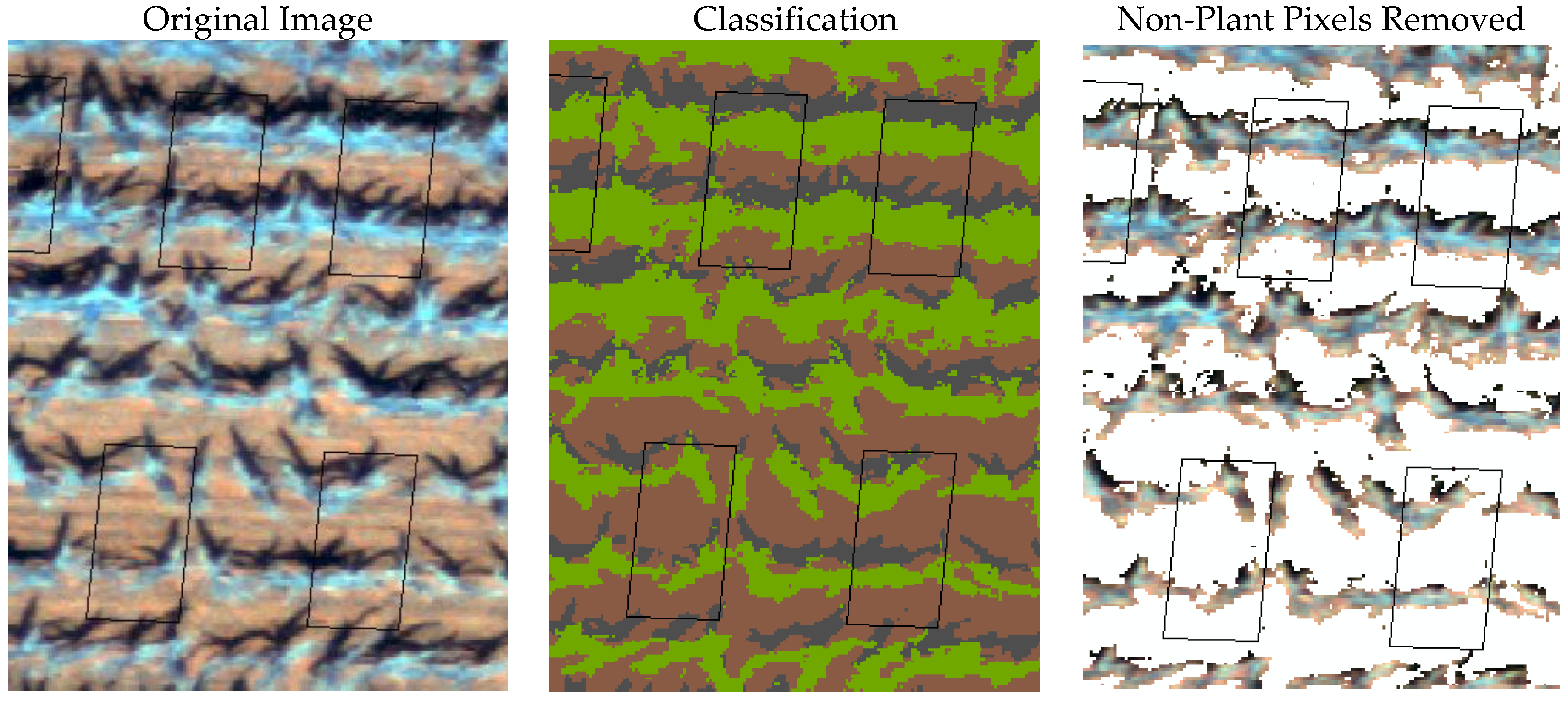
2.4. Image Classification and Estimation of Fractional Cover

We classified each orthomosaic into the components plant tissue, illuminated soil and shaded soil (cast from plants) using the supervised random forest (RF) classifier implemented in R’s [31] RStoolbox [32]. RF is a powerful classifier and widely used in RS applications based on multispectral and hyperspectral data [33,34].

We estimated fractional cover (fCover, i.e., the area of each sampling plot covered by plant material in relation to the entire plot area) to relate reflectance of plant tissue to the gap fraction that would be measured by static sensors in the field. To do this, we divided the number of pixels classified as plant tissue within each sampling plot by the number of total pixels (comprising plant tissue, illuminated soil and shaded soil).

For removal of non-plant reflectances, the classes ‘illuminated soil’ and ‘shaded soil’ were subsequently masked and pixel values were replaced with missing values. Pixel values of plant tissue were extracted and averaged within exactly the same ground area of the field where each sample was taken, using the raster [35] package implemented in R [31]. NA values were ignored in the calculation.

Figure 1 shows the example of an original image, the classification and the image after removal of soil pixels.

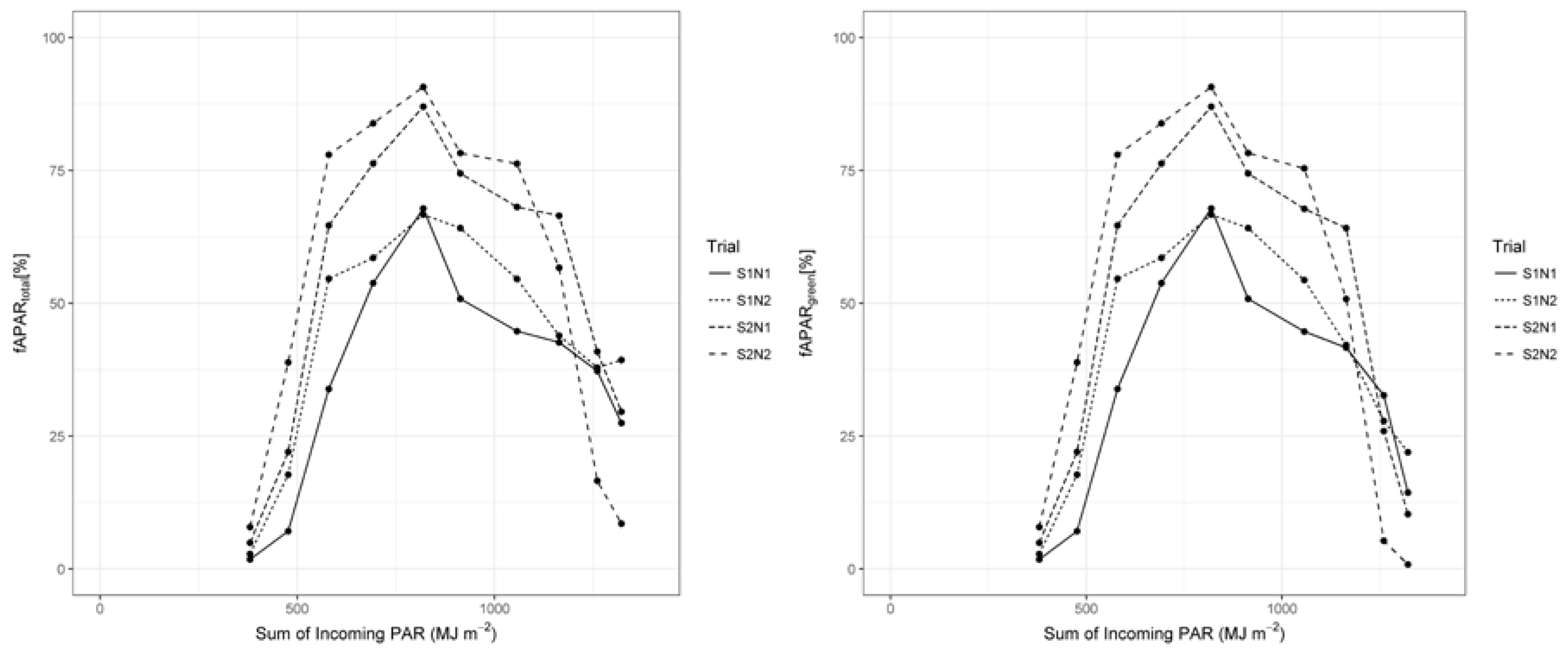
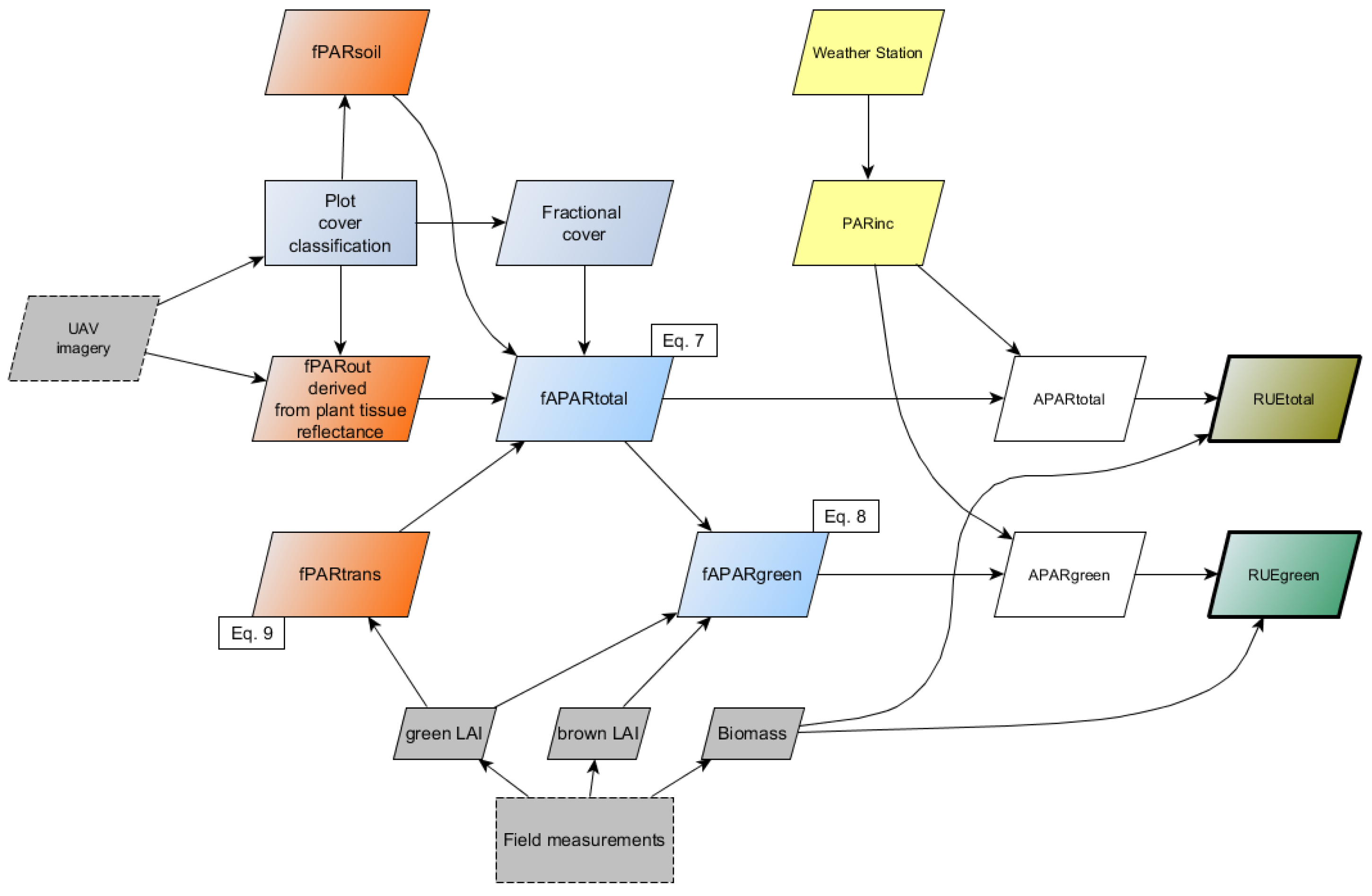
2.5. Derivation of fAPAR and APAR

fAPAR_total and fAPAR_green were calculated as shown in Equations (7) and (8). fPAR_out describes the fraction of incoming PAR (PAR_inc) that was reflected by the canopy, fPAR_trans the fraction of PAR_inc that was transmitted through the canopy. fPAR_soil is the fraction of PAR transmitted through the canopy that was reflected by the soil. fCover describes the fractional vegetation cover in each sampling plot.

$${\mathrm{fAPAR}}_{\mathrm{total}}=\left(100\%-{\mathrm{fPAR}}_{\mathrm{out}}-{\mathrm{fPAR}}_{\mathrm{trans}}+{\mathrm{fPAR}}_{\mathrm{soil}}\right)\times \mathrm{fCover}$$

(7)

$${\mathrm{fAPAR}}_{\mathrm{green}}={\mathrm{fAPAR}}_{\mathrm{total}}\times (\frac{\mathrm{gLAI}}{\mathrm{totalLAI}})$$

(8)

In order to derive RUE based on UAV-based low cost imagery, we assumed the following:

• The spectrum captured by the blue, red and green bands of the cameras corresponded roughly to the spectrum of photosynthetically active radiation (PAR, 400–700 nm).
• PAR_inc (derived as 0.5× total solar radiation) measured by the weather station corresponded to PAR_inc above the canopy in the field.
• fPAR_out corresponded to the average reflectance value (%) of plant tissue that was derived from the red, green and blue bands of the converted camera imagery.
• fPAR_trans was not measured directly. We estimated the fraction of PAR transmitted through the canopy by applying the Lambert–Beer law Equation (9), where k is the extinction coefficient and gLAI the green leaf area index:

  $${\mathrm{fPAR}}_{\mathrm{trans}}={\mathrm{e}}^{-k\times \mathrm{gLAI}}$$

  (9)

  A number of k values have been reported for maize, with recent publications suggesting a range between 0.49 [7], 0.63 [36] and 0.65 [37] for maize hybrid plants. We selected a k value of 0.55 for our analysis.
• fPAR_soil reflects a fixed amount of fPAR_trans back into the direction of the canopy, where it is absorbed by the plants. We averaged all pixel values in the class ‘illuminated soil’, thereby neglecting those influences that vary soil moisture levels and so affect soil reflectance. An average reflectance of 10% was assumed, based on the average of soil reflectance within the class ‘illuminated soil’.
• Temporal increase in fAPAR between sampling dates follows a linear relationship.
• The plants grew free from environmental stresses.

2.6. Calculation of RUE

RUE was derived using the cumulative biomass and APAR method, since the majority of studies relies on this method. The amount of PAR that was absorbed by the plants was derived for each sampling date by calculating the definite integral in the plot of cumulated PAR over the growing season vs. fAPAR_total and fAPAR_green, respectively. This value was plotted against destructively-measured dry biomass; the slope of the linear regression indicated the RUE.

The entire workflow is illustrated in Figure 2.

3. Results

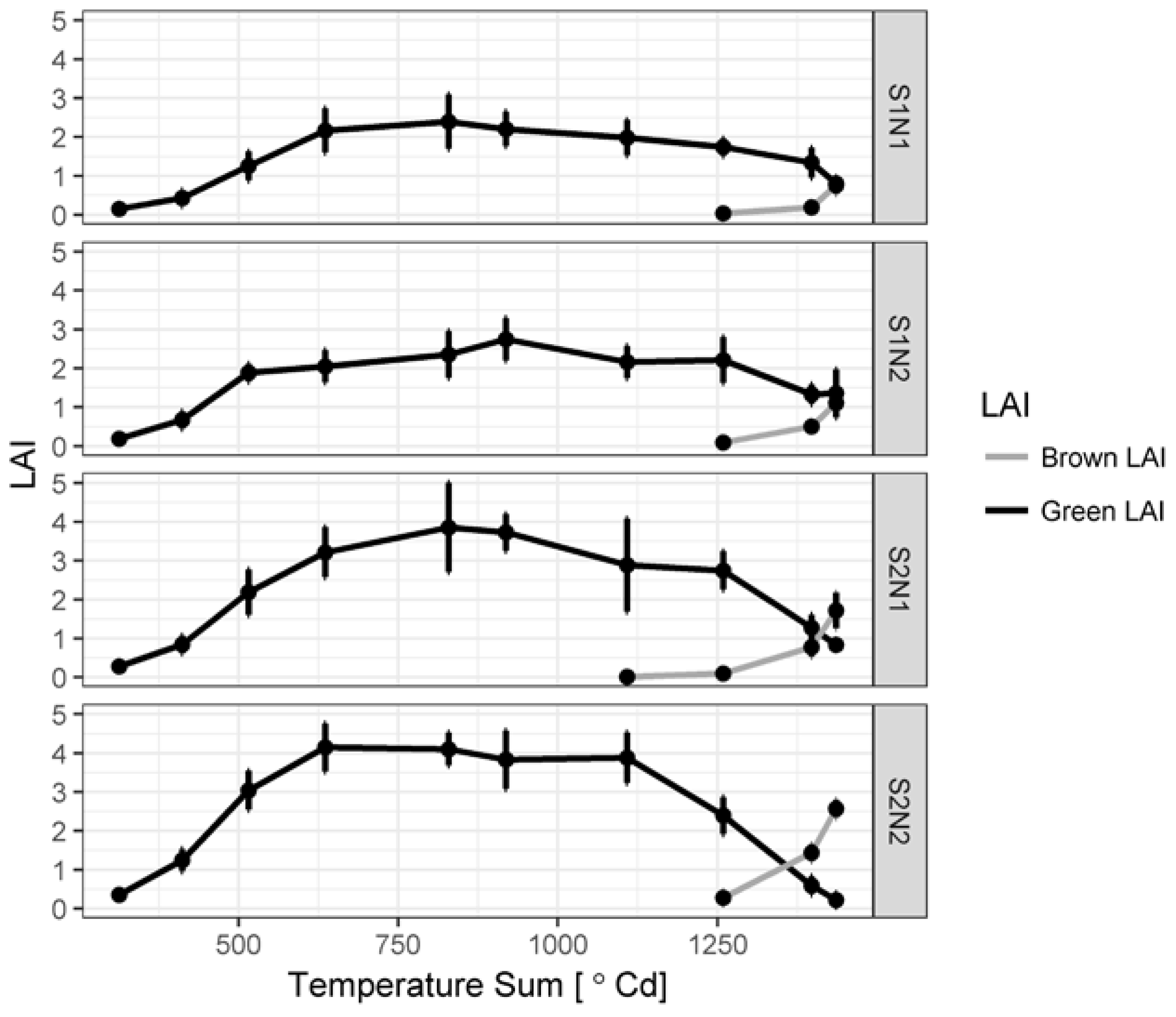
3.1. Green LAI, Brown LAI and Fractional Cover Development

The growing season 2016 passed without any major disruptive events. We took the first LAI and biomass samples in mid-June and the last samples in mid-October. The mean gLAI ranged from 0.15 to 0.35 on the first measurement day (15 June, 312 °Cd), over 2.2 to 3.83 (15 August, 918 °Cd) in mid-season to 0.75 and 2.57 on the last measurement day (16 October, 1436 °Cd). Figure 3 shows the average gLAI development per treatment. On average, gLAI values >4 were rarely measured, the absolute peak value was 5.53. Lindquist et al. [7] reported peak gLAI values between 4.8 to 7.8 in different years, Liu et al. [36] values up to 7.53 and Timlin et al. [38] average values between 2.2 and 4.28, with peak values between 3 and 5.62.

Mean brown LAI ranged between 0.75 and 2.57 on the last measurement day. Although not in focus of this study, we point out that senescence occurred earlier and faster in the high than in the low plant densities (Figure 3). Low plant densities showed more green than brown leaf area at the last measurement date, contrary to the high plant densities.

fCover ranged from 15% to 36% at the beginning of the measurement period. It increased quickly, and reached its maximum in all treatments around 828 °Cd (Figure 4), with an average of 88% to 96% of the measurement plots covered with plant tissue. fCover dropped to an average between 70% and 76% at the end of the growing season.

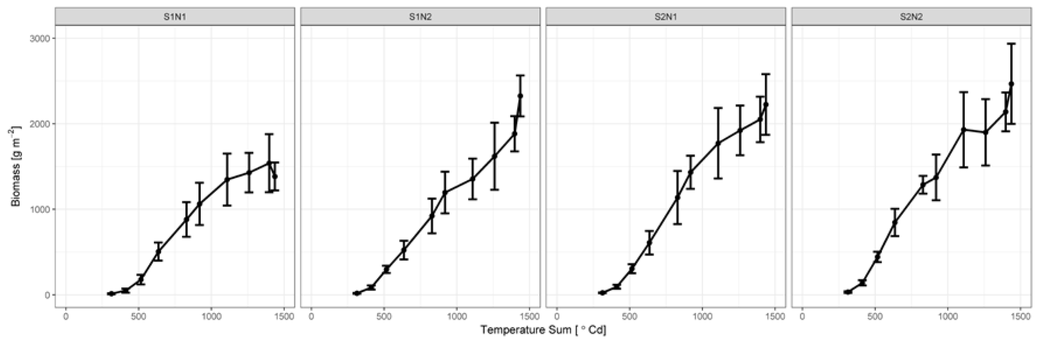
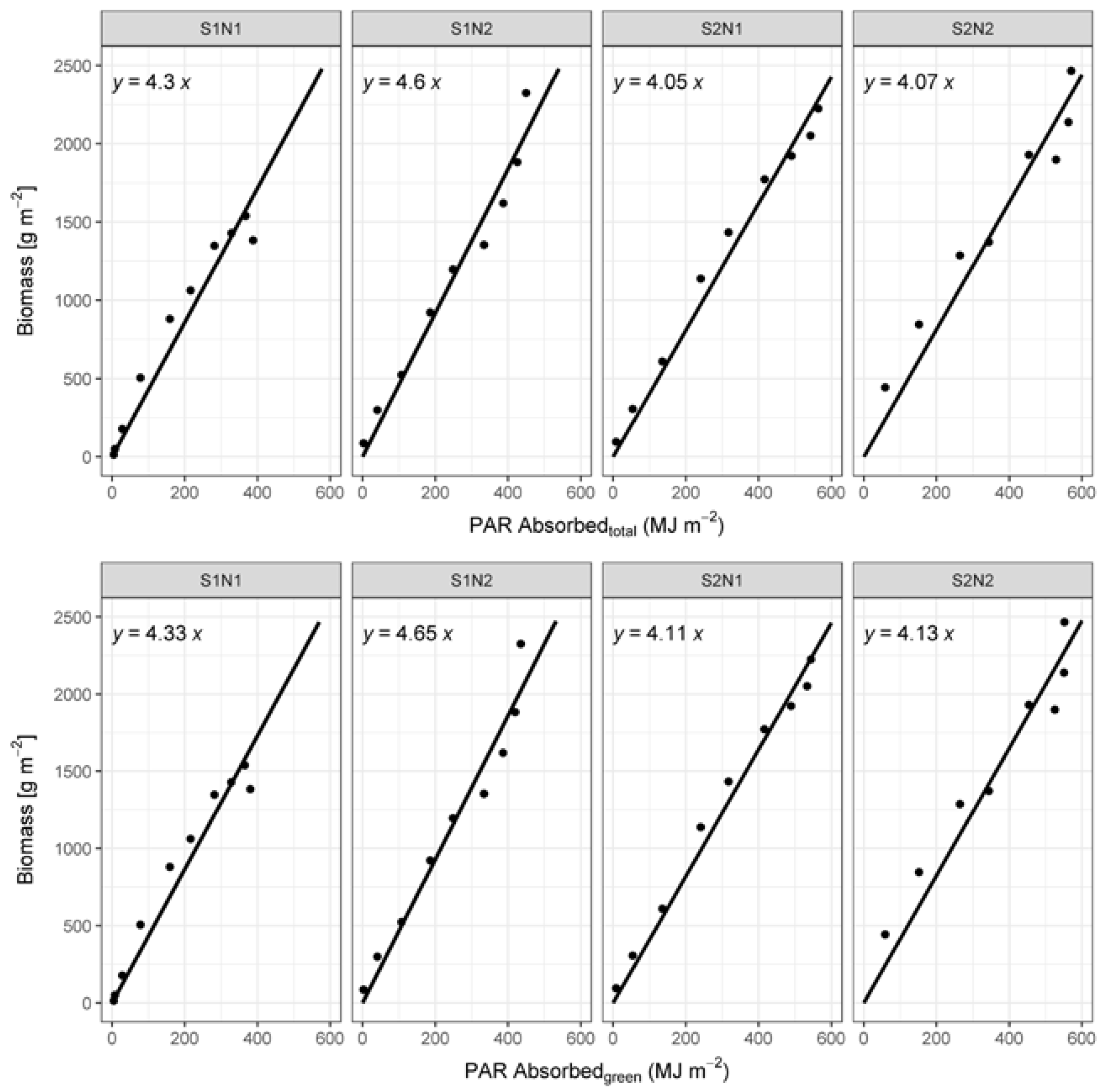
3.2. Biomass Development

The development of average biomass per treatment vs. growing degree days is shown in Figure 5. The accumulation followed a typical sigmoidal growth curve, including a decreasing accumulation rate towards the end of the growing season. Measured average values ranged between 14 g m⁻² and 32 g m⁻² on the first measurement date and between 1063 g m⁻² and 1433 g m⁻² in mid-season. The average biomass measured at the last sampling date (16 October) comprised 1384 g m⁻² in the S1N1 treatment, 2325 g m⁻² in the S1N2 treatment, 2225 g m⁻² in the S2N1 treatment and 2466 g m⁻² in the S2N2 treatment. In comparison, Lindquist et al. [7] reported total biomass values at physiological maturity between 2257 and 2916 g m⁻², Dong et al. [14] up to 2500 g m⁻².

Given the broad range of measured gLAI and biomass values measured across treatments and over time, the desired variability induced by the field experiment was obtained.

3.3. Radiation Use Efficiency Development

Figure 6 shows the sum of incoming PAR vs. fAPAR_total (left) and vs. fAPAR_green (right). The course of the curves in both plots was identical until beyond 1000 MJ m⁻² accumulated PAR. Differences were only visible towards the end of the growing season, where fAPAR_total decreased comparatively less due to the stronger influence of reflectance of the senesced leaves. fAPAR of the S2N2 treatment was the highest during most of the growing season and dropped to the lowest towards the end of the growing season. RUE_total values for different treatments were 4.3 (S1N1), 4.6 (S1N2), 4.05 (S2N1) and 4.07 (S2N2). Differences to RUE_green values were marginal, with 4.33 (S1N1), 4.65 (S1N2), 4.11 (S2N1) and 4.13 (S2N2) reported for the latter (Figure 7).

4. Discussion

In this study, we determined RUE of maize based on UAV low-cost camera imagery. We are presenting one-year data on the relationship between spectral reflectance of maize canopies, their PAR absorbed and biomass production at the same time intervals. The focal point laid on the capability to derive RUE of maize based on UAV-derived reflectance data rather than on the investigation of N and PD effects, which might vary between years. fPAR_out, biomass and LAI were measured biweekly in four different treatments, which resulted in an extraordinary comprehensive dataset, thus making yearly replications of measurement series unnecessary.

4.1. Camera Sensitivity

In this study, we assumed that the sensitivity of the red, green and blue bands of the cameras corresponded to the spectral region of PAR. The spectral sensitivity of the bands and wavelength transmittance of filters of most COTS cameras are unknown, unless exposed to monochromatic light [39]. We did not examine the response of our cameras employed. Berra et al. [39] investigated the spectral sensitivity of several unmodified and one filter-modified camera, and found that all of the unmodified cameras showed similar ranges within the visible spectrum, with almost all of the RGB channels covering the range of 400–700 nm, but with varying degrees of sensitivity and substantial band overlap [39]. The filter-modified camera exhibited well-characterized sensitivities in the visible range that were narrower and of more equal intensities than those of the unmodified cameras. We are convinced that, in our case, the influences of varying sensitivities were minimized by the band wise conversion to reflectance values. Admittedly, sensitivity curves generally follow a bell shape [39] contrary to PAR quantum sensors, which closely follows the ideal quantum response [40]. Given this and the overlapping band sensitivities, we are uncertain to make a statement about whether our approach tended to under- or overestimate true PAR reflectance. We encourage future researchers to look into this subject matter.

4.2. Green and Brown LAI Development and Measurement Techniques

For this study, green and brown LAI was measured to calculate RUE_green (see Equations (4) and (5)). Contrary to studies that rely on indirect LAI measurement methods via the transmission of radiation in the canopy, we used the direct method of harvesting the maize plants and measuring the area of all leaves within the delimited area. Compared to destructive sampling, indirect methods often underestimate LAI values in maize [41,42]. In this study, plants were harvested per area, not per count. Sampling was conducted at uncommonly very high temporal resolution (~every two weeks). Given the detailed knowledge about plant population and the precision of the measurement method, we have strong confidence in the accuracy of our measured green and brown LAI values.

However, discrepancy remains between the destructively measured area of green leaves and the functional parts of the canopy which influence the spectral signal and are sensed by the cameras, comprising not only leaves, but other parts of the crop, such as stem and husks (commonly referred to as Green Area Index) [43,44]. We are not aware of any literature that discusses a potential influence of green plant organs, apart from leaves, on reflectance and gLAI estimates by RS, especially in taller crops where organ area is hard to measure. Given the large area of leaves of maize plants, we hypothesize that the influence of other organs to the overall signal is negligible.

4.3. fAPAR Calculation Assumptions

Light attenuation in maize is influenced by canopy architecture, defined in terms of the size, shape and orientation of the aboveground components of the plant [37]. Canopy architecture is influenced by various factors such as management via plant density [38] and row spacing [45], as well as cultivar-specific properties (plant height, leaf number, leaf angle distribution). Modern maize hybrids usually have erect leaves above the ear and flat leaves below the ear [46], with erectophile hybrids usually associated with k-values < 0.5 [47]. Huang et al. [46] recently found k-values between 0.56–0.74. This shows that estimation of canopy transmittance via the Beer’s law remains a great source of uncertainty.

Contrary to other studies estimating RUE in maize, we did not cultivate the maize crops under irrigated conditions. We assume that water stress did not occur at any time, given the amount of precipitation that fell over the course of the growing season. We furthermore calculated soil moisture retention from data of a physical soil properties analysis [25] and concluded that soil-moisture tension did not exceed pF values of 3 in 30 cm soil depth until flowering, and at no point in time in 60 cm and 90 cm soil depth (soil moisture measured with EC-5 sensors (Decagon Devices Inc., Pullman, WA, USA) installed in-between the two mid-rows of the unsampled plots, data not shown). Additionally, we did not observe leaf rolling, which is one of the main plant reactions to water stress. Given this, heat stress is also assumed to be minimal, since the critical canopy temperature is generally reduced by the cooling effect of water transpiration [48]. Our approach furthermore assumed that PAR_soil absorbed by the canopy comprises radiation transmitted through the canopy only; we neglected directional or diffuse reflection from the surrounding area of the plants. The influence was possibly larger during early growing stages before canopy closure. Especially illuminated soil in-between the rows, which was not covered by leaf tissue yet, could have contributed to PAR absorption to a larger extent. Additionally, the contribution of varying soil moisture to the PAR_soil remains unknown. Wet soils commonly reflect less PAR than dry soils [49]. A number of studies neglected PAR_soil altogether, assuming to have only little influence on APAR (e.g., [7,50]). Gallo and Daughtry [51] found that intercepted PAR (i.e., 1-PAR_trans) overestimated APAR in a maize canopy throughout most of the growing season by less than 4%, which emphasizes the little influence of PAR_soil on total APAR.

4.4. RUE Values

The RUE values derived in this study were higher than those published in recent articles. Lindquist et al. [7] found an RUE of 3.8 g MJ⁻¹ APAR for aboveground biomass accumulation, PAR_soil was not measured. We consider the values presented here plausible, given the trends in biomass increase induced by improved plant breeding. Biomass increase in modern maize hybrids is mostly attributable to higher plant density tolerance [52], which results from increased light intensity in the mid and lower canopy layers. Maize adapts to increased density by increasing leaf spacing below the ear and the leaf orientation above the ear, and by reducing leaf width and leaf angle [53]. Lower RUE in high plant densities could be a result of decreased absorption efficiency due to more self-shading.

In agreement with Lindquist et al. [7], we also cannot support the common perception that RUE declines during grain fill. Both absorption and biomass increase occurred until the last sampling date.

Unfortunately, no statistical analysis was possible to determine differences or similarities between RUE_green and RUE_total, and the impact of different treatments. RUE_green and RUE_total values of the same treatments did not differ considerably. Figure 6 furthermore suggests that a difference between fAPAR_total and fAPAR_green only occurred towards the end of the growing season, around the full ripening stage. The influence of the stay green trait possibly caused this; the longer maintenance of greenness resulted in a weak influence of senesced material to plant reflectance. Although both approaches produce similar results, we nevertheless recommend relying on the RUE_green concepts, since the onset of senescence is both cultivar- and weather driven.

Since root mass is difficult to measure, it is commonly not included in RUE estimations. The inclusion would inevitably result in higher values. Root mass of maize around anthesis may comprise 15% to 40% of the total crop mass. N fertilization might decrease root mass or show no impact at all [54].

As mentioned above, we computed RUE via cumulative APAR. However, Mitchell et al. [55] pointed out that this method gives false confidence in the true actual value of RUE and so obscures all variation in RUE with time. In fact, the temporal behaviour of RUE is characterized by short term facultative (day-to-day) and long term constitutive (seasonal) variations [6]. RUE_green can vary more than three-fold over the season with no clear pattern, and additionally show day-to-day variability, depending on the physiological status of the vegetation. The daily variability of PAR also causes RUE_green day-to-day oscillation, with a decrease due to excessive PAR_inc, which cannot be efficiently used by the maize plant. The long-term variation is affected by the physiological status and phenology, furthermore by the temporal changes of green and brown plant tissue [6].

5. Conclusions

This study showed that UAV-based reflectance data derived from low-cost camera imagery could be used to support the derivation of RUE values in small-scale experimental plots (provided that the data is well-preprocessed). The great advantage of this approach is that fractional cover and fPAR_out as necessary inputs for the calculation of RUE can be sensed over larger areas, and not just point-based. Possibly, the above-mentioned parameters could be mapped at small spatial scales (e.g., m²) in fields, thereby revealing heterogeneous patterns that would otherwise remain undetected. A cultivar-dependent RUE derivation is possible; this gives crop modelers the chance to improve radiation-driven crop growth models. gLAI can also be mapped with the help of UAVs and multispectral or hyperspectral cameras; the mapping of brown LAI is encouraged to be focus of research in future activities. First studies on the estimation of standing biomass in cereals via UAV-based RS were recently published [17,18,56]. Taking this under consideration, the need for labor-intensive, costly field measurements could be reduced to a minimum.

References

1. Stöckle, C.O.; Kemanian, A.R. Crop Radiation Capture and Use Efficiency: A Framework for Crop Growth Analysis. In Crop Physiology; Academic Press: San Diego, CA, USA, 2009; Chapter 7; pp. 145–170. ISBN 978-0-12-374431-9. [Google Scholar]
2. Monteith, J.L. The management of inputs for yet greater agricultural yield and efficiency-Climate and the efficiency of crop production in Britain. Philos. Trans. R. Soc. Lond. B 1977, 281, 277–294. [Google Scholar] [CrossRef]
3. Morel, J.; Bégué, A.; Todoroff, P.; Martiné, J.-F.; Lebourgeois, V.; Petit, M. Coupling a sugarcane crop model with the remotely sensed time series of fIPAR to optimise the yield estimation. Eur. J. Agron. 2014, 61, 60–68. [Google Scholar] [CrossRef]
4. Sinclair, T.R.; Muchow, R.C. Radiation Use Efficiency. Adv. Agron. 1999, 65, 215–265. [Google Scholar] [CrossRef]
5. Gitelson, A.A.; Gamon, J.A. The need for a common basis for defining light-use efficiency: Implications for productivity estimation. Remote Sens. Environ. 2015, 156, 196–201. [Google Scholar] [CrossRef]
6. Gitelson, A.A.; Peng, Y.; Arkebauer, T.J.; Suyker, A.E. Productivity, absorbed photosynthetically active radiation, and light use efficiency in crops: Implications for remote sensing of crop primary production. J. Plant Physiol. 2015, 177, 100–109. [Google Scholar] [CrossRef] [PubMed]
7. Lindquist, J.L.; Arkebauer, T.J.; Walters, D.T.; Cassman, K.G.; Dobermann, A. Maize radiation use efficiency under optimal growth conditions. Agron. J. 2005, 97, 72–78. [Google Scholar] [CrossRef]
8. Viña, A.; Gitelson, A.A. New developments in the remote estimation of the fraction of absorbed photosynthetically active radiation in crops. Geophys. Res. Lett. 2005, 32. [Google Scholar] [CrossRef]
9. Luche, H.D.S.; Silva, J.A.G.D.; Maia, L.C.D.; Oliveira, A.C.D. Stay-green: A potentiality in plant breeding. Ciênc. Rural 2015, 45, 1755–1760. [Google Scholar] [CrossRef]
10. Antonietta, M.; Acciaresi, H.A.; Guiamet, J.J. Responses to N Deficiency in Stay Green and Non-Stay Green Argentinean Hybrids of Maize. J. Agron. Crop Sci. 2016, 202, 231–242. [Google Scholar] [CrossRef]
11. Swanckaert, J.; Pannecoucque, J.; Waes, J.V.; Steppe, K.; Labeke, M.-C.V.; Reheul, D. Stay-green characterization in Belgian forage maize. J. Agric. Sci. 2017, 155, 766–776. [Google Scholar] [CrossRef]
12. Singer, J.W.; Meek, D.W.; Sauer, T.J.; Prueger, J.H.; Hatfield, J.L. Variability of light interception and radiation use efficiency in maize and soybean. Field Crops Res. 2011, 121, 147–152. [Google Scholar] [CrossRef]
13. Claverie, M.; Demarez, V.; Duchemin, B.; Hagolle, O.; Ducrot, D.; Marais-Sicre, C.; Dejoux, J.-F.; Huc, M.; Keravec, P.; Béziat, P.; et al. Maize and sunflower biomass estimation in southwest France using high spatial and temporal resolution remote sensing data. Remote Sens. Environ. 2012, 124, 844–857. [Google Scholar] [CrossRef] [Green Version]
14. Dong, T.; Liu, J.; Qian, B.; Jing, Q.; Croft, H.; Chen, J.; Wang, J.; Huffman, T.; Shang, J.; Chen, P. Deriving Maximum Light Use Efficiency From Crop Growth Model and Satellite Data to Improve Crop Biomass Estimation. IEEE J. Sel. Top. Appl. Earth Obs. Remote Sens. 2017, 10, 104–117. [Google Scholar] [CrossRef]
15. Gitelson, A.A.; Peng, Y.; Arkebauer, T.J.; Schepers, J. Relationships between gross primary production, green LAI, and canopy chlorophyll content in maize: Implications for remote sensing of primary production. Remote Sens. Environ. 2014, 144, 65–72. [Google Scholar] [CrossRef]
16. Jones, H.G.; Vaughan, R.A. Remote Sensing of Vegetation: Principles, Techniques, and Applications; Oxford University Press: Oxford, UK, 2010; ISBN 978-0-19-920779-4. [Google Scholar]
17. Bendig, J.; Bolten, A.; Bennertz, S.; Broscheit, J.; Eichfuss, S.; Bareth, G. Estimating Biomass of Barley Using Crop Surface Models (CSMs) Derived from UAV-Based RGB Imaging. Remote Sens. 2014, 6, 10395–10412. [Google Scholar] [CrossRef]
18. Yue, J.; Yang, G.; Li, C.; Li, Z.; Wang, Y.; Feng, H.; Xu, B. Estimation of Winter Wheat Above-Ground Biomass Using Unmanned Aerial Vehicle-Based Snapshot Hyperspectral Sensor and Crop Height Improved Models. Remote Sens. 2017, 9, 708. [Google Scholar] [CrossRef]
19. Córcoles, J.I.; Ortega, J.F.; Hernández, D.; Moreno, M.A. Estimation of leaf area index in onion (Allium cepa L.) using an unmanned aerial vehicle. Biosyst. Eng. 2013, 115, 31–42. [Google Scholar] [CrossRef]
20. Hunt, E.R.; Hively, W.D.; Fujikawa, S.J.; Linden, D.S.; Daughtry, C.S.T.; McCarty, G.W. Acquisition of NIR-Green-Blue Digital Photographs from Unmanned Aircraft for Crop Monitoring. Remote Sens. 2010, 2, 290–305. [Google Scholar] [CrossRef]
21. Burkart, A.; Hecht, V.L.; Kraska, T.; Rascher, U. Phenological analysis of unmanned aerial vehicle based time series of barley imagery with high temporal resolution. Precis. Agric. 2017, 1–13. [Google Scholar] [CrossRef]
22. Haghighattalab, A.; Crain, J.; Mondal, S.; Rutkoski, J.; Singh, R.P.; Poland, J. Application of Geographically Weighted Regression to Improve Grain Yield Prediction from Unmanned Aerial System Imagery. Crop Sci. 2017, 57, 2478–2489. [Google Scholar] [CrossRef]
23. Maresma, Á.; Ariza, M.; Martínez, E.; Lloveras, J.; Martínez-Casasnovas, J.A. Analysis of Vegetation Indices to Determine Nitrogen Application and Yield Prediction in Maize (Zea mays L.) from a Standard UAV Service. Remote Sens. 2016, 8, 973. [Google Scholar] [CrossRef]
24. Zhou, X.; Zheng, H.B.; Xu, X.Q.; He, J.Y.; Ge, X.K.; Yao, X.; Cheng, T.; Zhu, Y.; Cao, W.X.; Tian, Y.C. Predicting grain yield in rice using multi-temporal vegetation indices from UAV-based multispectral and digital imagery. ISPRS J. Photogramm. Remote Sens. 2017, 130, 246–255. [Google Scholar] [CrossRef]
25. Gaiser, T.; Perkons, U.; Küpper, P.M.; Puschmann, D.U.; Peth, S.; Kautz, T.; Pfeifer, J.; Ewert, F.; Horn, R.; Köpke, U. Evidence of improved water uptake from subsoil by spring wheat following lucerne in a temperate humid climate. Field Crops Res. 2012, 126, 56–62. [Google Scholar] [CrossRef]
26. Kautz, T.; Stumm, C.; Kösters, R.; Köpke, U. Effects of perennial fodder crops on soil structure in agricultural headlands. J. Plant Nutr. Soil Sci. 2010, 173, 490–501. [Google Scholar] [CrossRef]
27. Birch, C.J.; Vos, J.; van der Putten, P.E.L. Plant development and leaf area production in contrasting cultivars of maize grown in a cool temperate environment in the field. Eur. J. Agron. 2003, 19, 173–188. [Google Scholar] [CrossRef] [Green Version]
28. Jonckheere, I.; Fleck, S.; Nackaerts, K.; Muys, B.; Coppin, P.; Weiss, M.; Baret, F. Review of methods for in situ leaf area index determination: Part I. Theories, sensors and hemispherical photography. Agric. For. Meteorol. 2004, 121, 19–35. [Google Scholar] [CrossRef]
29. Kelcey, J.; Lucieer, A. Sensor Correction of a 6-Band Multispectral Imaging Sensor for UAV Remote Sensing. Remote Sens. 2012, 4, 1462–1493. [Google Scholar] [CrossRef]
30. Smith, G.M.; Milton, E.J. The use of the empirical line method to calibrate remotely sensed data to reflectance. Int. J. Remote Sens. 1999, 20, 2653–2662. [Google Scholar] [CrossRef]
31. R Core Team. R: A Language and Environment for Statistical Computing; R Foundation for Statistical Computing: Vienna, Austria, 2017. [Google Scholar]
32. Leutner, B.; Horning, N. RStoolbox: Tools for Remote Sensing Data Analysis. 2017. CRAN–Package RStoolbox. Available online: https://cran.r-project.org/web/packages/RStoolbox/index.html (accessed on 5 February 2018).
33. Ghamisi, P.; Plaza, J.; Chen, Y.; Li, J.; Plaza, A.J. Advanced Spectral Classifiers for Hyperspectral Images: A review. IEEE Geosci. Remote Sens. Mag. 2017, 5, 8–32. [Google Scholar] [CrossRef]
34. Rodriguez-Galiano, V.F.; Ghimire, B.; Rogan, J.; Chica-Olmo, M.; Rigol-Sanchez, J.P. An assessment of the effectiveness of a random forest classifier for land-cover classification. ISPRS J. Photogramm. Remote Sens. 2012, 67, 93–104. [Google Scholar] [CrossRef]
35. Hijmans, R.J. Raster: Geographic Data Analysis and Modeling. 2016. CRAN–Package Raster. Available online: https://cran.r-project.org/web/packages/raster/index.html (accessed on 5 February 2018).
36. Liu, G.; Hou, P.; Xie, R.; Ming, B.; Wang, K.; Xu, W.; Liu, W.; Yang, Y.; Li, S. Canopy characteristics of high-yield maize with yield potential of 22.5 Mgha−1. Field Crops Res. 2017, 213, 221–230. [Google Scholar] [CrossRef]
37. Maddonni, G.A.; Otegui, M.E.; Cirilo, A.G. Plant population density, row spacing and hybrid effects on maize canopy architecture and light attenuation. Field Crops Res. 2001, 71, 183–193. [Google Scholar] [CrossRef]
38. Timlin, D.J.; Fleisher, D.H.; Kemanian, A.R.; Reddy, V.R. Plant Density and Leaf Area Index Effects on the Distribution of Light Transmittance to the Soil Surface in Maize. Agron. J. 2014, 106, 1828. [Google Scholar] [CrossRef]
39. Berra, E.; Gibson-Poole, S.; MacArthur, A.; Gaulton, R.; Hamilton, A. Estimation of the spectral sensitivity functions of un-modified and modified commercial off-the-shelf digital cameras to enable their use as a multispectral imaging system for UAVs. ISPRS-Int. Arch. Photogramm. Remote Sens. Spat. Inf. Sci. 2015, XL-1/W4, 207–214. [Google Scholar] [CrossRef]
40. Ross, J.; Sulev, M. Sources of errors in measurements of PAR. Agric. For. Meteorol. 2000, 100, 103–125. [Google Scholar] [CrossRef]
41. Bréda, N.J.J. Ground-based measurements of leaf area index: A review of methods, instruments and current controversies. J. Exp. Bot. 2003, 54, 2403–2417. [Google Scholar] [CrossRef] [PubMed]
42. Wilhelm, W.W.; Ruwe, K.; Schlemmer, M.R. Comparison of three leaf area index meters in a corn canopy. Crop Sci. 2000, 40, 1179–1183. [Google Scholar] [CrossRef]
43. Baret, F.; de Solan, B.; Lopez-Lozano, R.; Ma, K.; Weiss, M. GAI estimates of row crops from downward looking digital photos taken perpendicular to rows at 57.5° zenith angle: Theoretical considerations based on 3D architecture models and application to wheat crops. Agric. For. Meteorol. 2010, 150, 1393–1401. [Google Scholar] [CrossRef]
44. Verger, A.; Vigneau, N.; Chéron, C.; Gilliot, J.-M.; Comar, A.; Baret, F. Green area index from an unmanned aerial system over wheat and rapeseed crops. Remote Sens. Environ. 2014, 152, 654–664. [Google Scholar] [CrossRef]
45. Andrade, F.H.; Calviño, P.; Cirilo, A.; Barbieri, P. Yield Responses to Narrow Rows Depend on Increased Radiation Interception. Agron. J. 2002, 94, 975. [Google Scholar] [CrossRef]
46. Huang, S.; Gao, Y.; Li, Y.; Xu, L.; Tao, H.; Wang, P. Influence of plant architecture on maize physiology and yield in the Heilonggang River valley. Crop J. 2017, 5, 52–62. [Google Scholar] [CrossRef]
47. Ma, D.L.; Xie, R.Z.; Niu, X.K.; Li, S.K.; Long, H.L.; Liu, Y.E. Changes in the morphological traits of maize genotypes in China between the 1950s and 2000s. Eur. J. Agron. 2014, 58, 1–10. [Google Scholar] [CrossRef]
48. Gabaldón-Leal, C.; Webber, H.; Otegui, M.E.; Slafer, G.A.; Ordóñez, R.A.; Gaiser, T.; Lorite, I.J.; Ruiz-Ramos, M.; Ewert, F. Modelling the impact of heat stress on maize yield formation. Field Crops Res. 2016, 198, 226–237. [Google Scholar] [CrossRef]
49. Lobell, D.B.; Asner, G.P. Moisture effects on soil reflectance. Soil Sci. Soc. Am. J. 2002, 66, 722–727. [Google Scholar] [CrossRef]
50. Tollenaar, M.; Aguilera, A. Radiation use efficiency of an old and a new maize hybrid. Agron. J. 1992, 84, 536–541. [Google Scholar] [CrossRef]
51. Gallo, K.P.; Daughtry, C.S.T. Techniques for Measuring Intercepted and Absorbed Photosynthetically Active Radiation in Corn Canopies. Agron. J. 1986, 78, 752–756. [Google Scholar] [CrossRef]
52. Antonietta, M.; Fanello, D.D.; Acciaresi, H.A.; Guiamet, J.J. Senescence and yield responses to plant density in stay green and earlier-senescing maize hybrids from Argentina. Field Crops Res. 2014, 155, 111–119. [Google Scholar] [CrossRef]
53. Gou, L.; Xue, J.; Qi, B.; Ma, B.; Zhang, W. Morphological Variation of Maize Cultivars in Response to Elevated Plant Densities. Agron. J. 2017, 109, 1443. [Google Scholar] [CrossRef]
54. Anderson, E.L. Tillage and N fertilization effects on maize root growth and root:shoot ratio. Plant Soil 1988, 108, 245–251. [Google Scholar] [CrossRef]
55. Mitchell, P.L.; Sheehy, J.E.; Woodward, F.I. Potential Yields and the Efficiency of Radiation Use in Rice; IRRI Discussion Paper Series; International Rice Research Institute: Manila, Philippines, 1998; Volume 32. [Google Scholar]
56. Li, W.; Niu, Z.; Chen, H.; Li, D.; Wu, M.; Zhao, W. Remote estimation of canopy height and aboveground biomass of maize using high-resolution stereo images from a low-cost unmanned aerial vehicle system. Ecol. Indic. 2016, 67, 637–648. [Google Scholar] [CrossRef]
Figure 1. Example of an original image (left), the classification (center) with green representing plant tissue, brown representing illuminated soil, and black representing shaded soil. The third image (right) shows original image after removal of soil pixels. Black rectangles delineate spots where plants were later sampled destructively for LAI and biomass measurements.
Agronomy 08 00016 g001
Figure 2. Flowchart of the RUEtotal and RUEgreen estimation method.
Agronomy 08 00016 g002
Figure 3. Green and Brown LAI development over the course of the growing season 2016. Error bars show standard deviation.
Agronomy 08 00016 g003
Figure 4. Fractional cover development over the course of the growing season 2016. Error bars show standard deviation. The horizontal position was adjusted to avoid overlap.
Agronomy 08 00016 g004
Figure 5. Dry biomass development per treatment. Error bars show standard deviation.
Agronomy 08 00016 g005
Figure 6. fAPARtotal (left) and fAPARgreen (right) vs. Sum of Incoming PAR. Each line represents one treatment.
Agronomy 08 00016 g006
Figure 7. Cumulative maize aboveground biomass as a function of cumulative absorbed photosynthetically active radiation. The top row shows relationship per treatment based on APARtotal, the bottom row based on APARgreen. The slope of the estimated regression equation is the RUE. The intercept was suppressed.
Agronomy 08 00016 g007