Existing and Potential Statistical and Computational Approaches for the Analysis of 3D CT Images of Plant Roots


1
Department of Statistics, University of Nebraska-Lincoln, Lincoln, NE 68583, USA
2
School of Computing and Information Sciences, Florida International University, Miami, FL 33199, USA
3
Department of Food Science and Technology, University of Nebraska-Lincoln, Lincoln, NE 68588, USA
*
Author to whom correspondence should be addressed.
†
These authors contributed equally to this work.
Agronomy 2018, 8(5), 71; https://doi.org/10.3390/agronomy8050071
Submission received: 11 April 2018
/
Revised: 24 April 2018
/
Accepted: 9 May 2018
/
Published: 14 May 2018
(This article belongs to the Special Issue Precision Phenotyping in Plant Breeding)
Abstract
:Scanning technologies based on X-ray Computed Tomography (CT) have been widely used in many scientific fields including medicine, nanosciences and materials research. Considerable progress in recent years has been made in agronomic and plant science research thanks to X-ray CT technology. X-ray CT image-based phenotyping methods enable high-throughput and non-destructive measuring and inference of root systems, which makes downstream studies of complex mechanisms of plants during growth feasible. An impressive amount of plant CT scanning data has been collected, but how to analyze these data efficiently and accurately remains a challenge. We review statistical and computational approaches that have been or may be effective for the analysis of 3D CT images of plant roots. We describe and comment on different approaches to aspects of the analysis of plant roots based on images, namely, (1) root segmentation, i.e., the isolation of root from non-root matter; (2) root-system reconstruction; and (3) extraction of higher-level phenotypes. As many of these approaches are novel and have yet to be applied to this context, we limit ourselves to brief descriptions of the methodologies. With the rapid development and growing use of X-ray CT scanning technologies to generate large volumes of data relevant to root structure, it is timely to review existing and potential quantitative and computational approaches to the analysis of such data. Summaries of several computational tools are included in the Appendix.
1. Introduction
The use of X-ray Computed Tomography (CT) scanning of plant roots is an important part of the integration of modern technologies in biological and agricultural research. The earliest implementations of X-ray CT for plant research date back to 30 years ago [1]. Since X-ray CT scanners were originally designed for medical applications (and then for industrial applications), some adjustments to the image preprocessing and segmentation to accommodate root structures have been necessary. In medical images, tubular structures are often of higher grayscale intensity values (the range of gray color values) than the surrounding tissues—the structures have different X-ray absorption coefficients—making them easier to detect than roots that do not share this property. Plants may be grown in substrates whose intensities overlap; plant root systems have varying topologies and tissue components; and it may be nontrivial to combine 2D cross-sectional images into a single 3D image. There are other challenges related to X-ray CT imaging for leaf canopy scanning [2], root imaging in the field [3,4], and rhizosphere quantification [5,6]. These include image normalization, destructive vs. nondestructive sampling, dynamic modeling, and significant manual labor.
X-ray CT scanning of plant roots has received considerable attention in the last few years with the development of high-throughput plant phenotyping technologies. There are several reasons for this, including but not limited to (1) the development of cabinet or benchtop lab scanners with improved detector technology; (2) scanners with faster and higher resolution imaging capabilities; (3) imaging of roots in natural soils (including the soil-root interface); and (4) the ability to monitor dynamic root development through nondestructive sampling [7]. These technologies have enabled the plant sciences community, as well as collaborators from other disciplines, to take a closer look at root morphology, root system architecture (RSA), and the dynamics of root growth. It is well recognized that plant root anatomy and architecture depend on genetics [8] as well as nutrients in the soil such as phosphorus, potassium, and nitrogen [9,10]. It has also been established that the soil substrate influences root anatomy; see, for example, Ahmed et al. [11] and Rich and Watt [12]. Important influences on root development may come from abiotic stressors such as drought, salinity, and extreme temperature [13,14] not to mention biotic stressors such as pathogens [15,16,17,18]. One important biotic stressor—or helper—of particular recent interest is the rhizosphere and root-rhizosphere interactions [19,20,21]. The study of such interactions is enabled by non-destructive phenotyping technologies that can examine the phenotypic impacts of such interactions in soil during the stages of growth [22]. Such impacts are captured by phenotypic traits, i.e., qualitative and quantitative measures that describe the appearance of plants and their roots [23,24].
Several research groups have invested heavily in non-destructive imaging technologies for roots, including X-ray CT imaging [25]. A significant challenge with X-ray CT imaging (as with Magnetic Resonance Imaging (MRI) [26]) is the processing and analysis of the resulting images [7]. These images tend to be large, requiring substantial computational resources, and the discrimination of roots from the surrounding substrates can be a considerable challenge. This is unlike most medical applications of X-ray CT imaging where different biological structures (such as bones and high-water content organs such as the liver, brain, etc.) can be easily discriminated based on the resulting grayscale intensity values [27]. However, given the ability of X-ray CT and similar imaging technologies to examine plant roots and tuberous crops in situ and the global challenge of increasing food production given limited resources [28], the scientific community is highly motivated to overcome these challenges.
In this paper we will provide a brief overview of X-ray CT data and discuss several recent statistical approaches to image analysis and feature segmentation that may be relevant to X-ray CT root phenotyping. We also provide a brief overview in Section 6 of the relevant computational software for root system tracking and 3D CT image processing such as ImageJ/Root1, RooTrak, and VG Studio Max.
2. X-ray CT Imaging
In traditional medical and clinical applications, X-ray computed tomography (CT) uses X-rays to generate tomographic images (i.e., imaging by sections or sectioning via penetrating waves) of internal objects (organs, bones, etc.). Owing to the success of CT scanning in medical domains, the application of CT scanning in plant phenotyping has grown [7]. The attenuation of rays-caused by, for example, biological matter or water-together with rotation and axial movements of a sensor over objects produces 3D images [29]. A high-throughput X-ray CT phenotyping system can be much more efficient than manual assessment of roots based primarily on decreases in the amount of manual labor involved. This efficiency must be balanced with the higher costs of CT phenotyping, which may be prohibitive for large studies.
A data set generated from a CT technology is typically comprised of transformations of the raw CT numbers, which are saved in standard medical image format with 8 bits, 16 bits or 32 bits for each voxel [30]. (Recall that 1 byte is equal to 8 bits). The CT number (CTN), expressed in terms of Hounsfield units, can be used to measure the attenuation of the material relative to the water. The formula is
where is the attenuation coefficient (Beer-Lambert law) for the X-ray beam [29,31,32]. By definition, the vacuum has a value of and water has a value of 0. Materials through which an X-ray beam decays faster than water have positive CT numbers, whereas materials through which the X-ray decays slower than water have negative CT numbers. X-ray scanning technologies can produce a CT number for each voxel—the constituent element of a volumetric three-dimensional space, and the analog of a pixel in a 2D image—in the space which is later transformed to a cube, i.e., three-dimensional array of numerical values or 3D CT scanning/image data, for researchers. Voxel depth is the number of bits used to encode the information of each voxel. With a voxel depth of 2 bytes per pixel, it is possible to codify and store integer numbers between 0 and 65,535; alternatively, it is possible to represent integer numbers between −32,768 and +32,767 using 15 bits to represent the numbers and 1 bit to represent the sign. Although less common, image data may also be real numbers. The Institute of Electrical and Electronics Engineers created a standard (IEEE-754) which defines two basic formats for the encoding in binary of floating-point numbers: the single precision 32-bit and the double precision 64-bit [30].
CT datasets are filled with noise created by the capturing instrument, X-rays, beam detectors, and onboard electronics all contribute noise to the resulting images. Tjong et. al. [33] found that datasets with high resolution voxels (41 m) performed better than those with lower resolution voxels (123 m); this was also found by Christiansen [34]. Downstream analyses (and accuracy) were affected by the choice of voxel size, and software tools needed to be calibrated and tuned for each size to properly segment and extract the features of interest. While low resolution datasets (large voxel size) tend to have smaller data footprints, their accuracy is comparatively lower than those with high resolution (small voxel size). Acquisition parameters could have an impact on downstream analysis pipelines if the analyses to be performed require a lot of computational resources (RAM, disk, CPU). For example, training an artificial neural network (ANN) can be computationally expensive, and if the training datasets are large, then the training step could be expensive (both computationally and economically).
Based on 3D X-ray CT data, one crucial issue in root analysis is root segmentation, i.e., the determination of whether a particular voxel in the space is classified as “root” or “non-root”. Unlike roots in transparent liquid solutions, which can be clearly identified from visible images [35], roots in organic soils are difficult to segment from other materials (water, air, etc.) because the root and non-root voxels have overlapping CTN values [36]. Hence, thresholding based solely on intensity values within the CT image cube will and has failed. Researchers have developed many methods in their attempts to solve this problem.
The second crucial issue is regarding the use of an initial segmentation method before further post-processing of images. Image segmentation is the process of partitioning a digital image into multiple segments, i.e., set of pixels. In root segmentation a minimum of two class labels (k, with ) may be used to distinguish between non-plant (non-root) voxels and plant (root) voxels. There are several segmentation approaches initially from the field of computer vision and the choice of method depends on specific data sets and typically innovative multiple-step and combined approaches used to improve accuracy. Some commonly-used segmentation approaches in phenotyping are (1) thresholding methods; (2) region growing approaches; (3) split-and-merge algorithm; (4) watershed segmentation; (5) statistical Markov random field methods which make use of neighboring information; and
(6) clustering approaches such as k-means clustering and nearest neighbors. Interested readers may refer to these resources for the details of each method [37,38,39].
The third crucial issue is the post-processing of image segmentation results for improving the performance of root-system reconstruction methods. Post-processing is often required after various segmentation methods have been applied—methods such as watershed segmentation, deep-learning segmentation, and thresholding-based segmentation—because researchers have found that image segmentation often leads to undesired properties and artifacts such as isolated small components or small holes and disconnections in identified objects [38]. Post-processing after segmentation has been a general topic for most types of images including visible (Red Green Blue (RGB)), MRI, and X-ray CT images. Simple post-processing approaches include morphological operations (erosion, closedness, etc.) and components filtering [38]. Approaches with more complicated and multiple steps have been proposed to deal with different research subjects and situations. For example, in segmenting skin lesions in dermoscopy images, the post-processing procedure after first-pass watershed segmentation was proposed as: (1) a neural network classifier to improve the first-pass watershed segmentation; (2) a novel “Edge Object Value (EOV) Threshold” method to remove large light blobs near the lesion boundary; and (3) a noise removal procedure to reduce the peninsula-shaped false-positive areas [40]. In another example of three-dimensional segmentation, post-processing was followed by deep learning segmentation using a convolutional neural network (CNN). The post-processing procedure was described as follows: (1) calculate the centroid of all voxels labeled as one class and the centroid of all voxels labeled as another class; (2) divide up the image into blobs (connected voxels with the same classification), and for each blob, check the size; (3) relabel blobs from either class with small sizes less than threshold as belonging to the other class [41].
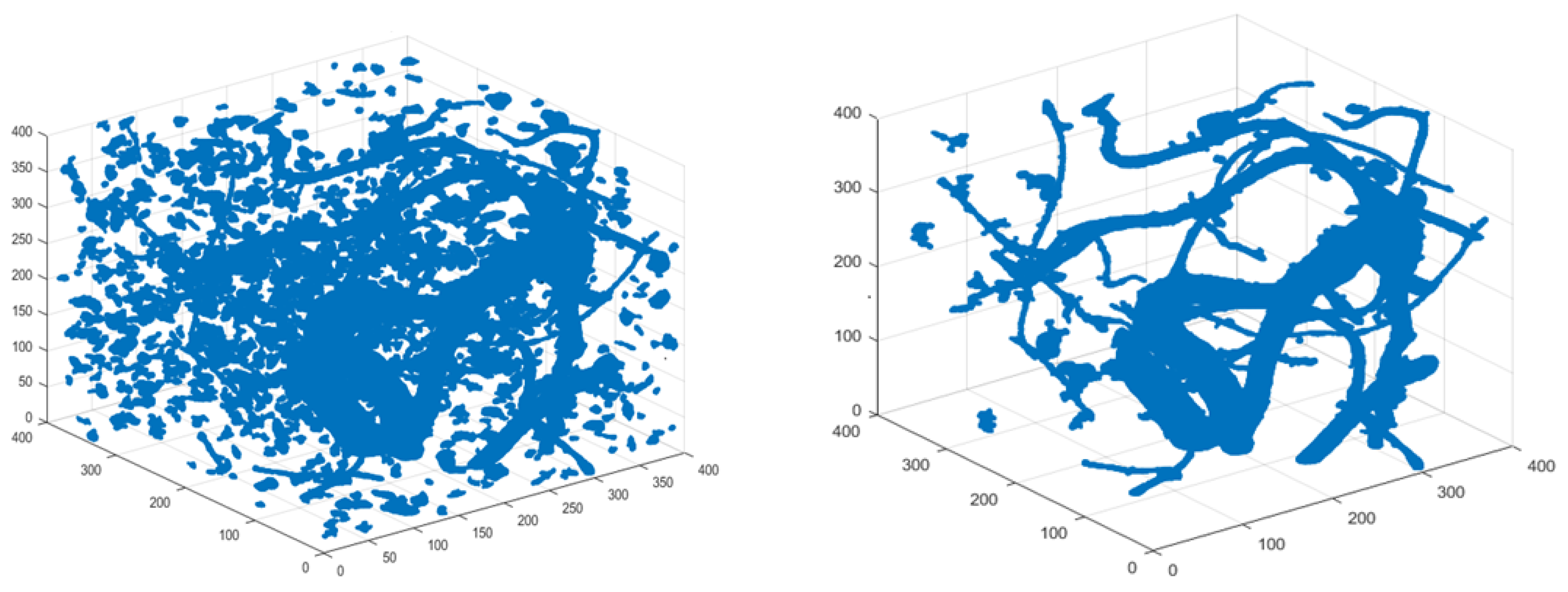
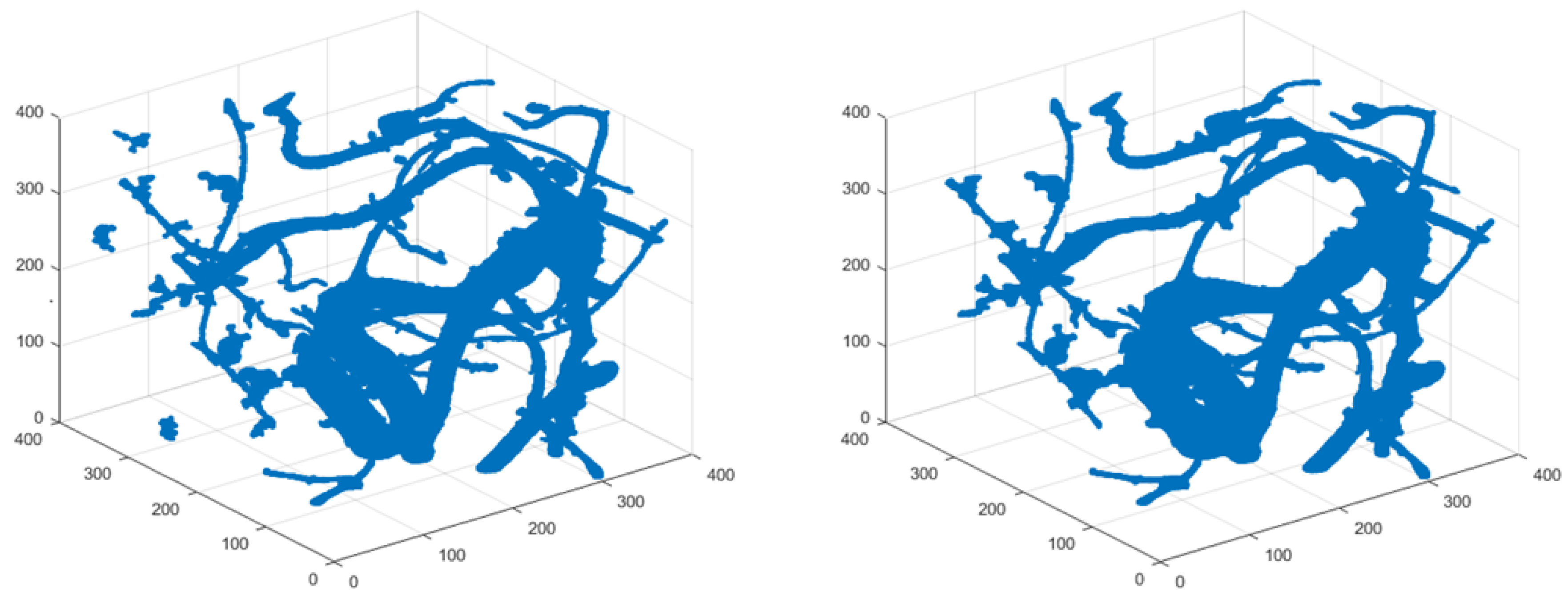
To illustrate the role and importance of different post-processing approaches in root-system reconstruction, we show the effects of different steps in post-processing on root-system reconstruction of cassava based on high-resolution 3D X-ray CT data. Typical cassava root information can be found from the Cassava Source Sink project at http://www.biochemie.nat.uni-erlangen.de/Cassava/index.html. The post-processing procedure after segmentation is described as follows. First, filter the components by three criteria: (1) volume, which is the number of voxels; (2) extent, which is the ratio of the component volume to the volume of its bounding box; and (3) principal length ratio, which is the ratio of the maximum length of the three major axes to the minimum length. For each component, the three lengths obtained are the length (in voxels) of the major axes of the ellipsoid that have the same normalized second central moments as this component [42]. The identified root system before and after this filtering step is shown in Figure 1 to illustrate the effect of this post-processing step. A morphological closing operation (by 10 voxels) has also been applied. The component with the biggest volume and its neighboring components (within 30 voxels) were labeled as root. The identified root system before and after this post-processing step is shown in Figure 2.
After segmentation and post-processing, the next step is the extraction of phenotypes (especially root system architecture (RSA)) after root-system reconstruction. Root system architecture describes the spatial arrangement of roots within the soil and, by facilitating efficient nutrient and water uptake from the soil, is crucial in plant performance [12,28]. A range of RSA traits in both 2D and 3D can be extracted depending on researchers’ interests and purposes. For example, in one study to investigate the effects of soil on RSA and crop productivities, the extracted RSA traits for cultivars are root depth, width, total length, convex area, diameter, median root number, and crown root number [43]. A more complete review of 3D root system architecture can be found in Morris et al. [44]. Accurate extraction of RSA traits depends on previous segmentation and root-system reconstruction (post-processing) so all three issues are important for further downstream analysis such as linking extracted RSA traits to genotypes and environmental variables.
CT-scanning in a non-medical plant context usually involves scanning the root systems below ground, and leaf canopies above ground. Lafond et. al. present a nice review of relevant applications [7]. Detection of the plant seed directly is usually not a primary study goal, but new methods are emerging focusing on seed-soil contact areas [45]; in some studies the seed volume is accounted for in the model parameters when estimating root volumes and detecting first-order roots [17], and plants are usually scanned after the first 7–8 days of planting [46].
As stated above, data values from CT-scans are converted to grayscale intensity values that represent the different materials present in the scan. In a root segmentation analysis, these grayscale values represent both root and soil, along with other materials that are present at the time of scanning. The values represent each overlap, and are not good measures for identifying features by themselves [47]. Error in the analyses will most likely come from measurements at the root-soil border, or at regions were the intensity of the root itself varies from other regions. In developing the RooTrak software [48], Mairhofer et. al describe two philosophical approaches for root segmentation: top-down (detecting objects that are similar to a parent object) and bottom-up (refinement and grouping of similarly classed objects). Overall image quality is an important factor in the success of the segmentation process (as it is in most image analysis workflows); how each method handles the presence of water and other organic material in the soil is also important.
3. Existing Approaches
We provide a brief overview of the most recent literature on analytical approaches and tools that have been used in 3D X-ray CT imaging for medical applications or/and agricultural applications. Some approaches have been used only for medical applications, but they may be of use in plant phenotyping due to similar X-ray data structures shared in medical images and agricultural images. For a more through review of 3D vessel lumen segmentation approaches prior to 2009 see Lesage et al. [49]. Relevant mathematical details can be found in the Appendix.
3.1. Statistical Branch Tracking Based on Vesselness Measures
The aim of this section is to concisely summarize some approaches to the identification and tracking of root-like structures in imaging data. Vesselness is often conceptualized as the probability or likelihood that an image region contains a tubular structure. This probability or likelihood is calculated by a vesselness filter or function based on mathematical values derived from such a region. Multiple versions of vesselness enhancement filters were developed in Frangi et al. (1998) [50] using the eigenvectors of the Hessian to compute the likeliness of an image region to contain vessels or other image ridges. The work of Lo et al. (2010) [51] is an extension of Frangi et al. (1998) and vesselness measures used in Lo et al. (2010) actually come from Frangi et al. (1998). A vesselness measure is obtained on the basis of all eigenvalues of the Hessian, with two values for 2D pictures and three values for 3D X-ray CT image data [50].
This measure is used to find the roots based on their vesselness structure [52,53]. Frangi et al.’s method (1998) requires the calculation of three indexes based on eigenvalues of the Hessian, which can be viewed as a thresholding approach but based on the three indexes instead of original intensity values of the voxels. Its implementation is fast compared to more recently used approaches. Root analysis results using this approach were presented and discussed at a recent scientific conference [54].
Extending from Frangi et al. (1998), Lo et al. (2010) [51] use a voxel classification model based on k nearest neighbors (kNN) to distinguish airway tree from non-airway voxels for better understanding of chronic obstructive pulmonary disease (COPD). Lo et al.’s method (2010) has been used primarily for medical applications and has potential benefit for root phenotyping. Any classification-based appearance model such as theirs requires a training data set. However, the gold standard obtained by hand-tracing is unavailable. Thus, Lo et al. (2010) use an intensity-based region growing algorithm to obtain the manual segmentations needed, where both the seed point and thresholding value in the region growing procedure have to be determined manually. A high threshold value is used to obtain a conservative set and then a threshold value only slightly higher than what is commonly used by researchers to do the usual segmentation is adopted to obtain a set with a small proportion of false positives. The actual training set is a combination of these two data sets, after some morphological changes. Lo et al.’s approach (2010) identifies root systems by supervised classification instead of unsupervised segmentation after obtaining this training set.
With this manually identified training set using a region expansion algorithm, a kNN classifier is applied. The initial feature sets used in classification are mostly local image descriptors which consist of spatial derivatives up to and including the second order and measures calculated from the Hessian matrix, which are the eigenvalues, determinant, trace, and Frobenius norm. The features also include combinations of eigenvalues that measure tube, plate and blobness as discussed in Frangi et al. (1998) [50]. Similar to before, these measures are calculated at multiple scales. Sequential floating forward feature selection is used to find an optimal set of image descriptors and the final kNN classifier is constructed using the optimal combination of features and all training samples. With the constructed kNN classifier, for each voxel, researchers can estimate the posterior probability of membership in the airway class (versus not airway), given a set of optimal features [51].
It should be noted that in order to extract RSA, processing steps post-vesselness filtering are likely to be required. For example, vessel-like structures can be integrated to form a continuous root structure using graph-like approaches; see Schulz et al. (2013) [52] for more details. One can also apply a connected components analysis [55] to link disjoint tubular structures. Compared with Frangi et al.’s index-thresholding method (1998), Lo et al.’s method (2010) has multiple-step processing combining different methods (region growing, k-means classification et al., modified indexes from Frangi et al.’s method) to achieve good accuracy.
3.2. Bayesian Single Branch Tracking
Wang et al. (2012) [56] proposed a recursive Bayesian tracking technique (like [57]) and a cylindrical model (tubular structure) for single branch tracking. To our knowledge this has not yet been applied to the characterization of RSA. This Bayesian method is highly computationally-intensive compared with the single-step approach of Frangi et al. (1998) and the multiple-step approach from Lo et al. (2010). However, it does provide additional information in the form of probabilities of the existence of specific root tracks.
The posterior probability of a given hypothesis, i.e., track, is based on a state vector including the position, orientation, radius and intensity of each branch segment. Reference centerlines are provided by training data sets, and the distributions of radius changes and direction changes are modeled as prior information. Since branches usually decrease in size, two different standard deviations are estimated for positive and negative radius changes. The values of the posteriors are used to recognize the end of a segment according to a user-provided threshold. In this approach, branch detection is based on deviations from a single cylinder model and side flux (see Appendix for details). Prior to any modeling there is an initiation and preprocessing step which involves starting radii and starting directions for possible root structures.
Their overall algorithm after initialization and pre-processing is:
| Algorithm 1 Single Branch Tracking |
|
| Algorithm 2 Branching Detection |
|
3.3. Bayesian Tracking with Overlap of Intensities
The method presented in Schaap et al. (2007) [57] is designed for tracking and extraction of tubular structures when there are regions of varying intensities and these intensities overlap. This is true of root voxel intensities and intensities of other matter such as air and water. The structures of interest are assumed to be more homogeneous relative to background, which is commonly observed in 3D X-ray CT image data. Schaap et al.’s method (2017) was initially provided as a general approach to identifying tabular structures and the authors illustrated the use of the method for tracking the internal carotid artery from CT angiography data. Later applications of Schaap et al.’s method (2017) were mainly on 3D X-ray CT medical images, and there are no applications of their approach based on agricultural images. Schaap’s method allows imposing prior information on shape and appearance, and researchers can improve the performance of this approach with improved knowledge of shape and appearance and by modifying the prior specification to solve more flexible and general problems.
The overall Bayesian framework is to impose prior information on shape and appearance, calculate a likelihood based on a tubular model, and then conduct recursive estimation based on the posterior. See the Appendix for details.
A tube is modeled as a series of tube segments, and every segment is associated with a region of interest (ROI). By sampling around the ROI, two intensity measures are calculated which represent the similarity between the intensity distributions of the current and previous tube segments and between the inside and outside of the tube, respectively. These measures are used to determine whether a given voxel has been identified as part of the tube or not, and are updated iteratively as voxels are identified. This iterative approach is used in their approaches for tracking and extraction of tubular structures [57].
3.4. Tracking Based on A Constrained Geometric Model for Tabular Structures
The approach presented in Lesage et al. (2008) [58] is similar to those presented above [56,57]). It uses a constrained medial-based geometric model and a sampling scheme for selecting hypotheses/states, assuming differences in intensities between the structure of interest and the background. These methods have been used in X-ray CT medical imaging; to our knowledge they are yet to extend to RSA imaging. Adding geometric constraints to modeling, in general, is believed/expected to improve performance.
A tubular structure is represented by a collection of maximally included hyper-spheres; the sphere centers form the medial axis of the object and the radii allow for reconstruction of the object surface. During tracking, the model is iteratively updated by adding new sphere centers which lie on the surface of the preceding sphere (a connectivity constraint). Tracking proceeds via iterative stochastic Bayesian filtering, i.e., candidate sphere centers and radii are recursively considered, evaluated, and then used to update the current model. The evaluation process involves measures of gradient flow and the alignment of the sphere surface with the image gradient vector field. Details are available in the Appendix.
4. 2D to 3D Structure Determination
These two approaches analyze 2D images and combine these images to create a 3D image. They have been presented recently in the medical imaging literature but may contribute to the development of novel approaches to X-ray CT root imaging.
4.1. cryoSPARC for Cyro-EM 3D Structure Estimation
Single-particle cryo-electron microscopy (cryo-EM), given appropriately prepared samples, has enabled near-atomic-resolution structure determination of scientifically important proteins [59]. Although tens of thousands of high-resolution images can be produced in 24 to 48 h, the analysis of these images can be much more resource intensive. Punjani et al. (2017) [60] present an approach to processing cryo-EM image data in two steps. The first step is unsupervised extraction of a rough, approximate structure and the second step is a high-resolution refinement of this structure. Although this approach was developed for cyro-EM image data, the algorithm and idea may be useful in analyzing other types of images including X-ray CT images.
In the first step, stochastic gradient descent (SGD) is used to quickly identify a low-resolution 3-D structure that is consistent with the available set of 2D images (of which there are tens of thousands). This identification is based on the probability of observing a particular 2D image given a particular 3D model, and iteratively updating the 3D model to maximize this probability. The SGD is randomly initialized by selecting a mini-batch of 2D images, assigning them random pose angles, and using them to reconstruct an initial 3D volume.
Usually with cryo-EM the noise comes from the contrast transfer function or CTF, i.e., from the shot and readout noises of the microscope. The authors provide an augmented approximate maximum a posteriori (MAP) estimate of this noise based on a decaying running average, which they include in the error of the 3D model. For details see [60] and the Appendix.
In the second step, once the SGD has been used to generate an estimate of the volume to medium resolution, an expectation-maximization (EM) algorithm is used to refine this estimate to high resolution. The expensive part is the E step in which each 2D image is aligned over 3D orientations and 2D translations to the current estimate of each 3D structure. This is done by branch-and-bound search, i.e., calculating upper and lower bounds of the search criterion and then using these to exclude regions of the search space at each iteration. For efficiency, the branch and bound search uses an empirical (prior) initial sampling of poses.
4.2. KNOSSOS and ElektroNN2
Dorkenwald et al. (2017) [61] present a method developed primarily for neurite reconstruction from EM imaging data. Their approach uses skeleton reconstructions from KNOSSOS (https://knossostools.org/)(V5.1, Max Plank Institute for Medical Research, Hiedelberg, Germany) as input to ElektroNN2 (http://elektronn.org/) (Max Plank Institute for Medical Research, Hiedelberg, Germany), a software the authors developed in Python Theano for recursive 3D CNN. ElektroNN2 builds volume reconstructions from serial block-face EM data sets. This software has not be applied to root imaging, but the method may extend to the identification of ‘neurite-like’ root structures.
The conversion of skeletons to volume reconstructions is done by training a recursive 3D CNN model to predict barrier regions between neurites, with a ray casting approach where CNN prediction fails. CNN training data for one data set can be used to pre-train a network for a different neurite data set, hence reducing the amount of training data required.
The discovery of synapses and other ultrastructural objects is done by exploiting co-occurrence and training a multiclass CNN. The resulting ultrastructural objects are then mapped to neurites by whether or not the objects are located on the boundary of a neurite skeleton. Once this mapping is complete, a random forest [62] on CNN-extracted features (i.e., ultrastructural objects mapped to neurites) is used to classify local environments as parts of a dendrite or axon or other neural structure.
5. Other Recent Approaches
We note here briefly two techniques that are receiving considerable attention in the scientific imaging community, namely, deep learning and graph-based segmentation.
5.1. Deep Learning
Artificial Neural Networks (ANNs), and their “Deep” (many hidden layers) variants (Deep Neural Networks) are very efficient methods for analyzing and classifying large quantities of images with high accuracy [63]. These networks have been used in fields as broad as self-driving cars for detecting pedestrians [64], to automatically detecting arrhythmia conditions [65] in cardiac patients and electrocardiography (ECG/EKG) applications [66]. As we noted above, convolutional neural networks have been used to detect ‘root-like’ structures in brain imaging and may extend to X-ray CT imaging of plant roots. One drawback of deep learning is the need for large volumes of annotated training data, data which is not always available.
5.2. Graph-Based Segmentation
Graph-based segmentation methods treat an image as a graph and conduct segmentation by graph cuts [67]. These methods define a link between dissimilar pixels to be low cost and a link between similar pixels to be high cost. In separating the graph into segments according to the values of this cost function, similar pixels are more likely to be in the same segment. Graph-based methods have been used in analyzing X-ray CT images for segmentation and quantitative analysis of porous materials [68] and airway wall structure [69]. Graph-based methods have also been used for root-phenotyping based on 2D images [70,71] and likely extend to root phenotyping based on 3D X-ray images.
6. Available Computational Tools
Although most 3D CT-image-based root-system analysis approaches do not have corresponding software available, there are still some software tools for root system tracking based on 3D CT images.
6.1. ImageJ and Root1
ImageJ is a public domain tool for scientific image analysis [72] that is freely available from the US National Institute of Health (NIH) (https://imagej.nih.gov/ij/) website. The ImageJ software is written in the Java programming language, runs on many popular desktop computer operating systems, and offers a very powerful plug-in model for extending the capabilities of the base system [73].
The Root1 macro [74,75] is a recently developed plug-in for ImageJ that provides users with tools and semi-automated analysis protocols for working with micro-Computed Tomography (CT) images. The basic set of tools, and the general workflow, of the Root1 software is (1) Normalization of the input images; (2) Identification of putative roots; (3) Artificial expansion of volumetric objects; (4) Removal of partial volume effects; (5) Application of thresholding and filtering methods; (6) Extraction of roots; and lastly the analysis of the extracted root skeletons.
An advantage of Root1 is that it automates many of the repetitive, labor-intensive tasks that a researcher would have to perform by hand. Root1’s automated macro can be easily customized to match a sample’s unique conditions, so researchers can tweak and adjust parameters to suit their needs. A disadvantage is that as of this writing it does not support parallel processing, and large, high-resolution, datasets could take some time to process.
6.2. RooTrak
RooTrak is a free software for recovering root architecture from X-ray micro-Computed Tomography (CT) image data developed by Mainhofer et al. (2013) [47]. Information about this computer vision group at the University of Nottingham can be found at http://www.cs.nott.ac.uk/~psztpp/styled-6/index.html.
X-ray attenuation values of roots and non-roots may overlap, and the attenuation values of root material have their own inherent variability. Any successful root identification method must both explicitly target root material and be able to adapt to local changes in root properties [47]. RooTrak meets these requirements by combining a level set method with a visual tracking framework to segment a variety of plant roots from soil in X-ray (CT) images.
The key idea in RooTrak tracking is to view a 3D image as a sequence of parallel 2D images, through which 3D root objects appear to move as the x-y cross-sections are traversed along the z-axis of the image stack (except the upward-growing (plagiotropic) branches). The extended software tool produces more complete descriptions of plant root structure and supports more accurate computation of architectural traits including the tracking of plagiotropic branches. RooTrak exploits multiple, local models of root appearance, each built while tracking a specific segment, to identify new root material. The advantage of Rootrak is that it requires minimal user interaction and is able to adapt to changing root density estimates [47].
6.3. VG Studio Max
VG Studio Max software allows for 3D X-ray CT analysis with the add-on modules ‘Coordinate measurement’ (Advanced surface determination) and ‘Wall thickness analysis’. Analyzing root systems using VG Studio Max is not automatic and includes multiple user-driven steps. Most steps need manual monitoring and judgment, and some steps need additional data processing in MATLAB. An example of using VG Studio Max in analyzing roots can be found in Pfeifer et al. (2015) [25].
6.4. Volume Player Plus (VPP) and Modular Algorithms for Volume Images (MAVI)
These two commercial software tools are available from Fraunhofer Development Center X-ray Technology (EZRT). Although these softwares were developed for EZRT’s CT setup and facilities, they can also be used to analyze 3D CT images from other CT facilities. An example of using these tools for root analysis based on 3D CT images can be found in Metzner et al. [26].
6.5. Digital Imaging of Root Traits (DIRT)
DIRT measurements are inspired by the ‘shovelomics’ standard for root excavation. In the shovelomics protocol, researchers excavate a root at a radius of 20 cm around the hypocotyl and 20 cm below the soil surface. After excavation, the shoot is separated from the root 20 cm above the soil level and washed in water containing mild detergent to remove soil. Then the washed root is placed on a phenotyping board consisting of a large protractor to measure dominant root angles with the soil level at depth intervals and marks to score length and density classes of lateral roots. Observed traits include angle, number, density, and diameter. The shovelomics phenotyping method is not image-based as researchers manually measure root traits [3].
DIRT extended shovelomics (manual trait estimation) by taking digital images. Similar to shovelomics, the root crown is excavated, washed in water, and then placed on a board to enable trait estimation. Instead of manually measuring traits, digital images are taken using the DIRT imaging protocol. Then users of DIRT can compute over 70 root traits directly from these images. DIRT is a high-throughput RSA trait computation platform which makes RSA trait computation available to the community with some simple button clicks. It is accessible at http://dirt.iplantcollaborative.org/ and hosted on the CyVerse cyber-infrastructure using high-throughput grid computing resources from the Texas Advanced Computing Center (TACC) [76].
DIRT works for 2D RGB (visible-light) images instead of 3D X-ray CT images. There have been multiple software tools available for root analysis based on 2D RGB images. A comprehensive overview can be found at http://plant-image-analysis.org.
7. Discussion and Conclusions
We present an overview of recent statistical and computational approaches that have or may be applicable to root analysis based on 3D X-ray CT image data as a way to introduce this area of research to the scientific community.
With the rapid development in X-ray CT technology and generation of massive 3D CT scanning data, we expect future research will focus on proposing automatic high-throughput approaches and tools with the capability of handling massive amounts of data and parallel computation. An increased use of deep learning approaches in root analysis is expected since deep learning has seen great success in analyzing medical 3D X-ray images.
One issue in machine learning in general, and in deep learning specifically, is access to relatively large amounts of labeled training data (ground-truth). An approach to addressing this issue is to use simulated data to improve accuracy in root image analysis pipelines [24]. Improving structural root system simulation and how to combine simulated data with real data in root system analysis are open research questions for further study.
In addition to root-phenotyping based on 3D X-ray CT images, destructive root phenotyping approaches such as shovelomics and DIRT may be used to generate ground truth data. X-ray CT data sets with ground truth obtained by shovelomics and DIRT may be used as the benchmark data set to evaluate the performance of algorithms. Another advantage of this X-ray CT data with ground truth labels is that it can be used for supervised deep learning approaches. This type of ground-truth data set could be more costly than simulation methods for generating ground truth data as discussed in the previous paragraph, but it may avoid simulation biases and the obtained data set may be more realistic than a simulated data set.
In terms of computational demand and estimation accuracy, different methods have different characteristics. Direct/Naive implementations of segmentation approaches from computer vision as reviewed above (including thresholding, region growing, clustering, and nearest neighbors) have the lowest computational costs but performance may not be satisfactory. Combined multiple-step approaches will improve performance at the cost of longer computing times. The existing approaches that we have reviewed in more detail (in Section 3, Section 4, Section 5 and Section 6) should have better performance than basic segmentation approaches, although this has yet to be demonstrated for some approaches. Frangi’s method (1998), as a thresholding approach based on indexes calculated from the eigenvalues of the Hessian, is fastest and preferred by some researchers due to its computational speed and simplicity. Lo et al.’s method (2010) is multiple-step, combining nearest neighbor clustering, region expansion approach and the use of modified vesselness indices. The Bayesian approaches reviewed are expected to require more computational resources but do allow the researcher to include domain knowledge of the structure of interest, geometric constraints, and appearance in the prior to achieve better performance.
Recent technologies have enabled parallel computation by GPU or computational clusters (Unix server). Parallel computing distinguishes an approach/algorithm’s computational complexity/amount and its computational time. An approach may have a large requirement for computational amount/complexity but a small computational time if the algorithm allows for a parallel implementation. In contrast, a sequential computing method may have a relatively low requirement for computational resources but still needs a long time to run due to its inability to execute in parallel. We expect parallel computation and crowd computing to improve our current ability to process and analyze root phenotyping images. In view of these facts, we describe two approaches that (1) represent a 3D object as multiple 2D images; (2) analyze the 2D images in parallel and then (3) combine these images to create a 3D image of the original object. These two approaches (cyroSPARC and KNOSSO-ElectroNN) were originally developed for medical imaging but have potential for root phenotyping given their parallel implementations which reduce runtime and their demonstrated accuracy on cyro-electron microscopy images.
Although this review is mainly focused on analytical approaches either used or proposed in root phenotyping, we have presented brief descriptions of available computational software for root phenotyping. One crucial question/limitation in X-ray CT root phenotyping is the lack of a well-established publicly-available software pipeline. Thus, publicly-available software development remains a bottleneck and future research in developing software (which can correspond to existing or novel approaches) are motivated and necessary to facilitate and improve non-destructive root phenotyping.
Author Contributions
Z.X. and J.C. conceived of the manuscript; Z.X., C.V. and J.C. contributed to the writing of the manuscript.
Acknowledgments
We thank Stefan Gerth of Fraunhofer IIS for helpful discussions.
Conflicts of Interest
The authors declare no conflict of interest.
Abbreviations
The following abbreviations are used in this manuscript:
| 2D | Two Dimension |
| 3D | Three Dimension |
| ANN | Artificial Neural Network |
| CNN | Convolutional Neural Network |
| COPD | Chronic Obstructive Pulmonary Disease |
| CT | Computed Topology |
| CTF | Contrast Transfer Function |
| CTN | Computed Topology Number |
| DIRT | Digital Imaging of Root Traits |
| DNN | Deep Neural Network |
| EM (algorithm) | Expected-Maximum (algorithm) |
| EM (image) | Electronic Microscopic (image) |
| MAP | Maximum A Posteriori |
| MAVI | Modular Algorithms for Volume Images |
| MCMC | Markov Chain Monte Carlo |
| MRI | Magnetic Resonance Imaging |
| NIH | National Institute of Health |
| NN | Nearest Neighbor |
| RGB (image) | Red Green Blue (image) |
| RSA | Root Structure Architecture |
| SGD | Stochastic Gradient Descent |
| TACC | Texas Advanced Computing Center |
| VPP | Volume Player Plus |
Appendix A. Methodological Details
Appendix A.1. Statistical Branch Tracking Based on Vesselness Measures
As presented in Frangi et al. (1998) [50], is inferred by first calculating the Hessian matrix at based on its neighborhood. Denote as the Hessian matrix of the image computed at at scale s. Then the eigenvalues and eigenvectors of this Hessian matrix are calculated. Denote as the eigenvalue with the k-th smallest magnitude. Denote its corresponding eigenvector as . For 3D X-ray data, and indicates the direction along the vessel for a vessel structure. Then Frangi et al. (1998) summarize the relationships that must hold between eigenvalues of the Hessian for the detection of different structures. Different patterns of an image around a point can be measured by the eigenvalues of its Hessian matrix H. Denote , , , (N usually small), and let indicate the sign of the value. Then orientation patterns around the point are summarized as follows: For 2D images, when are respectively , , , , , the orientation patterns are identified, respectively, as “noisy, no preferred direction”, “tabular structure (bright)”,“tabular structure (dark)”,“blob-like structure (bright)”,“blob-like structure (dark)”. For 3D images, when are respectively , , , , , and , the orientation patterns are identified, respectively, as “noisy, no preferred direction”, “plate-like structure (bright)”, “plate-like structure (dark)”, “tabular structure (bright)”, “tabular structure (dark)”, “blob-like structure (bright)” and “blob-like structure (dark)”.
For 3D images, Frangi et al. (1998) construct three indexes: , , and . Then the vesselness function is defined by combining these three indexes, i.e.,
where , and c are parameters controlling the sensitivity of the line filter to the measures , and . This vesselness function is analyzed at different scales s, we integrate the vesselness measure at different scales to obtain a final estimate of the vesselness:
where and are the maximum and minimum scales at which we expect to find relevant structures.
Appendix A.2. Bayesian Single Branch Tracking
As described in Wang et al. (2012) [56], the posterior probability of a given hypothesis, i.e., track, is based on a state vector including the position , orientation , radius and intensity of each branch segment. The recursive Bayes rule employed is
A Markovian process is assumed so the transition prior may be expressed as
The change in radius and angle between and are calculated at each sample point extracted along the reference centerline. This approach assumes that and with parameters learned from reference centerlines (prior knowledge or empirical). Here represents the mean value (mean change in radius or mean angle) and represents the standard deviation (standard deviation of mean change in radius or standard deviation of angles). Since branches usually decrease in size, two different standard deviations are estimated for positive and negative radius changes.
The likelihood represents a cylindrical geometrical model and minimal flux, with uniformly distributed points created at the outer edge of the cylinder’s cross-sections and , with i indexing the points in a cross-section and j indexing the points in a longitudinal direction. So
with as the gradient vector at point , as the inward radial direction, and as the scalar product. Then the likelihood function is
where is the sigmoid function and the Normal is used to ensure that the inner intensities of the model resemble those of the tubular structure. Branch detection is based on deviations from the single cylinder model and side flux. A side is represented as a point set where k and j are indices of points in the cross-sectional and longitudinal directions of the cylinder, and m are the max number of points in these directions, and i is the start position of the side. These lead to side sets defined by as . So side flux can be stated as
with
In this formulation is the gradient vector at and is the inward radial direction. This is matched with a metric of intensity differences between points s and on opposite sides of the cylinder to get a measure whose minimum is used as an indication of a branching candidate, e.g.,
Appendix B. Bayesian Tracking with Overlap of Intensities
As described in Schaap et al. [57], a tube segment at iteration t is described by its location , orientation , radium , intensity , and intensity variance . These form a state vector , so the entire tube can be described by . Every segment is associated with a region of interest (ROI) U defined by and of with representing the image intensities within U. Denote as the set of spatial coordinates within the tube and be similar coordinates in a band around the tube.
The distributions and are constructed by sampling with nearest-neighbor interpolation from the ROI. Given and the likelihood is
where is a spatial prior to prevent loops, is a prior on expected radii, and the two intensity measures are designed to reflect the similarity between the intensity distributions of the current and previous tube segments and between the inside and outside of the tube, respectively. In other words,
The estimates come from the histogram of , and moderate the influence of the two pieces. The function D is a metric of distributional similarity. For they store a spatial map of whether each voxel has been identified as part of the tube or not, with , and update after each iteration. The prior reflects an average of this map over the ROI, or
The posterior distribution can now be estimated by the following recursion
where the transition prior is Markovian and factored as
assuming no transition model for and all intensities are equally probable.
Appendix B.1. Tracking Based on A Constrained Geometric Model for Tabular Structures
As presented in Lesage et al. (2008) [58], a tubular structure is represented by a collection of maximally included hyper-spheres of centers and radii . A non-branching structure is represented as or, equivalently, where the radii and axis directions appear as linked variables: and . A center at iteration t sets the radius and direction at iteration .
Tracking proceeds via an iterative stochastic Bayesian filter, i.e., a first-order hidden Markov model (HMM) and a Monte-Carlo (MC) approximation of the posterior by a weighted set of discrete samples . So at iteration t consider all candidate as discrete locations at distances of . A candidate retrospectively fixes and according to the model above. Associated weights are
The set forms a ‘distribution’ from which a new set is found by importance sampling with weights normalized to sum to one.
The likelihood can be represented as , where measures gradient flow through the surface of sphere of radius with center , i.e.,
where is the image gradient and is the unit normal to . This quantifies the alignment of the sphere surface with the image gradient vector field. Two additional variables are important in tracking: (1) The variable is the response of the morphological erosion by the sphere at point , i.e.,
where is the image intensity at location z; (2) The variable is a difference term that counterbalances the shrinkage effect of and favors points with high intensity and location far from (near the centerline), i.e.,
The prior treats the radius and direction as independent variables, i.e.,
with both distributions learned from manually segmented images, i.e., empirical histograms of radius variation and direction variation . These histograms are used directly to evaluate both pieces of the prior.
Appendix B.2. cryoSPARC for cryo-EM 3D Structure Estimation
In the first step, stochastic gradient descent (SGD) is used to quickly identify a low-resolution 3-D structure that is consistent with the available set of 2D images (of which there are tens of thousands). The objective function is a log posterior probability distribution over K 3D densities given N 2D particle images , with the format,
Since the posterior is a marginal probability with marginalization over unknown variables, we can re-express the above in more detail, i.e., and . Hence,
The integrand reflects the probability of observing a particular 2D image given a particular pose and 3D model . The pose is expressed as a pair denoting the 3D orientation of the object and the 2D translation of the object within the object image. can be expressed in the Fourier domain as well (which we omit here). Stochastic gradient descent (SGD) is used to iteratively update the parameters , which are represented as voxels of density on 3D grids. The first step is to take the gradient with respect to each structure , which can be approximated using random subsampling via mini batches of size M of 2D images at each iteration. Then the update at the current iteration is computed by scaling the current gradient, denoted as , with a step-size and combining this linearly with the previous update with a ratio determined by . In other words,
The step size is intended to reflect the second-order curvature of the objective function . The maximum curvature over all dimensions in Fourier space is used as the inverse step-size for each structure. The computation of the approximate Hessian is done over the mini batch within each iteration and re-uses some of the computation required for the gradient ; the re-use provides some computational efficiencies.
Usually with cryo-EM the noise comes from the contrast transfer function or CTF, i.e., from the shot and readout noises of the microscope. The authors provide an augmented approximate maximum a posteriori (MAP) estimate of this noise based on decaying running average, which they include in the error of the 3D model.
In the second step, once the SGD has been used to generate an estimate of the volume to medium resolution, an EM algorithm is used to refine this estimate to high resolution. The expensive part is the E step in which each 2D image is aligned over 3D orientations and 2D translations to the current estimate of each 3D structure. This is done by branch-and-bound search, i.e., calculating upper and lower bounds of the search criterion and then using these to exclude regions of the search space at each iteration. The intuition behind the derivation is that the error is a sum of terms in which each Fourier coefficient contributes independently, and only coefficients with sufficient power matter are retained. This bound is used to discard regions of the space of 3D poses and 2D shifts. Regions of this space are represented using a cartesian grid in axis-angle space for 3D and second grid in 2D space of pixel shifts. An upper limit is set on the number of candidate poses that can remain after each iteration of search.
References
- Tollner, E.; Verma, B.; Cheshire, J. Observing soil-tool interactions and soil organisms using X-ray computer tomography. Trans. Am. Soc. Agric. Eng. 1987, 30, 1605–1610. [Google Scholar] [CrossRef]
- Dutilleul, P.; Lafond, J. Branching and Rooting Out with a CT Scanner: The Why, the How, and the Outcomes, Present and Possibly Future; Frontiers Media: Lusanne, Switzerland, 2016. [Google Scholar]
- Trachsel, S.; Kaeppler, S.; Brown, K.; Lynch, J. Shovelomics: High throughput phenotyping of maize (Zea mays L.) root architecture in the field. Plant Soil 2010, 341, 75–87. [Google Scholar] [CrossRef]
- Chen, X.; Ding, Q.; Blaszkiewicz, Z.; Sun, J.; Sun, Q.; He, R.; Li, Y. Phenotyping for the dynamics of field wheat root system architecture. Sci. Rep. 2017, 7. [Google Scholar] [CrossRef] [PubMed]
- Downie, H.; Adu, M.; Schmidt, S.; Otten, W.; Dupuy, L.; White, P.; Valentine, T. Challenges and opportunities for quantifying roots and rhizosphere interactions through imaging and image analysis. Plant Cell Environ. 2015, 38, 1213–1232. [Google Scholar] [CrossRef] [PubMed]
- Roose, T.; Keyse, S.; Daly, K.; Carminati, A.; Otten, W.; Vetterlein, D.; Peth, S. Challenges in imaging and predictive modeling of rhizosphere processes. Plant Soil 2016, 407, 9–38. [Google Scholar] [CrossRef]
- Lafond, J.; Han, L.; Dutilleul, P. Concepts and analyses in the CT scannning of root systems and leaf canopies: A timely summary. Front. Plant Sci. 2015, 6, 1111. [Google Scholar] [CrossRef] [PubMed]
- Wachsman, G.; Sparks, E.; Benfey, P. Genes and networks regulating root anatomy and architecture. New Phytol. 2015, 208, 26–38. [Google Scholar] [CrossRef] [PubMed]
- Lynch, J. Root phenes for enhanced soil exploration and phosphorus acquisition: Tools for future crops. Plant Physiol. 2011, 156, 1041–1049. [Google Scholar] [CrossRef] [PubMed]
- Gumayao, R.; Chin, J.; Pariasca-Tanaka, J.; Pesaresi, P.; Catausan, S.; Dalid, C.; Slamet-Loedin, I.; Tecson-Mendoza, E.; Wissuwa, M.; Heuer, S. The protein kinase Pstol1 from traditional rice confers tolerance of phosphorus deficiency. Nature 2013, 488, 535–539. [Google Scholar] [CrossRef] [PubMed]
- Ahmed, S.; Naugler Klassen, T.; Keyes, S.; Daly, M.; Jones, D.; Mavrogordato, M.; Sinclair, I.; Roose, T. Imaging the interaction of roots and phosphate fertiliser granules using 4D X-ray tomography. Plant Soil 2015, 401, 125–134. [Google Scholar] [CrossRef]
- Rich, S.; Watt, M. Soil conditions and cereal root system architecture: Review and considerations for linking Darwin and Weaver. J. Exp. Bot. 2013, 64, 1193–1208. [Google Scholar] [CrossRef] [PubMed]
- Koevoets, I.; Venema, J.; Elzenga, J.; Testerink, C. Roots Withstanding their Environment: Exploiting Root System Architecture Responses to Abiotic Stress to Improve Crop Tolerance. Front. Plant Sci. 2016, 7, 1335. [Google Scholar] [CrossRef] [PubMed]
- McMichael, B.; Burke, J. Soil temperature and root growth. HortScience 1998, 33, 947–951. [Google Scholar]
- Rey, T.; Schornack, S. Interactions of beneficial and detrimental root-colonizing filamentous microbes with plant hosts. Genome Biol. 2013, 14, 121. [Google Scholar] [CrossRef] [PubMed]
- Hacquard, S.; Kracher, B.; Hiruma, K.; Münch, P.; Garrido-Oter, R.; Thon, M.; Weimann, A.; Damm, U.; Dallery, J.F.; Hainaut, M.; et al. Survival trade-offs in plant roots during colonization by closely related beneficial and pathogenic fungi. Nat. Commun. 2016, 7, 11362. [Google Scholar] [CrossRef] [PubMed]
- Han, L.; Dutilleul, P.; Prasher, S.O.; Beaulieu, C.; Smith, D.L. Assessment of common scab-inducing pathogen effects on potato underground organs via computed tomography scanning. Phytopathology 2008, 98, 1118–1125. [Google Scholar] [CrossRef] [PubMed]
- Sturrock, C.J.; Woodhall, J.; Brown, M.; Walker, C.; Mooney, S.J.; Ray, R.V. Effects of damping-off caused by Rhizoctonia solani anastomosis group 2-1 on roots of wheat and oil seed rape quantified using X-ray Computed Tomography and real-time PCR. Front. Plant Sci. 2015, 6, 461. [Google Scholar] [CrossRef] [PubMed]
- McNear, D., Jr. The Rhizosphere—Roots, Soil and Everything In Between. Nat. Educ. Knowl. 2013, 4, 1. [Google Scholar]
- Philippot, L.; Raaijmakers, J.; Lemanceau, P.; van der Putten, W. Going back to the roots: The microbial ecology of the rhizosphere. Nat. Rev. Microbiol. 2013, 11, 789–799. [Google Scholar] [CrossRef] [PubMed]
- Stringlis, I.; Proietti, S.; Hickman, R.; Van Verk, M.; Zamioudis, C.; Pieterse, C. Root transcriptional dynamics induced by beneficial rhizobacteria and microbial immune elicitors reveal signatures of adaptation to mutualists. Plant J. 2018, 93, 166–180. [Google Scholar] [CrossRef] [PubMed]
- Piñeros, M.; Larson, B.; Shaff, J.; Schneider, D.; Falcão, A.; Yuan, L.; Clark, R.; Craft, E.; Davis, T.; Pradier, P.; et al. Evolving technologies for growing, imaging and analyzing 3D root system architecture of crop plants. J. Integr. Plant Biol. 2016, 58, 230–241. [Google Scholar] [CrossRef] [PubMed]
- Balduzzi, M.; Binder, B.; Bucksch, A.; Chang, C.; Hong, L.; Iyer-Pascuzzi, A.; Pradal, C.; Sparks, E. Reshaping Plant Biology: Qualitative and Quantitative Descriptors for Plant Morphology. Front. Plant Sci. 2017, 3, 117. [Google Scholar] [CrossRef] [PubMed]
- Lobet, G.; Koevoets, I.; Noll, M.; Meyer, P.; Tocquin, P.; Pages, L.; Perilleux, C. Using a Structural Root System Model to Evaluate and Improve the Accuracy of Root Image Analysis Pipelines. Front. Plant Sci. 2017, 8, 447. [Google Scholar] [CrossRef] [PubMed]
- Pfeifer, J.; Kirchgessner, N.; Colombi, T.; Walter, A. Rapid phenotyping of crop root systems in undisturbed field soils using X-ray computed tomography. Plant Methods 2015, 11, 41. [Google Scholar] [CrossRef] [PubMed]
- Metzner, R.; Eggert, A.; Dusschoten, D.; Pflugfelder, D.; Gerth, S.; Schurr, U.; Uhlmann, N.; Jahnke, S. Direct comparison of MRI and X-ray CT technologies for 3D imaging of root systems in soil: potential and challenges for root trait quantification. Plant Methods 2015, 11, 17. [Google Scholar] [CrossRef] [PubMed] [Green Version]
- Sharma, N.; Aggarwal, L. Automated medical image segmentation techniques. J. Med. Phys. 2010, 35, 3–14. [Google Scholar] [CrossRef] [PubMed]
- Lynch, J.; Brown, K. New roots for agriculture: exploiting the root phenome. Philos. Trans. R. Soc. Lond. B Biol. Sci. 2012, 367, 1598–1604. [Google Scholar] [CrossRef] [PubMed]
- Ginat, D.; Gupta, R. Advanced in Computed Tomography Imaging Technology. Annu. Rev. Biomed. Eng. 2014, 16, 431–453. [Google Scholar] [CrossRef] [PubMed]
- Larobina, M.; Murino, L. Medical Image File Formats. J. Digit. Imaging 2014, 27, 200–206. [Google Scholar] [CrossRef] [PubMed]
- Bryant, J.; Drage, N.; Richmond, S. CT Number Definition. Radiat. Phys. Chem. 2012, 81, 358–361. [Google Scholar] [CrossRef]
- Kalender, W. Computed Tomography; Publicis MCD Verlag: Oslo, Norway, 2000. [Google Scholar]
- Tjong, W.; Kazakia, G.J.; Burghardt, A.J.; Majumdar, S. The effect of voxel size on high-resolution peripheral computed tomography measurements of trabecular and cortical bone microstructure. Med. Phys. 2012, 39, 1893–1903. [Google Scholar] [CrossRef] [PubMed]
- Christiansen, B.A. Effect of micro-computed tomography voxel size and segmentation method on trabecular bone microstructure measures in mice. Bone Rep. 2016, 5, 136–140. [Google Scholar] [CrossRef] [PubMed]
- Downie, H.; Holden, N.; Otten, W.; Spiers, A.J.; Valentine, T.A.; Dupuy, L.X. Transparent soil for imaging the rhizosphere. PLoS ONE 2012, 7, e44276. [Google Scholar] [CrossRef] [PubMed]
- Mooney, S.; Pridmore, T.; Helliwell, J.; Bennett, M. Developing X-ray Computed Tomography to non-invasively image 3-D root systems architecture in soil. Plant Soil, 2012, 352, 1–22. [Google Scholar] [CrossRef]
- Gonzalez, R.; Woods, R. Digital Image Processing, 4th ed.; Pearson: London, UK, 2017. [Google Scholar]
- Gonzalez, R.; Woods, R.; Eddins, S. Digital Image Processing Using MATLAB, 2nd Edition; McGraw Hill India: New York, NY, USA, 2010. [Google Scholar]
- Solomon, C.; Breckon, T. Fundamentals of Digital Image Processing; Wiley-Blackwell: Hoboken, NJ, USA, 2011. [Google Scholar]
- Wang, H.; Mossa, R.; Chen, X.; Stanley, R.J.; William, V.; Stoecker, W.V.; Celebi, M.E.; Malters, J.M.; Grichnik, J.M.; Marghoob, A.A.; et al. Modified watershed technique and post-processing for segmentation of skin Lesions in dermoscopy images. Comput. Med. Imaging Graph. 2011, 35, 116–120. [Google Scholar] [CrossRef] [PubMed]
- Lai, M. Deep Learning for Medical Image Segmentation. arXiv, 2015; arXiv:1505.02000v1. [Google Scholar]
- Zelditch, M.; Swiderski, D.; Sheets, H.; Fink, W. Geometric Morphometrics For Biologists: A Primer; Elsevier Academic Press: New York, NY, USA, 2004. [Google Scholar]
- Rogers, E.; Monaenkova, D.; Mijar, M.; Nori, A.; Goldman, D.; Benfey, P. X-Ray computed tomography reveals the response of root system architecture to soil texture. Plant Physiol. 2016, 171, 2028–2040. [Google Scholar] [CrossRef] [PubMed]
- Morris, E.; Griffiths, M.; Golebiowska, A.; Mairhofer, S.; Burr-Hersey, J.; Goh, T.; von Wangenheim, D.; Atkinson, B.; Sturrock, C.; Lynch, J.; et al. Shaping 3D Root System Architecture. Curr. Biol. 2017, 27, R919–R930. [Google Scholar] [CrossRef] [PubMed]
- Blunk, S.; Malik, A.H.; de Heer, M.I.; Ekblad, T.; Bussell, J.; Sparkes, D.; Fredlund, K.; Sturrock, C.J.; Mooney, S.J. Quantification of seed-soil contact of sugar beet (Beta vulgaris) using X-ray Computed Tomography. Plant Methods 2017, 13, 71. [Google Scholar] [CrossRef] [PubMed]
- Subramanian, S.; Han, L.; Dutilleul, P.; Smith, D.L. Computed tomography scanning can monitor the effects of soil medium on root system development: An example of salt stress in corn. Front. Plant Sci. 2015, 6, 256. [Google Scholar] [CrossRef] [PubMed]
- Mairhofer, S.; Zappala, S.; Tracy, S.; Sturrock, C.; Bennett, M.J.; Mooney, S.J.; Pridmore, T.P. Recovering complete plant root system architectures from soil via X-ray μ-Computed Tomography. Plant Methods 2013, 9, 8. [Google Scholar] [CrossRef] [PubMed]
- Mairhofer, S.; Zappala, S.; Tracy, S.R.; Sturrock, C.; Bennett, M.; Mooney, S.J.; Pridmore, T. RooTrak: Automated recovery of three-dimensional plant root architecture in soil from x-ray microcomputed tomography images using visual tracking. Plant Physiol. 2012, 158, 561–569. [Google Scholar] [CrossRef] [PubMed]
- Lesage, D.; Angelini, E.; Bloch, I.; Funka-Lea, G. A review of 3D vessel lumen segmentation techniques: Models, features, and extraction schemes. Med. Image Anal. 2009, 13, 819–845. [Google Scholar] [CrossRef] [PubMed]
- Frangi, A.; Niessen, Q.; Vincken, K.; Viergever, M. Multiscale vessel enhancement filtering. In MICCAI’98. MICCAI 1998; Lecture Notes in Computer Science; Wells, W., Colchester, A., Delp, S., Eds.; Springer: Berlin/Heidelberg, Germany, 1998; Volume 1496, pp. 130–137. [Google Scholar]
- Lo, P.; Sporring, J.; Ashraf, H.; Pedersen, J.; de Bruijne, M. Vessel-guided airway tree segmentation: A voxel classification approach. Med. Image Anal. 2010, 14, 527–538. [Google Scholar] [CrossRef] [PubMed]
- Schulz, H.; Postma, J.; van Dusschoten, D.; Scharr, H.; Behnke, S. Plant root system analysis from MRI Images. In Computer Vision, Imaging and Computer Graphics; Theory and Application; Csurka, G., Kraus, M., Laramee, R., Richard, P., Braz, J., Eds.; Springer: Berlin/Heidelberg, Germany, 2013; Volume 359, pp. 411–425. [Google Scholar]
- Stingaciu, L.; Schulz, H.; Pohlmeier, A.; Behnke, S.; Zilken, H.; Javaux, M.; Vereecken, H. In Situ Root System Architecture Extraction from Magnetic Resonance Imaging for Water Uptake Modeling. Vadose Zone J. 2013, 12. [Google Scholar] [CrossRef]
- Gibbs, J.; Pound, M.; French, A.; Pridmore, T. Active camera placement for 3D reconstruction of plant shoots. In Proceedings of the 2nd Asia-Pacific Plant Phenotyping Conference, Nanjing, China, 23–25 March 2018; Available online: http://www.appp-con.org/ (accessed on 10 April 2018).
- Pace, J.; Lee, N.; Naik, H.; Ganapathysubramanian, B.; Lübberstedt, T. Analysis of Maize (Zea mays L.) Seedling Roots with the High-Throughput Image Analysis Tool ARIA (Automatic Root Image Analysis). PLoS ONE 2014, 9, e108255. [Google Scholar] [CrossRef] [PubMed]
- Wang, X.; Helmann, T.; Lo, P.; Sumkauskalte, M.; Puderbach, M.; de Bruijne, M.; Melnzer, H.; Wegner, I. Statistical tracking of tree-like tubular structures with efficient branching detection in 3D medical image data. Phys. Med. Biol. 2012, 57, 5325–5342. [Google Scholar] [CrossRef] [PubMed]
- Schaap, M.; Manniesing, R.; Smal, I.; van Walsum, T.; van der Lugt, A.; Niessen, W. Bayesian tracking of tubular structures and its application to carotid arteries in CTA. Medical Image Computing and Computer Assisted Intervention - MICCAI 2007, 10, 562–570. [Google Scholar] [PubMed]
- Lesage, D.; Angelini, E.; Bloch, I.; Funka-Lea, G. Medial-based Bayesian tracking for vascular segmentation: Application to coronary arteries in 3d CT angiography. In Proceedings of the IEEE International Symposium on Biomedical Imaging. IEEE, Paris, France, 14–17 May 2008; Volume 1496, pp. 268–271. [Google Scholar]
- Carroni, M.; Saibil, H. Cryo electron microscopy to determine the structure of macromolecular complexes. Methods 2016, 95, 78–85. [Google Scholar] [CrossRef] [PubMed]
- Punjabi, A.; Rubinstein, J.; Fleet, D.; Brusker, M. cryoSPARC: Algorithms for rapid unsupervised cryo-EM structure determination. Nat. Methods 2017, 14, 290–296. [Google Scholar] [CrossRef] [PubMed]
- Dorkenwald, S.; Schubert, P.; Killinger, M.; Urban, G.; Mikula, S.; Svara, F. Automated synaptic connectivity inference for volume electron microscopy. Nat. Methods 2017, 14, 435–442. [Google Scholar] [CrossRef] [PubMed]
- Brieman, L. Random Forests. Mach. Learn. 2001, 45, 5–32. [Google Scholar] [CrossRef]
- Marcus, G. Deep Learning: A Critical Appraisal. arXiv, 2018; arXiv:1505.02000v1. [Google Scholar]
- Tomè, D.; Monti, F.; Baroffio, L.; Bondi, L.; Tagliasacchi, M.; Tubaro, S. Deep convolutional neural networks for pedestrian detection. arXiv, 2015; arXiv:1510.03608v5. [Google Scholar]
- Elhaj, F.; Salim, N.; Harris, A.; Swee, T.; Ahmed, T. Arrhythmia recognition and classification using combined linear and nonlinear features of ECG signals. Comput. Methods Programs Biomed. 2016, 127, 52–63. [Google Scholar] [CrossRef] [PubMed]
- Bazarghan, M.; Jaberi, Y.; Amandi, R.; Abedi, M. Automatic ECG Beat Arrhythmia Detection. arXiv, 2012; arXiv:1209.0167v3. [Google Scholar]
- Felzenszwal, P.; Huttenlocher, D. Efficient Graph-Based Image Segmentation. Int. J. Comput. Vis. 2004, 59, 167–181. [Google Scholar] [CrossRef]
- Iassonov, P.; Gebrenegus, T.; Tuller, M. Segmentation of X-ray computed tomography images of porous materials: A crucial step for characterization and quantitative analysis of pore structures. Water Resour. Res. 2009, 45, W09415. [Google Scholar] [CrossRef]
- Petersen, J.; Nielsen, M.; Lo, P.; Saghir, Z.; Dirksen, A.; de Brujne, M. Optimal graph based segmentation using flow lines with application to airway wall segmentation. Inf. Process. Med. Imaging 2011, 22, 46–60. [Google Scholar]
- Janusch, I.; Kropatsch, G.W.B. Topological Image Analysis and (Normalised) Representations for Plant Phenotyping. In Proceedings of the 16th International Symposium on Symbolic and Numeric Algorithms for Scientific Computing, Timisoara, Romania, 22–25 September 2014. [Google Scholar]
- Wohlhart, P.; Lepetit, V. Novel Concepts for Recognition and Representation of Structure in Spatio-Temporal Classes of Images. In Proceedings of the 20th Computer Vision Winter Workshop, Seggau, Austria, 9–11 February 2015. [Google Scholar]
- Schneider, C.A.; Rasband, W.S.; Eliceiri, K.W. NIH Image to ImageJ: 25 years of image analysis. Nat. Methods 2012, 9, 671–675. [Google Scholar] [CrossRef] [PubMed]
- Girish, V.; Vijayalakshmi, A. Affordable image analysis using NIH Image/ImageJ. Indian J. Cancer 2004, 41, 47. [Google Scholar] [PubMed]
- Flavel, R.; Guppy, C.; Tighe, M.; Watt, M.; McNeill, A.; Young, I. Non-destructive quantification of cereal roots in soil using high-resolution X-ray tomography. J. Exp. Bot. 2012, 63, 2503–2511. [Google Scholar] [CrossRef] [PubMed]
- Flavel, R.; Guppy, C.; Rabbi, S.; Young, I. An image processing and analysis tool for identifying and analysing complex plant root systems in 3D soil using non-destructive analysis: Root1. PLoS ONE 2017, 12, e0176433. [Google Scholar] [CrossRef] [PubMed]
- Das, A.; Schneider, H.; Burridge, J.; Ascanio, A.; Wojciechowski, T.; Topp, C.; Lynch, J.; Weitz, J.; Bucksch, A. Digital imaging of root traits (DIRT): A high-throughput computing and collaboration platform for field-based root phenomics. Plant Methods 2015, 11, 51. [Google Scholar] [CrossRef] [PubMed] [Green Version]
Figure 1.
Identified Cassava Root System before (left) and after (right) filtering components. The criteria used in filtering components are (1) volume, (2) extent and (3) principal length ratio.
Figure 1.
Identified Cassava Root System before (left) and after (right) filtering components. The criteria used in filtering components are (1) volume, (2) extent and (3) principal length ratio.

Figure 2.
Identified Cassava Root System before (left) and after (right) morphological changes and keeping major components. The post-processing procedure was: (1) apply morphological closing by 10 voxels and (2) label the biggest component and the components with their distance from the biggest component less than 30 voxels.

© 2018 by the authors. Licensee MDPI, Basel, Switzerland. This article is an open access article distributed under the terms and conditions of the Creative Commons Attribution (CC BY) license (http://creativecommons.org/licenses/by/4.0/).
Share and Cite
MDPI and ACS Style
Xu, Z.; Valdes, C.; Clarke, J. Existing and Potential Statistical and Computational Approaches for the Analysis of 3D CT Images of Plant Roots. Agronomy 2018, 8, 71. https://doi.org/10.3390/agronomy8050071
AMA Style
Xu Z, Valdes C, Clarke J. Existing and Potential Statistical and Computational Approaches for the Analysis of 3D CT Images of Plant Roots. Agronomy. 2018; 8(5):71. https://doi.org/10.3390/agronomy8050071
Chicago/Turabian StyleXu, Zheng, Camilo Valdes, and Jennifer Clarke. 2018. "Existing and Potential Statistical and Computational Approaches for the Analysis of 3D CT Images of Plant Roots" Agronomy 8, no. 5: 71. https://doi.org/10.3390/agronomy8050071
Note that from the first issue of 2016, this journal uses article numbers instead of page numbers. See further details here.