Integrated Harvest and Farm-to-Door Distribution Scheduling with Postharvest Quality Deterioration for Vegetable Online Retailing


Department of Management Engineering, Nanjing Agricultural University, Nanjing 210031, China
*
Author to whom correspondence should be addressed.
Agronomy 2019, 9(11), 724; https://doi.org/10.3390/agronomy9110724
Submission received: 13 September 2019
/
Revised: 1 November 2019
/
Accepted: 5 November 2019
/
Published: 7 November 2019
(This article belongs to the Special Issue Agricultural Route Planning and Feasibility)
Abstract
:With the rise of vegetable online retailing in recent years, the fulfillment of vegetable online orders has been receiving more and more attention. This paper addresses an integrated optimization model for harvest and farm-to-door distribution scheduling for vegetable online retailing. Firstly, we capture the perishable property of vegetables, and model it as a quadratic postharvest quality deterioration function. Then, we incorporate the postharvest quality deterioration function into the integrated harvest and farm-to-door distribution scheduling and formulate it as a quadratic vehicle routing programming model with time windows. Next, we propose a genetic algorithm with adaptive operators (GAAO) to solve the model. Finally, we carry out numerical experiments to verify the performance of the proposed model and algorithm, and report the results of numerical experiments and sensitivity analyses.
1. Introduction
With the development of mobile payment and e-commerce platforms, vegetable online retailing has become a trend for urban areas due to its convenience and diversity. According to reports, the online vegetable trading volume in 2017 was 131.3 billion CNY, accounting for 57.7% of the entire fresh e-commerce market [1]. Vegetable online retailing could provide a much time-saving shopping channel for urban citizens, especially official workers in central business districts, and brings in an emerging logistics model called farm-to-door distribution within the context of vegetable online retailing [2]. In fact, the vegetable farms are usually located in some rural areas that relatively closing to the urban districts so as to shorten the distribution distance and keep the freshness, which makes the farm-to-door distribution geographically possible. Compared with the traditional markets, vegetable online retailing and farm-to-door distribution are superior in reducing logistics process and time [3]. However, it brings much more challenges to order fulfillment due to the difficulties in both time and space collaboration. The critical issues in such a context are how to make joint decisions and deliver the vegetables rapidly in order to minimize the cost and quality deterioration. In this study, we aim to investigate an integrated optimization solution for the fulfillment problem of vegetable online retailing, which makes vegetable harvest decisions on the farm side and incorporates them into farm-to-door distribution scheduling with considerations of postharvest quality deterioration.
Specifically, the complication of integrated vegetable harvest and farm-to-door distribution scheduling comes from time constraints, vehicle routing, and vegetable postharvest quality deterioration. Firstly, a critical time collaboration problem decides the harvest time, distribution time, and time windows required in consumer orders. Secondly, the scheduling needs to arrange the number of vehicles to deliver orders as well as the optimal vehicle routings. Finally, since postharvest vegetable quality deteriorates over time, describing quality deterioration in the harvest and farm-to-door distribution process is complicated.
The most relevant literature is that regarding perishable products harvest or distribution problems [4], vegetable harvest planning [5,6,7], the inventory and distribution of agricultural products [8,9], delivery fleet size and truck routes [10], and the spatial and temporal model of the agricultural supply chain [11]. Generally, these previous studies have offered various decision tools to reduce the distribution cost and time of perishable products from different viewpoints, while the literature has seldom addressed the integrated optimization of vegetable harvest and farm-to-door distribution to minimize postharvest quality deterioration within an online retailing context.
Our contributions in this study contain three aspects: (1) model the postharvest quality deterioration of vegetables as a quadratic function; (2) formulate the integrated harvest and farm-to-door distribution scheduling as a quadratic vehicle routing programming model with time windows; (3) propose a genetic algorithm with adaptive operators (GAAO) to solve the model.
Our paper is organized as follows. In Section 2, we review the literature related to our study. In Section 3, we state the problem and formulate the model. In Section 4, we present the GAAO to solve the proposed model. In Section 5, we report the numerical results, sensitivity analyses, and the comparison of computational performance between the genetic algorithm (GA) and GAAO. Finally, we discuss the conclusions and suggest future works in Section 6.
2. Literature Review
Our work is related to two research streams: the quantitative method of agri-product postharvest quality deterioration, and the harvest and distribution process of agri-products.
The quantitative method can be grouped as a decay function and freshness function. The decay function refers to establishing an accurate model to evaluate the loss of agri-products. Ghare [12], Piramuthu and Zhou [13], and Rahdar [14] proposed a negative exponential function to describe the quality decay of perishable products. Rong et al. [15] presented the first-order reaction function of quality decay in the food supply chain. Wang and Li [16] defined quality decay as a key factor for perishable food and introduced it into a dynamic pricing strategy to control the product quality in the supply chain. Mohapatra and Roy [17], Keizer et al. [18], and Ferrer et al. [19] captured the average decay of heterogeneous agri-products by means of statistical methods. The freshness function refers to describing the relationship between the freshness of agricultural products and time from a positive perspective. Herbon et al. [20] depicted the freshness as a linear function. Cai et al. [21], Díaz-Pérez et al. [22], and Nekvapil et al. [23] introduced a continuous variable to measure the freshness level or deterioration and assumed the fresh index as a differentiable function. Amorim et al. [24] and Wang et al. [25] defined the freshness as the shelf life and incorporated it into the objectives to maximize the freshness of the perishable products.
The harvest and distribution process of agri-products contains harvest optimization and distribution optimization. For harvest optimization, Arnaout and Maatouk [26] and González-Araya et al. [27] studied the harvest operation of agri-products to enhance the utilization of resources and minimize the operational costs. An and Ouyang [28] proposed the relationship between harvest time and quality decay in an uncertain environment to reduce the postharvest loss and transportation cost. Ferreira et al. [29] and Takeda et al. [30] studied the harvest scheduling of fresh fruits and vegetables through machines to increase harvest efficiencies, such as the semi-mechanical system and the mobile platform machine. Ceccarelli et al. [31] discussed the relationship between the harvest maturity stage and cold storage time. For distribution optimization, Lamsal et al. [8] studied the agri-product optimal distribution scheduling from farm to warehouse. Ahumada and Villalobos [32] established an operational model for the distribution of fresh agri-products to maximize the profits of farmers. Amorim and Almada-Lobo [33] and Moons et al. [34] addressed a multi-objective vehicle routing planning problem for perishable foods to minimize the distribution cost and maximize the satisfaction. Many previous studies proposed optimization models to minimize total costs, such as the cold chain distribution model [35], agri-product stochastic model [36], joint production and distribution model [37], and integrated production and distribution model [38].
Generally, in this study, there is a large amount of literature regarding the harvest planning and distribution scheduling of agri-products separately to reduce cost or quality deterioration. Few studies have addressed the integrated optimization of vegetable online retailing with postharvest quality deterioration. In practice, harvest planning and the distribution scheduling of vegetable online retailing are two highly interrelated issues that deserve further comprehensive research. Therefore, our work models a quadratic postharvest quality deterioration function, and incorporates it into the integrated optimization model that combines harvest planning and the farm-to-door distribution scheduling of vegetable online retailing, which can address more challenges of the agri-product supply chain.
3. Problem Description and Model Formulation
3.1. Problem Description
The harvest and farm-to-door distribution process of vegetable online retailing contains the orders, harvest, vehicle assignment, and distribution. In this study, we shed light on the harvest, vehicle assignment and distribution to address an integrated harvest and distribution optimization for vegetable online retailing, as shown in Figure 1. In the figure, given some orders from consumers , they are firstly sent to a specific farm. For simplicity without loss of generality, assume that there are two kinds of vegetables on the farm (denoted as vegetable and ). When the harvest of vegetable is completed, the farm managers continue to harvest vegetable ; that is, the ending harvest time of vegetable (denoted as ) is equal to the starting harvest time of vegetable (denoted as ). After that, the farm managers select the capacity and quantity of vehicle according to the demand of consumers. Finally, the optimal vehicle routings are programmed considering the geographic location and time window [,] of consumers .
Generally, the integrated harvest and farm-to-door distribution involves three decisions, i.e., (1) when to harvest, (2) which vehicles to use, and (3) how to arrange the optimal distribution routings.
3.2. Objective Function
In this study, we consider two objectives, i.e., postharvest quality deterioration cost and distribution cost.
3.2.1. Postharvest Quality Deterioration Cost
Let denote the speed of vegetable quality deterioration with time after harvest, and let denote a constant quality deterioration of vegetable after harvest. Therefore, the rate of postharvest quality deterioration can be modeled as a linear function , as given in Equation (1):
For vegetable online retailing, the manager needs to control the postharvest quality deterioration of the vegetables from the starting harvest time to the time at which they are received by consumer . In other words, the postharvest quality deterioration equals the integral of in [, ]. Let denote the postharvest quality deterioration, which can be formulated as a quadratic function in Equation (2):
Therefore, the objective function of postharvest quality deterioration cost (denoted as ) can be calculated in Equation (3):
where is the demand of consumer for vegetable , and is the unit postharvest quality deterioration cost of vegetable . In the objective, we would minimize .
3.2.2. Distribution Cost
Let and denote the fixed cost and distribution cost of vehicle in unit time, and let denote the distribution time from node to node . The distribution cost objective function can be represented in Equation (4):
where is a set of node numbers, is a decision variable, and the arc belongs to the route of vehicle if . In the objective, we would minimize .
3.3. Constraints
To satisfy the time windows of consumers, we formulate the model as a vehicle routing problem with time windows (VRPTW). Let be the unit harvest time of vegetable . is a decision variable and the consumer is served by vehicle if . Constraints are given as follows:
Constraints (5) and (6) ensure that each consumer can be served by one vehicle only. Constraint (7) represents the network flow balance constraint; that is, the vehicle arrives at a certain point and then leaves this point. Constraints (8) and (9) represent that each vehicle can only leave and return to the harvest location at most once. Constraint (10) indicates that vehicle provides service to consumer if it is a node assigned to this route. Constraint (11) is a vehicle capacity limit. Constraint (12) is a vehicle quantity limit. Constraint (13) indicates the relationship between the starting harvest time and ending harvest time for each vehicle and vegetable . Constraint (14) means that the ending harvest time for vegetable is equal to the starting harvest time for vegetable . Constraint (15) denotes the relationship between the ending harvest time and starting delivery time from the harvest location. Constraint (16) states that the distribution time of vehicle cannot be later than the arriving time of consumer . Constraint (17) is a constraint eliminating the sub-tours problem. If Constraint (17) is equivalent to ; otherwise, Constraint (17) is equivalent to Constraints (18)–(20) limit the time windows on harvest location and consumers. Constraint (21) defines as binary decision variables.
3.4. Model Formulation
According to the discussions in Section 3.2 and Section 3.3, our formulation represents a constrained multi-objective optimization model. The integrated harvest and farm-to-door distribution scheduling model can be expressed as:
This is a mixed integer nonlinear programming model that has proven to be an NP-hard problem [39]. The model can be described as a general problem including the traveling salesman problem (TSP) and vehicle routing problem (VRP). If Constraints (18)–(20) are removed, the model is equivalent to the VRP problem. If only one vehicle is provided for delivery, the model is equivalent to the TSP problem.
4. Genetic Algorithm with Adaptive Operators
With decision variables changing, the solution spatial structure of the mixed integer nonlinear programming model will change accordingly, which increases the difficulty of solving the model. We adopt GAAO to solve the integrated harvest and farm-to-door distribution model. As an improved version of GA, GAAO has a better performance in finding global optimal solutions and dealing with the large-scale decision variables problem. More details about the GAAO are described in Section 4.1 and Section 4.2. Section 4.3 shows an implementation and flow chart of GAAO.
4.1. Controlling Parameter of Population Prematurity
In this section, we propose an assessment function to evaluate the degree of population prematurity. is the optimal individual fitness, and is the average fitness of optimal individuals; then:
presents the premature degree of the population. The value of is calculated in order to avoid the negative effects caused by poor individuals, and to clearly show the convergence degree of individuals with greater fitness. It could describe the prematurity degree of individuals more accurately.
4.2. Self-Adaptive Crossover Probability and Mutation Probability
We use a nonlinear curve to adjust the adaptive crossover probability and mutation probability. According to this improvement, the excellent individuals are effectively preserved, and the ability of the poor individuals is enhanced. GAAO could leave out the local optimal solution and overcome the shortcomings of prematurity.
Based on described in Section 4.1, we propose the new strategy for adaptive adjustment coefficients. The crossover probability and the mutation probability could change with , as described as Equations (25) and (26):
where , , and , the range of is between , and the range of is between . When the individual population tends to be discrete, the ability of developing better individuals for the population is enhanced. When the individual population tends to be convergent, the ability of producing new individuals for the population is increased.
4.3. Implementation of GAAO
Based on the discussion in Section 4.1 and Section 4.2, the detailed steps of GAAO are as follows:
- Step 0:
- Initialize the population size , evolution iteration , crossover probability , and mutation probability .
- Step 1:
- Generate an initial population randomly according to Constraints (5)–(9).
- Step 2:
- Calculate the fitness value for each individual according to Equation (22).
- Step 3:
- Based on the fitness value, select the parents (denoted as ) from the current population through roulette selection.
- Step 4:
- Generate the offspring (denoted as ) from parents according to the following steps.
- Step 4.1:
- Based on Equations (24)–(26), implement the crossover and mutation operators adaptively to generate the offspring .
- Step 4.2:
- Check each individual chromosome in the offspring to judge whether it satisfies Constraints (18)–(20). If it satisfies conditions, go to next step; otherwise, go to Step 4.1.
- Step 5:
- Calculate the fitness value for each individual again according to Equation (22).
- Step 6:
- Combine the initial population and the offspring (denoted as ).
- Step 7:
- Replace the individual chromosome in the current population , and select the first chromosomes.
- Step 8:
- Check the termination condition. If , then go to Step 3; otherwise, output the optimal solution.
The flow chart of GAAO is shown as Figure 2:
5. Numerical Experiments
We examine the efficiency of the proposed model and algorithm through numerical experiments. In Section 5.1, we calculate the basic numerical results of GAAO by 15 pieces of consumer information and give the optimal vehicle routings. In Section 5.2, we test the sensitivity by varying the postharvest quality deterioration factors and give managerial insights. In Section 5.3, we compare the results of medium-large scale numerical experiments between GA and GAAO from aspects of CPU time and iteration. All experiments are performed on an Intel Core i3-8100 3.60 GHz processor with 8GB RAM and the MATLAB 2017a. The details of the results are explained below.
5.1. Basic Numerical Experiments
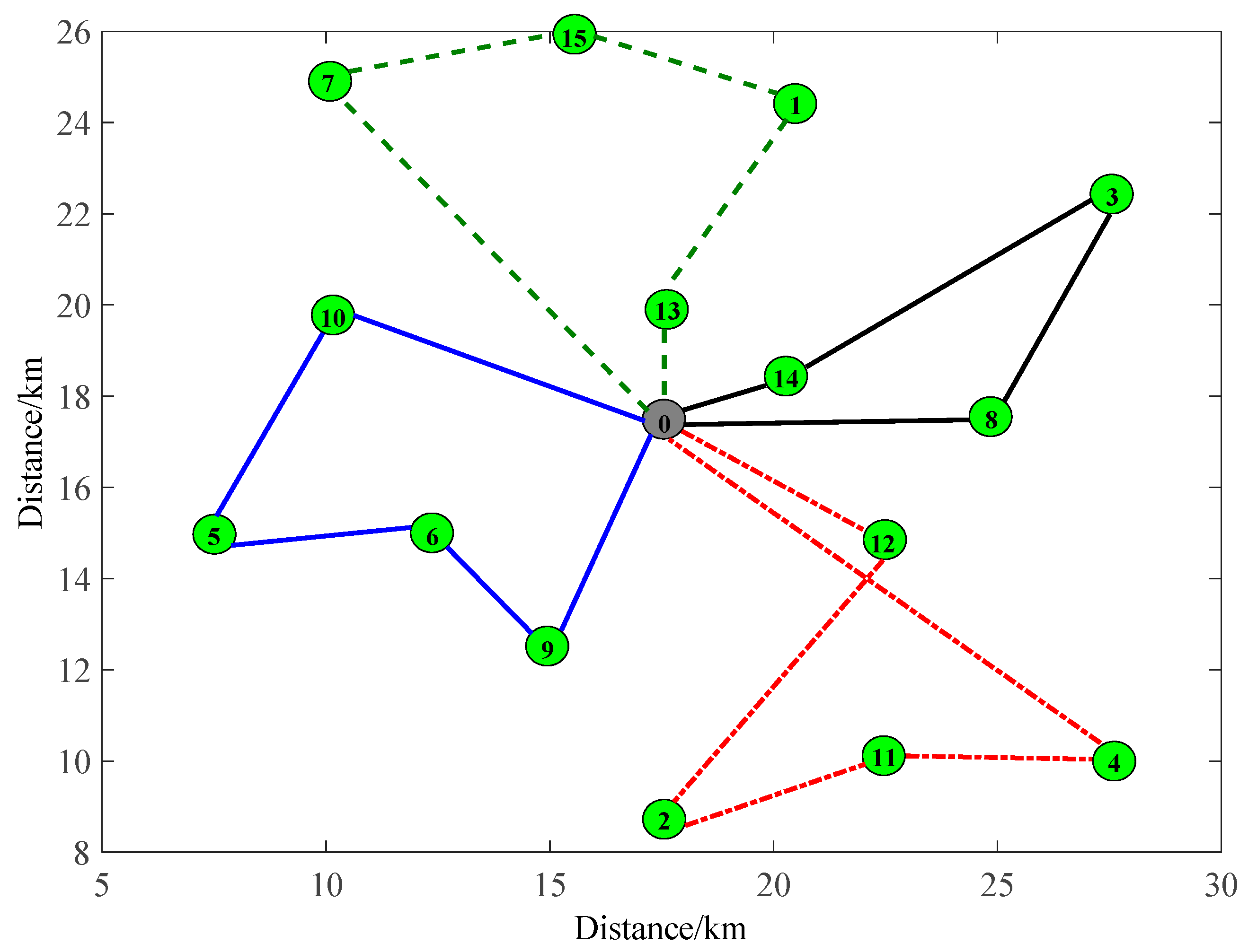
In this case, the logistics network includes a vegetable farm (which is viewed as the distribution center) and 15 consumers . The consumer locations and online order demands, as well as the time windows of consumer orders, are all known.
The distribution center has two kinds of vegetables, and , , [ (simplified as ), , , , and . The GAAO parameters are set as follows: , , , and . Figure 3 shows the spatial coordinate of each consumer (cited by Solomon’s problem [40]). Table 1 gives the consumer information.
We test the basic numerical experiments 20 times, and the optimal results of GAAO are shown in Table 2 and Figure 4. Four vehicles are provided in this distribution service, and the objective value is 2687.3 CNY. The iteration time of GAAO is 186.3 s. The consumer with an earlier time window has a service priority, which indicates that optimal routes are not according to the shortest paths but are selected by the time window constraints in the model.
5.2. Sensitivity Analyses on Postharvest Quality Deterioration Factors
In order to research the relationship between the postharvest quality deterioration factor and the objective value, we vary and from 0.1 to 0.9, respectively. As shown in Figure 5a, the objective value increases as the postharvest quality deterioration factors increase. Figure 5b demonstrates the magnitude of variation in objective value with . In the case of and both being small, due to the slow decay of vegetables, the farm managers have more time to fulfill orders, which makes little gaps between the objective values. In other words, the farm managers can ignore the postharvest quality deterioration cost and select the optimal route with the minimum distribution cost. In the case where and are both large, there is a significant jump in the objective value, since the time sensitivity of the vegetables increases substantially. That is to say, the farm managers need to arrange more vehicles in this case to fulfill the vegetable distribution in a shorter time, which leads to higher costs inevitably.
In general, we can draw two managerial insights. On one hand, controlling the postharvest quality deterioration factor of vegetables is an effective method to reduce the total cost, such as cold-chain transportation or food preservation techniques. On the other hand, when the perishability of vegetable is high, the farm managers could shorten the distribution time by increasing the vehicle number to satisfy the fresh quality requirement of consumers.
5.3. Medium to Large-Scale Numerical Experiments and Comparisons Result between GA and GAAO
In this section, we use 10 different medium–large scale numerical experiments to demonstrate the advantage and efficiency of GAAO. The number of consumers increases from 20 to 110.
We report the computational results of GA and GAAO, and compare the time gap and iteration gap in Table 3. The maximum iteration number of GAAO is 432, while the minimum iteration number of GA is 425. The iteration number of GAAO is significantly less than that of GA, which indicates that GAAO is more efficient. We draw a conclusion that GAAO is superior to GA because GAAO saves at least 10% CPU time and has at least a 20% iteration gap. In other words, compared with GA, GAAO can reduce the iteration and converge the optimal solution in a shorter amount of time.
Figure 6a shows that the trend of GAAO iterations changes from 100 to 300 gradually with the increasing experiment scales, and that of GA iterations ranges from 420 to 900. From Case 1 to Case 6, the iteration gaps between GAAO and GA are all above 50%, but in Case 7 to Case 10, the iteration gaps are smaller. This difference indicates that the GAAO has a distinct solution advantage when the consumer number is less than 70. Figure 6b demonstrates the comparison of CPU time between GAAO and GA. In these cases, GAAO is superior to GA significantly in CPU time. Generally, the performance of GAAO proposed in this paper is consistently better than that of GA in solving the integrated optimization of harvest and farm-to-door distribution, and could obtain an optimal solution more quickly.
6. Conclusions
In this paper, we propose an integrated optimization model that simultaneously considers vegetable harvest and farm-to-door distribution. To capture the perishable feature of vegetables, we formulate a quadratic postharvest quality deterioration function. The optimization model integrates the decisions regarding the harvest time, delivery vehicle assignment, and farm-to-door distribution planning in terms of consumers’ demand requirements and time windows. Moreover, we design a GAAO to solve the proposed model. Finally, numerical results are reported to show the efficiency and effectiveness of the proposed model and solution algorithm, and managerial insights are offered for vegetable online retailing in practice. The numerical results show that the GAAO can obtain the optimal solution with an average 24% CPU time and an iteration number that is 48% less than that of GA. Generally, compared with the traditional vegetable supply chain, our study suggests that integrating harvest and farm-to-door distribution scheduling can reduce the postharvest quality deterioration of vegetables and subsequent distribution costs dramatically.
Our work serves as an initial effort on integrated harvest and farm-to-door distribution scheduling for vegetable online retailing. Several promising directions for future research remain. Firstly, all order information for a certain period in this model is assumed to be determined. In practice, the consumer orders arrive randomly, and such information could be forecasted in advance, which will lead to a scenario-based stochastic programming model. Secondly, we only consider common heterogeneous vehicles in this paper. Considering different types of refrigerated vehicles with variable capacity and multiple compartments for perishable products is also a future research direction. Finally, our model sets most factors to certainty. Incorporating some uncertain factors into harvest and distribution scheduling is an important future research direction, such as the uncertainty of temperature or road conditions.
Author Contributions
Y.J. conceived and designed the research work; Y.J. and B.B. wrote the paper together. L.L. checked the expression in English.
Funding
This research has been supported by the National Natural Science Foundation of China [71803084], Humanity and Social Science Youth Foundation of Ministry of Education of China [17YJC630048], Natural Science Foundation of Jiangsu Province [BK20160742], Fundamental Research Funds for the Central Universities [NAU: SKYC2017007; NAU: SKYZ2017025; NAU: KJQN201960; NAU: KYZ201663], and Project of Philosophy and Social Science Research in Colleges and Universities in Jiangsu [2017SJB0030].
Conflicts of Interest
The authors declare no conflict of interest.
References
- China Industry Information. Available online: http://www.chyxx.com/industry/201808/666953 (accessed on 14 August 2018).
- Kang, C.; Moon, J.; Kim, T.; Choe, Y. Why consumers go to online grocery: Comparing vegetables with grains. In Proceedings of the 49th Hawaii International Conference on System Sciences (HICSS), Koloa, HI, USA, 5–8 January 2016; pp. 3604–3613. [Google Scholar]
- Li, Y.; Sun, Y.; Zhang, Y.; Hu, X. Online grocery retailing for fresh products with order cancellation and refund options. J. Supply Chain Oper. Manag. 2018, 16, 1–16. [Google Scholar]
- Smith, D.; Sparks, L. Temperature controlled supply chains. In Food Supply Chain Management; Bourlakis, M.A., Weightman, P.W.H., Eds.; Blackwell Press: Oxford, UK, 2004; Volume 12, pp. 179–198. [Google Scholar]
- Bustos, C.A.; Moors, E.H.M. Reducing post-harvest food losses through innovative collaboration: Insights from the Colombian and Mexican avocado supply chains. J. Clean. Prod. 2018, 199, 1020–1034. [Google Scholar] [CrossRef] [Green Version]
- Pavlista, A.D.; Santra, D.K. Planting and harvest dates, and irrigation on fenugreek in the semi-arid high plains of the USA. Ind. Crop. Prod. 2016, 94, 65–71. [Google Scholar] [CrossRef] [Green Version]
- Thuankaewsing, S.; Khamjan, S.; Piewthongngam, K.; Pathumnakul, S. Harvest scheduling algorithm to equalize supplier benefits: A case study from the Thai sugar cane industry. Comput. Electron. Agric. 2015, 110, 42–55. [Google Scholar] [CrossRef]
- Lamsal, K.; Jones, P.C.; Thomas, B.W. Continuous time scheduling for sugarcane harvest logistics in Louisiana. Int. J. Prod. Res. 2016, 54, 616–627. [Google Scholar] [CrossRef]
- Soto-Silva, W.E.; González-Araya, M.C.; Oliva-Fernández, M.A.; Plà-Aragonés, L.M. Optimizing fresh food logistics for processing: Application for a large Chilean apple supply chain. Comput. Electron. Agric. 2017, 136, 42–57. [Google Scholar] [CrossRef]
- Devapriya, P.; Ferrell, W.; Geismar, N. Integrated production and distribution scheduling with a perishable product. Eur. J. Oper. Res. 2017, 259, 906–916. [Google Scholar] [CrossRef]
- Reis, S.A.; Leal, J.E. A deterministic mathematical model to support temporal and spatial decisions of the soybean supply chain. J. Transp. Geogr. 2015, 43, 48–58. [Google Scholar] [CrossRef]
- Ghare, P.M. A model for an exponentially decaying inventory. J. Ind. Engng. 1963, 14, 238–243. [Google Scholar]
- Piramuthu, S.; Zhou, W. RFID and perishable inventory management with shelf-space and freshness dependent demand. Int. J. Prod. Econ. 2013, 144, 635–640. [Google Scholar] [CrossRef]
- Rahdar, M.; Nookabadi, A.S. Coordination mechanism for a deteriorating item in a two-level supply chain system. Appl. Math. Model. 2014, 38, 2884–2900. [Google Scholar] [CrossRef]
- Rong, A.; Akkerman, R.; Grunow, M. An optimization approach for managing fresh food quality throughout the supply chain. Int. J. Prod. Econ. 2011, 131, 421–429. [Google Scholar] [CrossRef]
- Wang, X.; Li, D. A dynamic product quality evaluation based pricing model for perishable food supply chains. Omega 2012, 40, 906–917. [Google Scholar] [CrossRef]
- Mohapatra, P.; Roy, S. Mathematical Model for Optimization of Perishable Resources with Uniform Decay. In Computational Intelligence in Data Mining; Springer: Berlin/Heidelberg, Germany, 2016; Volume 2, pp. 447–454. [Google Scholar]
- De Keizer, M.; Akkerman, R.; Grunow, M.; Bloemhof, J.M.; Haijema, R.; van der Vorst, J.G. Logistics network design for perishable products with heterogeneous quality decay. Eur. J. Oper. Res. 2017, 262, 535–549. [Google Scholar] [CrossRef]
- Ferrer, J.C.; Mac Cawley, A.; Maturana, S.; Toloza, S.; Vera, J. An optimization approach for scheduling wine grape harvest operations. Int. J. Prod. Econ. 2008, 112, 985–999. [Google Scholar] [CrossRef]
- Herbon, A.; Levner, E.; Cheng, T.C.E. Perishable inventory management with dynamic pricing using time–temperature indicators linked to automatic detecting devices. Int. J. Prod. Econ. 2014, 147, 605–613. [Google Scholar] [CrossRef]
- Cai, X.; Chen, J.; Xiao, Y.; Xu, X. Optimization and coordination of fresh product supply chains with freshness-keeping effort. Prod. Oper. Manag. 2010, 19, 261–278. [Google Scholar] [CrossRef]
- Díaz-Pérez, M.; Carreño-Ortega, Á.; Salinas-Andújar, J.A.; Callejón-Ferre, Á.J. Logistic Regression to Evaluate the Marketability of Pepper Cultivars. Agronomy 2019, 9, 125. [Google Scholar] [CrossRef]
- Nekvapil, F.; Brezestean, I.; Barchewitz, D.; Glamuzina, B.; Chiş, V.; Pinzaru, S.C. Citrus fruits freshness assessment using Raman spectroscopy. Food Chem. 2018, 242, 560–567. [Google Scholar] [CrossRef]
- Amorim, P.; Günther, H.O.; Almada-Lobo, B. Multi-objective integrated production and distribution planning of perishable products. Int. J. Prod. Econ. 2012, 138, 89–101. [Google Scholar] [CrossRef]
- Wang, X.; Wang, M.; Ruan, J.; Zhan, H. The multi-objective optimization for perishable food distribution route considering temporal-spatial distance. Procedia Comput. Sci. 2016, 96, 1211–1220. [Google Scholar] [CrossRef]
- Arnaout, J.P.M.; Maatouk, M. Optimization of quality and operational costs through improved scheduling of harvest operations. Int. Trans. Oper. Res. 2010, 17, 595–605. [Google Scholar] [CrossRef]
- González-Araya, M.C.; Soto-Silva, W.E.; Espejo, L.G.A. Harvest Planning in Apple Orchards Using an Optimization Model. In Handbook of Operations Research in Agriculture and the Agri-Food Industry; Springer: New York, NY, USA, 2015; pp. 79–105. [Google Scholar]
- An, K.; Ouyang, Y. Robust grain supply chain design considering post-harvest loss and harvest timing equilibrium. Transp. Res. Part E Logist. Transp. Rev. 2016, 88, 110–128. [Google Scholar] [CrossRef] [Green Version]
- Ferreira, M.D.; Sanchez, A.C.; Braunbeck, O.A.; Santos, E.A. Harvesting fruits using a mobile platform: A case study applied to citrus. Eng. Agr. 2018, 38, 293–299. [Google Scholar] [CrossRef]
- Takeda, F.; Yang, W.; Li, C.; Freivalds, A.; Sung, K.; Xu, R.; Hu, B.; Williamson, J.; Sargent, S. Applying new technologies to transform blueberry harvesting. Agronomy 2017, 7, 33. [Google Scholar] [CrossRef]
- Ceccarelli, A.; Farneti, B.; Frisina, C.; Allen, D.; Donati, I.; Cellini, A.; Costa, G.; Spinelli, F.; Stefanelli, D. Harvest maturity stage and cold storage length influence on flavour development in peach fruit. Agronomy 2019, 9, 10. [Google Scholar] [CrossRef]
- Ahumada, O.; Villalobos, J.R. Operational model for planning the harvest and distribution of perishable agricultural products. Int. J. Prod. Econ. 2011, 133, 677–687. [Google Scholar] [CrossRef]
- Amorim, P.; Almada-Lobo, B. The impact of food perishability issues in the vehicle routing problem. Comput. Ind. Eng. 2014, 67, 223–233. [Google Scholar] [CrossRef]
- Moons, S.; Ramaekers, K.; Caris, A.; Ardae, Y. Integrating production scheduling and vehicle routing decisions at the operational decision level: A review and discussion. Comput. Ind. Eng. 2017, 104, 224–245. [Google Scholar] [CrossRef]
- Hsiao, Y.H.; Chen, M.C.; Chin, C.L. Distribution planning for perishable foods in cold chains with quality concerns: Formulation and solution procedure. Trends Food Sci. Technol. 2017, 61, 80–93. [Google Scholar] [CrossRef]
- Ahumada, O.; Villalobos, J.R.; Mason, A.N. Tactical planning of the production and distribution of fresh agricultural products under uncertainty. Agric. Syst. 2012, 112, 17–26. [Google Scholar] [CrossRef]
- Farahani, P.; Grunow, M.; Günther, H.O. Integrated production and distribution planning for perishable food products. Flex. Serv. Manuf. J. 2012, 24, 28–51. [Google Scholar] [CrossRef]
- Jing, Y.; Li, W. Integrated recycling-integrated production-distribution planning for decentralized closed-loop supply chain. J. Ind. Manag. Optim. 2018, 14, 511–539. [Google Scholar] [CrossRef]
- Savelsbergh, M.W.P. Local search for routing problem with time windows. Ann. Oper. Res. 1985, 35, 254–265. [Google Scholar] [CrossRef]
- Solomon, M.M. Algorithms for the vehicle routing and scheduling problems with time window constraints. Oper. Res. 1987, 35, 254–265. [Google Scholar] [CrossRef]
Figure 1.
Diagram for harvest and farm-to-door distribution scheduling for vegetable online retailing.
Figure 1.
Diagram for harvest and farm-to-door distribution scheduling for vegetable online retailing.
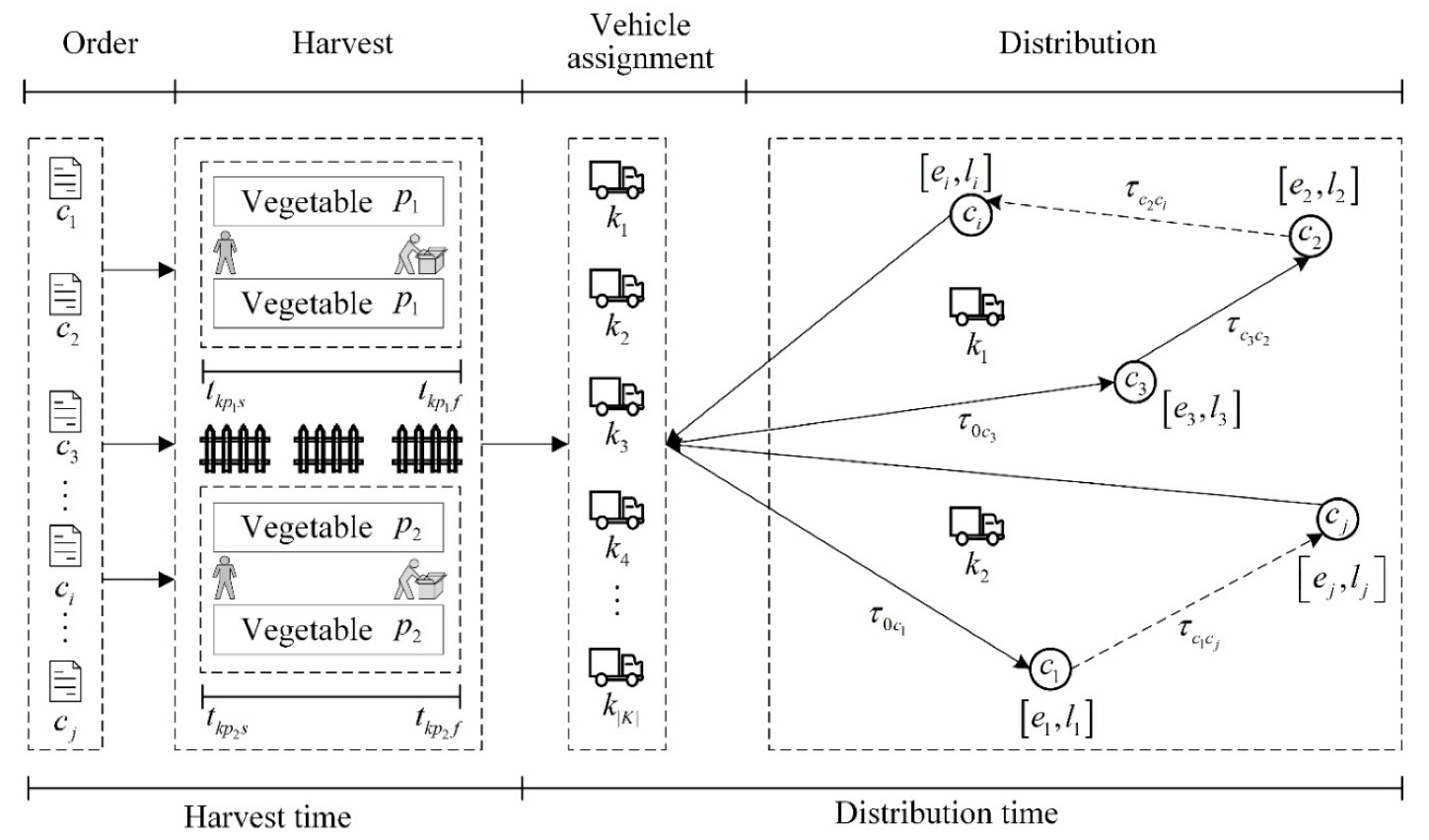
Figure 2.
Flow chart of genetic algorithm with adaptive operators (GAAO).

Figure 3.
Schematic diagram of spatial coordinates.

Figure 4.
The optimal vehicle routing.

Figure 5.
Relationship between objective value and postharvest quality deterioration factor. (a) Objective value under different values of and ; (b) The variation trend between objective value and .
Figure 5.
Relationship between objective value and postharvest quality deterioration factor. (a) Objective value under different values of and ; (b) The variation trend between objective value and .

Figure 6.
Comparison of computational performance between GA (genetic algorithm) and GAAO (genetic algorithm with adaptive operators). (a) Comparison of iteration between GA and GAAO; (b) Comparison of CPU time between GA and GAAO.
Figure 6.
Comparison of computational performance between GA (genetic algorithm) and GAAO (genetic algorithm with adaptive operators). (a) Comparison of iteration between GA and GAAO; (b) Comparison of CPU time between GA and GAAO.


Table 1.
The consumer information.
| Consumer Number | Coordinate (km) | Demand (kg) | Time Window | Consumer Number | Coordinate (km) | Demand (kg) | Time Window |
|---|---|---|---|---|---|---|---|
| 1 | (20.5, 24.5) | (15, 23) | [13:30, 16:00] | 9 | (15, 12.5) | (11, 19) | [13:30, 15:50] |
| 2 | (17.5, 8.5) | (18, 14) | [13:50, 15:55] | 10 | (10, 20) | (13, 28) | [11:40, 15:00] |
| 3 | (27.5, 22.5) | (30, 20) | [14:10, 17:00] | 11 | (22.5, 10) | (7, 25) | [12:35, 14:50] |
| 4 | (27.5, 10) | (19, 16) | [10:40, 14:00] | 12 | (22.5, 15) | (12, 15) | [13:40, 15:10] |
| 5 | (7.5, 15) | (15, 26) | [12:10, 15:00] | 13 | (17.5, 20) | (19, 17) | [14:10, 16:35] |
| 6 | (12.5, 15) | (20, 24) | [11:10, 16:20] | 14 | (20.5, 18.5) | (10, 12) | [12:40, 14:40] |
| 7 | (10, 25) | (10, 23) | [12:00, 15:10] | 15 | (15.5, 26) | (14, 22) | [11:50, 13:00] |
| 8 | (25, 17.5) | (25, 16) | [12:00, 17:00] |
Table 2.
Optimal results of GAAO.
| Number | The Optimal Vehicle Routing | ||
|---|---|---|---|
| Vehicle 1 | 0→8→3→14→0 | ||
| Vehicle 2 | 0→10→5→6→9→0 | ||
| Vehicle 3 | 0→7→15→1→13→0 | ||
| Vehicle 4 | 0→12→2→11→14→0 | ||
| Experimental Results | Objective value (CNY) | Number of Vehicles | Iteration Time/s |
| 2687.3 | 4 | 186.3 | |
Table 3.
Numerical results of medium to large-scale cases.
| Case | Variable Sizes | GA | GAAO | Time Gap (%) | Iteration Gap (%) | |||
|---|---|---|---|---|---|---|---|---|
| Con. | Products | CPU Time/s | Iteration | CPU Time/s | Iteration | |||
| 1 | 20 | 2 | 363 | 426 | 191 | 104 | 47.38 | 75.52 |
| 2 | 30 | 2 | 366 | 432 | 243 | 174 | 33.61 | 59.87 |
| 3 | 40 | 2 | 398 | 494 | 289 | 197 | 27.39 | 60.05 |
| 4 | 50 | 2 | 408 | 504 | 347 | 228 | 14.95 | 54.78 |
| 5 | 60 | 2 | 411 | 903 | 368 | 264 | 10.46 | 70.74 |
| 6 | 70 | 2 | 467 | 652 | 389 | 271 | 16.70 | 58.41 |
| 7 | 80 | 2 | 491 | 541 | 401 | 337 | 18.33 | 37.79 |
| 8 | 90 | 2 | 528 | 425 | 423 | 366 | 19.89 | 13.91 |
| 9 | 100 | 2 | 610 | 481 | 456 | 371 | 25.25 | 22.89 |
| 10 | 110 | 2 | 723 | 621 | 516 | 432 | 28.63 | 30.36 |
GA: genetic algorithm. Con.: consumer number. . .
© 2019 by the authors. Licensee MDPI, Basel, Switzerland. This article is an open access article distributed under the terms and conditions of the Creative Commons Attribution (CC BY) license (http://creativecommons.org/licenses/by/4.0/).
Share and Cite
MDPI and ACS Style
Jiang, Y.; Bian, B.; Li, L. Integrated Harvest and Farm-to-Door Distribution Scheduling with Postharvest Quality Deterioration for Vegetable Online Retailing. Agronomy 2019, 9, 724. https://doi.org/10.3390/agronomy9110724
AMA Style
Jiang Y, Bian B, Li L. Integrated Harvest and Farm-to-Door Distribution Scheduling with Postharvest Quality Deterioration for Vegetable Online Retailing. Agronomy. 2019; 9(11):724. https://doi.org/10.3390/agronomy9110724
Chicago/Turabian StyleJiang, Yiping, Bei Bian, and Lingling Li. 2019. "Integrated Harvest and Farm-to-Door Distribution Scheduling with Postharvest Quality Deterioration for Vegetable Online Retailing" Agronomy 9, no. 11: 724. https://doi.org/10.3390/agronomy9110724
Note that from the first issue of 2016, this journal uses article numbers instead of page numbers. See further details here.