Evaluation of Evapotranspiration from Eddy Covariance Using Large Weighing Lysimeters

Abstract

Evapotranspiration (ET) is an important component in the water budget and used extensively in water resources management such as water planning and irrigation scheduling. In semi-arid regions, irrigation is used to supplement limited and erratic growing season rainfall to meet crop water demand. Although lysimetery is considered the most accurate method for crop water use measurements, high-precision weighing lysimeters are expensive to build and operate. Alternatively, other measurement systems such as eddy covariance (EC) are being used to estimate crop water use. However, due to numerous explicit and implicit assumptions in the EC method, an energy balance closure problem is widely acknowledged. In this study, three EC systems were installed in a field containing a large weighing lysimeter at heights of 2.5, 4.5, and 8.5 m. Sensible heat flux (H) and ET from each EC system were evaluated against the lysimeter. Energy balance closure ranged from 64% to 67% for the three sensor heights. Results showed that all three EC systems underestimated H and consequently overestimated ET; however, the underestimation of H was greater in magnitude than the overestimation of ET. Analysis showed accuracy of ET was greater than energy balance closure with error rates of 20%–30% for half-hourly values. Further analysis of error rates throughout the growing season showed that energy balance closure and ET accuracy were greatest early in the season and larger error was found after plants reached their maximum height. Therefore, large errors associated with increased biomass may indicate unaccounted-for energy stored in the plant canopy as one source of error. Summing the half-hourly data to a daily time-step drastically reduced error in ET to 10%–15%, indicating that EC has potential for use in agricultural water management.

1. Introduction

Fresh water is an essential resource that is becoming increasingly limited. In some arid and semi-arid regions, groundwater resources are being exhausted, with little to no surface water available as an alternate source. Proper water resources management is essential for these areas to extend the availability of water resources. In many cases, water management strategies rely on the use of evapotranspiration (ET) to account for some of the water losses. ET is a combined term that represents water lost through evaporation from the soil or plant surface, as well as water lost through transpiration from the plant. In many regions, such as the Texas High Plains (THP), ET is the largest water loss component in the hydrologic budget [1]. This fact makes accurate ET estimates vital for accurately and properly managing crop water. In the THP, and the remainder of the Southern Ogallala Aquifer region, groundwater recharge is very low at ~11 mm yr⁻¹ [2]. With such low recharge, the Ogallala Aquifer is deemed a finite resource. To preserve this natural resource for future generations, conserving the remaining water is paramount.

The THP lies in the Southern Great Plains near the southern end of the Ogallala Aquifer (Figure 1). Agriculture is the predominant land use and irrigated land accounts for the majority of the agricultural production in this region. In the state of Texas, irrigation accounts for 60% of total water use; however, in the THP, irrigation accounts for 89% of the total water use [1]. The THP is a major corn-, cotton-, wheat-, and sorghum-producing region, with much of the agricultural production under irrigation. The vast majority of irrigation water is withdrawn from the Ogallala Aquifer. With limited and sporadic rainfall, the Ogallala Aquifer receives little to no recharge in this region, and is essentially being mined; therefore, conservation is an integral part of the regional water plan [3]. The northern and southern parts of the THP are similar in size; however, 1.1 million ha are irrigated in the northern THP, while over 760,000 ha are irrigated in the southern THP [4]. In both regions average irrigated crop yields are at least double that of dryland yields.

Conservation strategies such as effective irrigation scheduling, in addition to water availability modeling, rely on ET estimates, with greater accuracy leading to greater efficacy. Many instruments and methods are available for estimating ET, from simple equations using only one or two meteorological parameters to very complex sensor systems or models. Lysimetery is considered the standard for ET measurement [5], but lysimeters are typically labor- and cost-prohibitive. Eddy covariance (EC) is a portable and manageable system for estimating ET. EC systems have predominantly been used for meteorological and research purposes; however, their popularity and availability has led to their use in agricultural and water resources research.

EC systems are based on the theory that, as wind moves, it does not move unidirectionally but in three-dimensional circular patterns [6]. In addition, as the air moves, it carries molecules of water vapor and other gases such as carbon dioxide and methane. If the speed of these eddies can be measured in all three directions, the net exchange of these molecules between the surface and the atmosphere can be determined. In conjunction, a gas analyzer can be used to measure the amounts of water vapor (or other gases) the air contains at that moment. The covariance between the movement of the air mass and the composition of that same air mass can be used to determine the heat and water flux (or fluxes of carbon dioxide and methane), which can be used to calculate the sensible heat flux (H), latent heat flux (LE), and ET. This is the basis for EC systems, where a three-dimensional sonic anemometer and an infrared gas analyzer (or krypton hygrometer) are used to collect the aforementioned data at a high frequency. With H and LE derived from EC fluxes, the net radiation (R_n) and soil heat flux (G) can be measured to obtain the four energy balance (EB) components. Assessing the EB closure is one metric of evaluating the accuracy of the H and LE measurements from EC. A widely acknowledged issue with EC is the lack of energy balance closure. Based on the laws of thermodynamics, the R_n should be partitioned into the other three energy balance components yielding a zero sum:

$$R_n-LE-H-G=0$$

(1)

When using H and LE from EC measurements, these energy components do not converge, especially for heterogeneous land-surface (canopy) conditions. This type of imbalance of energy components along with main components of H and LE, is not explicitly known. Even with the widely acknowledged EB closure issue [7], EC has been used extensively for various applications all over the world. The use of EC has increased in agricultural research for crop coefficient development [8,9], remote sensing analysis [10,11], carbon sequestration [12], and perhaps atmosphere‒land surface interaction processing. Although the EB closure aspect has been investigated, the effects on the accuracy of ET have not been thoroughly evaluated.

Typical EB closure errors of approximately 20%–30% are widely reported in the literature [13]. In the past, measurement errors for R_n and G were commonly pinpointed as the cause for the closure problem; however, modern sensors are considered much more reliable and accurate [14]. Other reasons for the errors include different scales between the energy balance components, the energy storage in the soil and canopy, and the heterogeneity of the land surface.

In addition to the physiological sources of errors, instrument limitations [15] and data processing can impact flux accuracy and EB closure. Irmak et al. [16] showed residual energy from EC can be affected by the growing season and frictional wind speed based on data collected over a maize (Zea mays L.) field in Nebraska. Higgins [17] showed that the variation in residual energy could be attributed to energy stored in the soil and underestimation of soil heat flux and underestimation of H and LE did not contribute to the residual energy based on data from salt flats in Utah. However, Rannik et al. [18] showed that EC fluxes can contain 10%–30% random error based on theoretical calculations and field measurements.

Based on the available literature, it is evident that EC systems commonly have EB closure errors, indicating that errors exist in both the H and LE measurements. Due to the complexity of determining H and LE values, few studies quantify the error of the fluxes against actual measurements. Lysimeters provide the most accurate ET validation data. The highly accurate ET measurements from a well-designed and operated lysimeter can also be used to derive the turbulent fluxes of H and LE, which should have a high degree of accuracy. However, few studies have evaluated EC systems compared to lysimeters for flux and ET accuracy. Therefore, the objective of this study was to evaluate EC as compared to a lysimeter for accuracy in determining H and ET values in addition to investigating the source of any potential errors.

2. Materials and Methods

2.1. Study Area

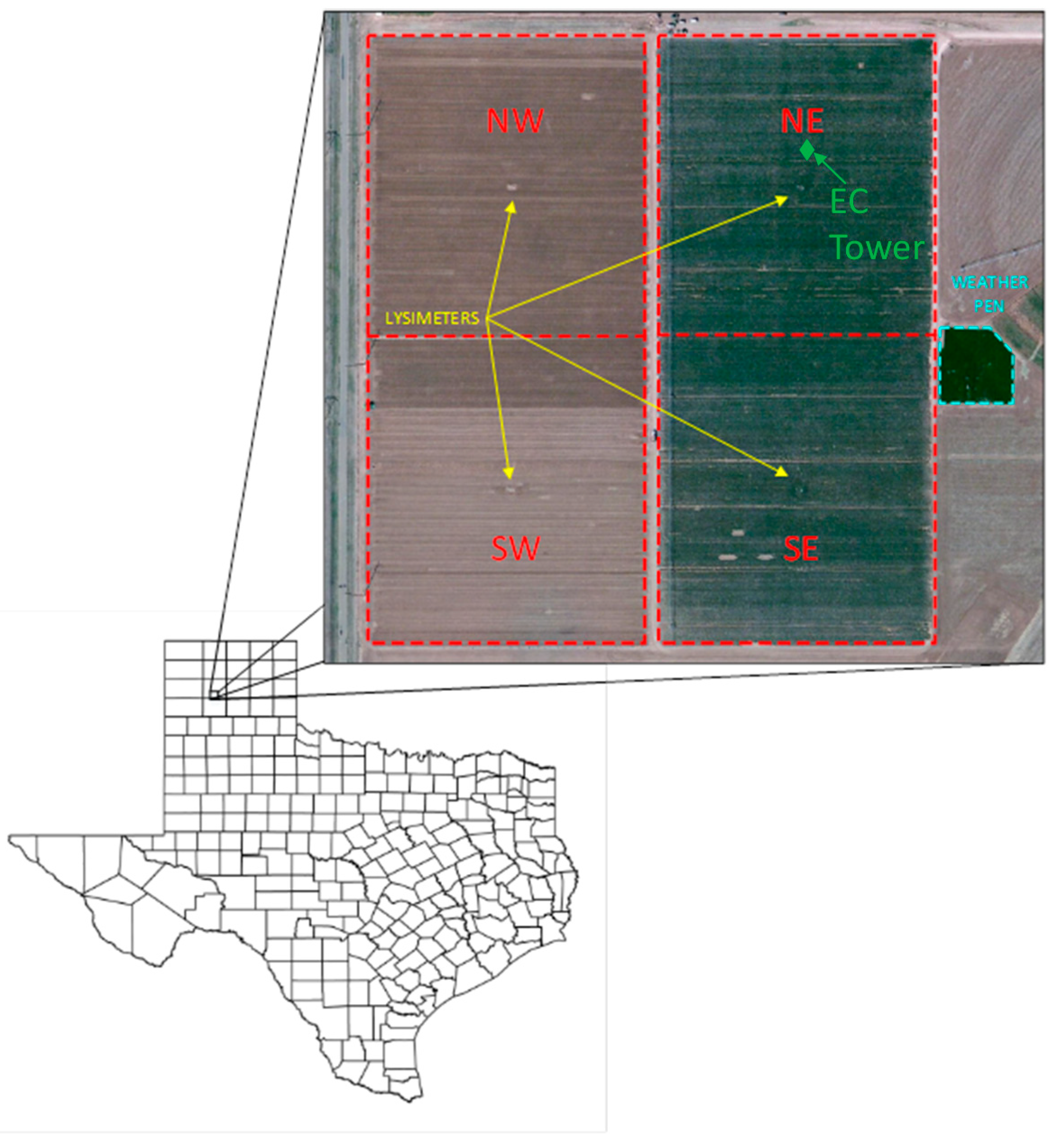
The study area was the USDA-ARS-Conservation and Production Research Laboratory (CPRL), located 17 km west of Amarillo, TX (35.188 N, 102.095 W). The region is classified as semi-arid with approximately 450 mm average annual precipitation. The study site is located inside a 19-ha square field, which is split into four 4.7-ha quadrants (see Figure 2). Each quadrant is roughly 200 by 220 m and contains a large weighing lysimeter located in the center of the field. The east half of the field is irrigated with a subsurface drip and the west half is irrigated using a lateral move sprinkler irrigation system. The northeast (NE) quadrant was used for this study as it provides the greatest fetch with respect to the predominant wind direction (SSW). The field was planted with grain sorghum at a rate of 210,000 seeds per ha (85,000 seeds per acre), which was fully irrigated using subsurface drip at a 23 cm (9 in.) depth and 150 cm (59 in.) lateral spacing.

2.2. Lysimeters

The large weighing lysimeter measures 3 m by 3 m on the surface by 2.3 m deep over a fine sand drainage base. It contains an undisturbed monolithic Pullman clay loam soil profile with subsurface drip irrigation at 23 cm depth. The soil container rests on a large agronomic scale equipped with a counterbalance and load cell system. Initial design and installation details of the lysimeter are provided by [19] and [20]. The lysimeter was later equipped with drainage effluent tanks suspended from the lysimeter by load cells for separate measurement of drainage mass without changing total lysimeter mass. Load cell output is measured and recorded by a precision datalogger. Load cell voltage outputs are converted to mass using calibration equations, and five-minute means are used to develop a base dataset for subsequent processing [21]. Lysimeter mass in kg is converted to a mass-equivalent relative lysimeter storage value (mm of water) by dividing it by the relevant surface area of the lysimeter (~9 m²) and the density of water (1000 kg m³). Equivalent mass values allow for changes in lysimeter mass to be expressed in terms of water flux, defined as mm of water lost or gained per unit time. The lysimeter datalogger mass resolution is better than 0.001 mm when converted to equivalent depth of water. Lysimeter accuracy is, however, determined by the root mean square error (RMSE) of calibration, which has ranged from 0.05 mm to 0.01 mm [5,21]. Lysimeter quality assurance and quality control (QA/QC) and data processing techniques were provided by [22].

Calculating ET in units of equivalent depth of water requires that the change in lysimeter mass be divided by the effective evaporating and transpiring area of the lysimeter [23]. Evett et al. [5] reported that the Bushland lysimeter inside surface area was 8.95 m². However, the area of contribution from captured precipitation or irrigation, as well as ET, extends beyond the lysimeter container resulting in an effective area larger than the physical area of the lysimeter. Evett et al. [5] reported the outside lysimeter surface area was 9.35 m². In this case, a correction factor of 1.05 (9.35 m²/8.95 m²) was applied to ET measurements from the lysimeter.

The lysimeter was designed to be representative of the surrounding field so that measured lysimeter ET closely mimics field ET. Experienced support scientists and technicians are responsible for maintaining lysimeter representativeness as compared to surrounding fields. Careful attention is given to agronomic operations including planting, harvesting, tillage, fertilization, irrigation, and pesticide application such that there should be no distinguishable differences, particularly in height, between the crop grown on the lysimeter and that grown in the surrounding field. To confirm this, multiple neutron probe access sites were located both throughout the field and in the lysimeter to monitor the soil profile water content. Weekly soil water content (SWC) readings from the neutron probes throughout the field are compared to SWC readings from the lysimeter to determine representativeness. In addition to SWC readings, plant mapping and stand counts were periodically taken to ensure the crop growth on the lysimeter approximates the surrounding field. The lysimeter box contains a ~50 mm freeboard lip that extends above the soil surface to limit runoff or run-on to the lysimeter. Similarly, furrow dikes are used to limit runoff and run-on for the surrounding field.

In some instances, field operations prohibited measurements with the lysimeter. For example, maintenance on the lysimeter, or instruments mounted near the lysimeter, would require personnel to step onto the lysimeter box, temporarily increasing the mass. Other operations include draining the percolation storage tanks, which causes an overall decrease in the mass, irrigation applications, and taking neutron probe soil moisture readings. The amount of water drained is measured, but data recorded during the process of draining the tanks are not usable. For sub-daily data, periods of precipitation will reduce data availability since the precipitation cannot be accounted for in the ET for short periods, such as hourly or 30-min intervals. In the instance where operations prohibited data collection, the data from those time intervals were omitted. In the instances where lysimeter data were omitted, the corresponding EC data were also excluded.

2.3. Eddy Covariance System

In this study, three EC systems were installed within an experimental field containing a large weighing lysimeter, planted with grain sorghum, located at the CPRL. The EC systems were installed at 2.5, 4.5, and 8.5 m heights (labeled 2 m, 4 m, 8 m for simplicity) approximately 40 m to the north of the lysimeter and facing due south. The distance between the EC systems and the lysimeter should provide an arrangement where the lysimeter is in the area where the EC systems obtain the greatest contribution to the flux measurements. The NE lysimeter field quadrant (Figure 2) was chosen to provide the maximum amount of fetch so that the EC footprint would contain a highly homogenous surface.

The EC systems consisted of a three-dimensional sonic anemometer (CSAT3, Campbell Scientific, Logan, UT, USA) and an open path infrared gas analyzer (LI-7500A, LI-COR Biosciences, Lincoln, NE, USA). Additional instruments installed near the lysimeter included an air temperature and relative humidity sensor (HMP155, Vaisala, Helsinki, Finland), six soil heat flux plates (HFT-3, Radiation Energy Balance Systems, Bellevue, WA, USA), four soil moisture sensors (Acclima 315, Acclima Inc., Meridian, ID, USA), an infrared thermometer (IRT), and a net radiometer (Q*7.1, Radiation Energy Balance Systems). The additional meteorological instruments were mounted three meters above the soil surface on a mast at the edge of the lysimeter container. The instruments were connected to a datalogger (CR6, Campbell Scientific) with measurements taken at 6-s intervals, which were then summed or averaged to 30-min data. The additional sensors installed near the lysimeter underwent QA/QC analysis according to [24], performed on each 30-min period. QA/QC for the R_n involved comparing measured R_n with the sum of measured downwelling and upwelling short- and longwave radiation from a pyranometer (CM14, Kipp & Zonen, Delft, The Netherlands) and a pyrgeometer (CG4, Kipp & Zonen). The pyranometer and pyrgeometer were also mounted at three meters on the same mast as the net radiometer for the purpose of validating the net radiation measurements. In addition, the solar irradiance component was compared with the calculated theoretical maximum clear sky solar irradiance.

The 20 Hz EC data were processed using standard corrections and adjustments prior to the flux calculations. Processing involved applying coordinate rotations, despiking [25], time lag compensation using cross-correlation maximization, Webb‒Pearman‒Leuning (WPL) corrections [26], and high and low-pass filtering [27] using block averaging. The EC system determines ET from the LE values determined by the water flux. The EC data analysis software EddyPro (LI-COR Inc.) was used to calculate H and LE at 30-min intervals from the 20 Hz measurements. After all standard corrections half-hour H and LE were calculated. The flux for any gas ($F$) can be calculated from the EC data by:

$$F=\overline{\overline{\rho w^{\prime }{s}^{\prime }}}$$

(2)

where $\overline{\rho }$ is the mean air density, and $\overline{w^{\prime }}$ and $\overline{s^{\prime }}$ are deviations from the mean for wind speed and dry mole fraction, respectively [6]. The dry mole fraction can be determined for any gas or variable of interest. From this principle, H and LE can be calculated by:

$$H=\overline{\rho }{C}_p\overline{\overline{w^{\prime }{T}^{\prime }}}$$

(3)

and

$$LE=\lambda \frac{M_w/M_a}{\overline{P}}\overline{\rho w^{\prime }{e}^{\prime }}$$

(4)

Soil water and temperature data were used to calculate G at the soil surface by the calorimetric method, and surface G was used in all EB calculations. The calorimetric method used in this study was described by Colaizzi et al. [28]; briefly, it used the soil water and temperature measurements to calculate the change in soil heat storage between the surface and the depth of the soil heat flux plates in 30-min time steps. The H, LE, and G were subtracted from the R_n to determine the EB residual. EB closure was evaluated using the slope of the regression equation, as well as the RMSE expressed as a percentage (%RMSE) of the available energy (AE = R_n − G). Using the regression slope has been a common method for evaluating EB closure for EC; however, there are studies in the literature that use other methods, such as the energy balance ratio (AE/H + LE) [29]. For this study, the %RMSE was used to provide multiple EB closure values and a comparison with the regression slope. After determining the magnitude of the residual energy, the residual was distributed between H and LE using the Bowen ratio to force the EB to close at each 30-min interval. The corrected H and LE were used for evaluation and to determine ET for the EC system at the 30-min time-step.

2.4. Accuracy Analysis

In addition to evaluating ET, H from EC was compared to H from the lysimeter. H was back calculated from the lysimeter by converting the ET to LE and accounting the residual of the EB to H. Latent heat flux can by calculated from ET by:

$$LE=\frac{ET(mm)\lambda }{time(\sec )}$$

(5)

where λ is the latent heat of vaporization (J kg⁻¹). The latent heat of vaporization can be calculated from the surface temperature, T_s (°C) by:

$$\lambda =\left(2.501-0.0236T_s\right){10}^6$$

(6)

Surface temperature was obtained from the IRT installed on the lysimeter and used to determine the latent heat of vaporization for each 30-min period. Using the lysimeter ET data, the LE was calculated by multiplying the ET by the latent heat of vaporization and dividing by 1800 s to convert to the 30-min period.

During nighttime hours, LE, and subsequently ET, becomes very small. The much smaller values can exhibit much more variation. Even though the magnitude of the differences may be small, relative percentage differences can be large. To determine the effects of including nighttime ET, evaluations were included using only daytime ET data. This analysis should provide an indication as to how much of the overall variation is influenced by the much smaller nighttime values. In addition, since most water management practices and decisions are performed at a daily time-step, the half hourly lysimeter and EC data were summed to evaluate the effects of daily data from EC.

As the crop height increases, the surface roughness and dynamics change, which affects flux calculations. To investigate the effects of the changing surface, analyses were separated into periods corresponding to crop height. Analysis of variance (ANOVA) tests were used to evaluate differences between various periods. Although the ANOVA results do not provide any explanation of differences, it was selected for this study to evaluate the significance of any differences in values for the different periods and comparisons.

For the accuracy analysis, the H and ET from the EC were compared against the lysimeter. Statistics were calculated using SAS version 9.4 (SAS Institute Inc., Cary, NC, USA) where RMSE and the %RMSE were used to evaluate accuracy, in addition to regression analyses to test the EC-lysimeter relationship for linearity and for how well the data fit the 1:1 line. The RMSE provided the magnitude of errors for each analysis and the %RMSE provided relative error. In many cases with ET data using short time intervals, the values can be quite small, making differences appear insignificant. Using relative statistics changes the perspective allowing differences to be more easily detected.

3. Results

The period of data for this study was 28 July 2015 to 29 October 2015. As the sorghum was planted on 23 June 2015, the crop height at the beginning of this study was 0.54 m and reached a maximum height of 1.13 m on 24 August 2015. The crop height throughout the year is presented in

Table 1. Crop height measurements for the 2015 summer growing season.

Date Range	Crop Height
25 July–4 August	0.54 m
5 August–10 August	0.80 m
11 August–16 August	0.91 m
17 August–20 August	1.07 m
21 August–23 August	1.10 m
24 August–29 October	1.13 m

. Installation of the instruments was delayed allowing field operations that would not be possible after the instrument towers were in place. Instrument removal took place October 30, 2015 to allow for harvest, which took place 13 November 2015. The maximum height measurement on 24 August 2015 coincided with the majority of the field reaching the flowering stage and having the maximum leaf area index (LAI) of 4.20 m m⁻¹. After reaching maximum height, the crop reached the soft dough stage on September 14, 2015 (LAI = 3.72), hard dough on 28 September 2015 (LAI = 3.6), and finally reaching black layer on 20 October 2015 (LAI = 3.19).

3.1. Energy Balance Closure

EB closure was 67, 65, and 64% for the 2 m, 4 m, and 8 m EC systems (see Figure 3), respectively, based on the slope of the regression lines. Using the %RMSE as a measure of EB closure resulted in 57, 50, and 51% closure for the 2 m, 4 m, and 8 m systems, respectively. The values from the regression slopes are comparable to those typically found in the literature. Similar closure was found for each of the three sensor heights. ANOVA results showed statistical differences (p < 0.001) between the AE and fluxes for all sensor heights. Closure may have been related to sensor height as the lowest sensor produced the greatest EB closure. It is well known that EC source area increases with sensor height. Flux footprint was determined using the Kljun et al. footprint model [30], as calculated by the EddyPro software for each half-hourly interval. The average contribution distance, which accounted for 70% of flux contribution, was 65.6 m, 189.2 m, and 530.9 m downwind for the 2 m, 4 m, and 8 m sensors, respectively. The fetch from the tower to the end of the lysimeter field was around 400 m, meaning the 8 m sensor footprint extended beyond the lysimeter field, which included non-irrigated area.

The EB closure was further analyzed by period corresponding to crop height using the Student’s T method, which showed the early period with a crop height of 0.54 m, the vegetative period with crop heights of 0.80–1.10 m, and the period with maximum crop height were significantly different with regard to EB closure based on the regression slopes. Therefore, these results show EB closure is greatest early in the season when plants are smaller and decreases as the plants grow and biomass accumulates. This could be an indication of canopy heat storage contributing to EB closure error since the error is smaller when less biomass is present.

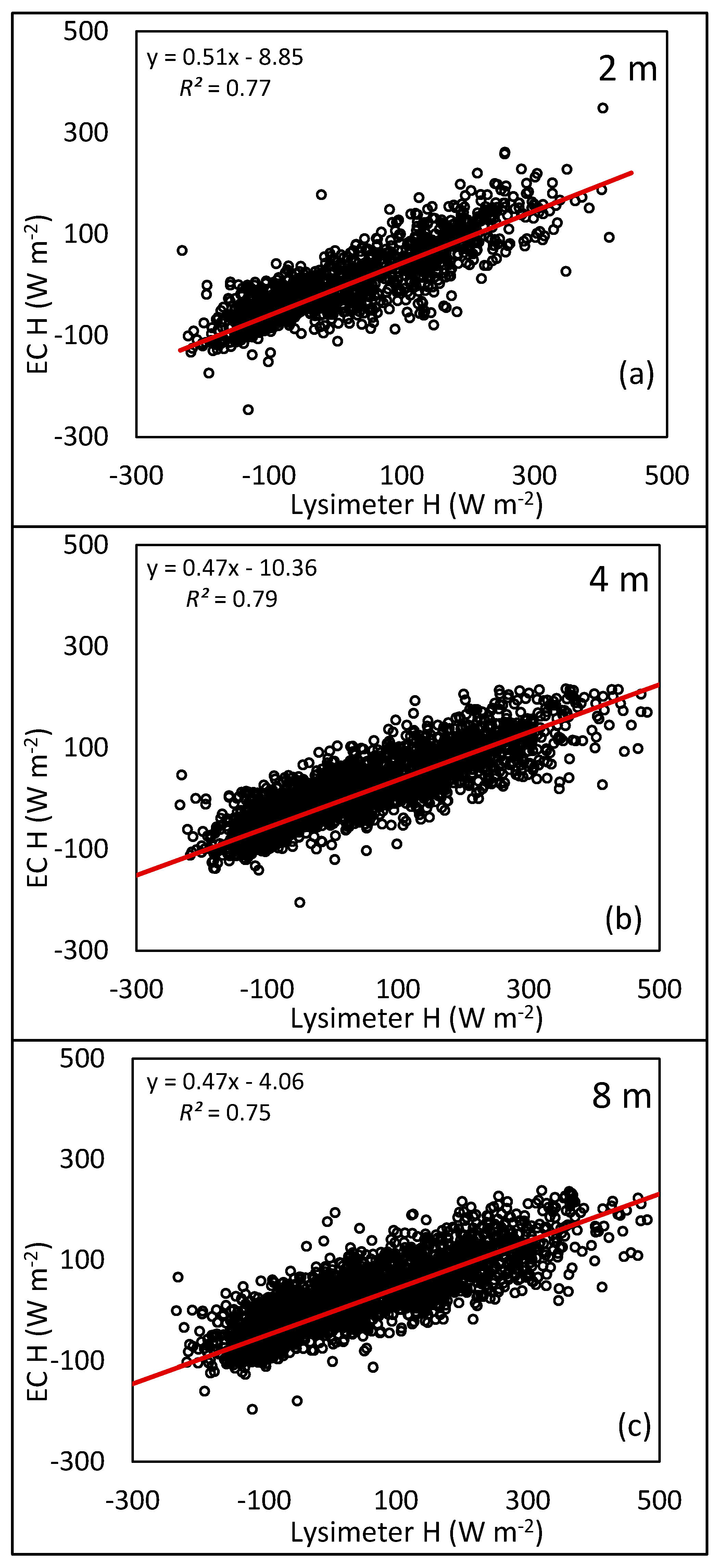
3.2. Sensible Heat Flux

H from EC underestimated H from the lysimeter by approximately 50% (see Figure 4). The RMSE was 55.5, 63.8, and 70.4 W m⁻² for the 2 m, 4 m, and 8 m sensors, respectively. Calculating the %RMSE was more difficult with H since values can be positive or negative; therefore, the absolute values for H were also used to calculate RMSE and %RMSE. The 2 m, 4 m, and 8 m sensors had a %RMSE of 44.3, 54.0, and 54.4, respectively. The regression graphs show EC has a more limited range of values for H compared to the lysimeter, possibly indicating the lysimeter having a greater capacity to capture H dynamics.

Separating the data for H by crop height gave better results when the crop was taller. After the grain sorghum reached maximum height the %RMSE for H was 35.4, 45.6, and 47.1 for the 2 m, 4 m, and 8 m, respectively, producing a reduction in %RMSE of 20.1, 15.6, and 13.4%, respectively. Although the lysimeter is considered very accurate for ET, it does not directly measure H. As H was calculated as the residual of the energy balance in this study, any error from the energy balance on the lysimeter would be included in the determination of H. Therefore, while the evaluation of H is included in this study, the accuracy of lysimeter H cannot easily be verified and the evaluation is presented for illustrative purposes.

3.3. Evapotranspiration

Average 30-min ET for the lysimeter and each EC system is presented in Figure 5. Each EC system followed a similar daily pattern as the lysimeter; however, each EC system overestimated ET. The three EC systems were similar for each half-hourly period throughout the day. Peak ET occurred around 13:00 for each system. Although the EC overestimated ET as compared to the lysimeter for the daytime hours, ET from EC was essentially zero for nighttime hours, while the lysimeter recorded small values for ET. The nighttime lysimeter measurements are in agreement with Tolk et al. [31], who showed small amounts of ET do occur at night.

Results from the regression analyses are presented in Figure 6 and

Table 2. Statistics from three eddy covariance systems evaluated against the lysimeter including root mean square error (RMSE), percent RMSE (%RMSE), correlation coefficient (R²), regression slope, regression intercept, and statistical p-value.

Sensor	RMSE	%RMSE	R2	Slope	Intercept	p-value
2 m	0.036	27.41	0.93	1.15	−0.02	<0.0001
4 m	0.036	26.68	0.91	1.17	−0.01	<0.0001
8 m	0.037	26.72	0.90	1.14	−0.02	<0.0001

. The slopes of the regression lines support the conclusion that EC overestimates ET as compared to the lysimeter with values above one. The slopes, intercepts, R², and RMSE values were similar between the three sensor heights (see Table 2). Error rates for ET (approximately 27%) are less than the closure error (approximately 35%) by regression slope indicating that although EC may have EB closure errors, EC may yield better results for ET after corrections and distributing residual energy by preserving the Bowen ratio. The large errors found in H based on comparison with the lysimeter indicate there is likely error in the Bowen ratio; however, the magnitude of H is much lower than the magnitude of LE. Therefore, any error in the Bowen ratio should be relatively low and the Bowen ratio may still provide an acceptable ratio for distributing the residual energy.

Evaluating only the daytime ET showed improvement in %RMSE for all three sensor heights with %RMSE values of 21.9, 30.0, and 30.7 for the 2 m, 4 m, and 8 m sensors, respectively. Using the larger daytime values, the magnitude of the RMSE increased for all sensors (i.e., 0.036 to 0.044 for the 2 m); however, the %RMSE decreased in each case, further illustrating the benefit of using relative differences in addition to error magnitudes. Removing the nighttime data still contained aggregated data points around the origin with overestimation of ET at higher values and a slight underestimation at values near zero.

RMSE and %RMSE values for ET from the three EC sensor heights separated by crop height are presented in

Table 3. RMSE and %RMSE for evapotranspiration separated by period of crop height.

Sensor	All Season	0.54 m	0.80 m	0.91 m	1.07 m	1.1 m	<1.13 m	1.13 m
2 m RMSE	0.036	0.037	0.037	0.038	0.034	0.033	0.038	0.032
4 m RMSE	0.036	0.038	0.039	0.036	0.035	0.032	0.039	0.037
8 m RMSE	0.037	0.038	0.038	0.038	0.034	0.032	0.039	0.039
2 m %RMSE	27.41	26.94	23.53	28.06	25.60	27.02	27.44	25.81
4 m %RMSE	26.68	26.33	23.16	26.18	26.40	25.98	27.41	43.54
8 m %RMSE	26.72	25.72	23.99	27.12	24.71	25.61	27.54	44.89

. Mean separation testing using the Student’s T method showed no significant differences between sensor heights for RMSE or %RMSE; however, a significant difference was found between %RMSE for the period after maximum plant height of 1.13 m was achieved and all periods prior. The 2 m sensor is an exception where the period after maximum plant height has a lower %RMSE; however, this sensor suffered a malfunction on 13 September 2015 yielding only 19 days of data for this period. The results from the 4 m and 8 m sensors show the %RMSE for ET from EC is less early in the growing season when sorghum plants are still actively growing. Further, separating the period after maximum plant height was reached by seven-day intervals (nine total weekly periods) showed the last four weeks (28 September–29 October) of the 2015 growing season had much higher %RMSE values, ranging from 78–90. ANOVA results showed each weekly period was significantly different with all p-values < 0.0001. These data show ET error is greatest at the end of the growing season during grain fill.

Finally, aggregating the half-hourly data to daily values improved results for ET and reduced %RMSE values to 16.04, 10.59, and 13.72 for the 2 m, 4 m, and 8 m sensors, respectively. The summed daily data drastically reduced the error rates, by as much as 50% in the case of the 4 m sensor. The decrease in error when summing the data is likely due to various cases of overestimation and underestimation evening out when the data are summed due to the trade-off between overestimation during daytime and underestimation during nighttime. Periods of overestimation and underestimation could be the result of a time lag between the measurements from EC and physical processes required to create a change in mass on the lysimeter. Although the 30-min averaging interval is considered the most representative time period for EC flux calculation, heat and energy transport often experience a time lag at rapid time scales as energy moves along the gradient. This time lag may contribute to greater error at half-hourly intervals but may be better accounted for in the daily sums.

4. Discussion

Results from this study over grain sorghum agree with a previous EC study at the CPRL over cotton (Gossypium hirsutum) by Chavez et al. [32]. They found EB closure errors of 46% and 27% for two EC systems installed on the lysimeter fields (denoted EC1 and EC2) for a 24-h time-step and 22% and 27% closure error, respectively, during daytime. This study showed similar EB closure error at 35% using the 24-h time interval. Evaluating the H, they found underestimations of 28% and 45% for the 24-h period and 35% and 37% for the daytime, similar to the 50% in this study. They also compared ET calculated from EC to lysimeter measured ET and found under predictions of 30% and 38% in ET from EC1 and EC2, respectively, but results improved to 24 and 22% after forcing EB closure. This study showed an overestimation of 27% sorghum ET.

In a study by Alfieri et al. [33], two EC systems were installed in each of two lysimeter fields at the CPRL to determine the effects from advection. When considering the full 24-h period, differences in LE from EC systems and lysimeters ranged from 49 to 76 W m⁻², which is similar to the ~50 W m⁻² for grain sorghum in this study. The EB closure percentage for the four EC systems ranged from 74% to 87%, which is slightly higher than the 65% in this study. Investigating the closure error causes, they found that the effect of advection on flux measurements was typically less than 20 W m⁻², although there were two days where the advection effect was larger than 100 W m⁻².

Perez-Priego et al. [34] showed EC to underestimate LE as compared to a lysimeter for an oak tree-grass savannah in a Mediterranean climate. Their analysis showed the selection of correction methods can greatly impact EC results. One example given by Perez-Priego et al. [34] showed applying the angle-of-attack correction changed the EB closure slope from 0.92 to 1.07.

As many agricultural EC studies either analyze several non-consecutive days or a relatively short section of the growing season, this study provided the opportunity for additional analysis with complete data from early in the growing season to harvest. The ability to analyze sections of the growing season to investigate in-season dynamics of H and LE showed that errors in EC are not consistent throughout the growing season.

The inconsistency throughout the growing season in this study differs from the results presented by Ding et al. [35] who showed errors of ±15% for each maize crop growth stage. They separated results into seedling, shooting, heading, filling, and maturity stages with each stage encompassing 17–45 days. The main difference in the methodology between Ding et al. [35] and this study is that they used plastic film to suppress evaporation and flood irrigation. With the potential for evaporation reduced, the microclimate of the crop canopy would likely have been different than this study, potentially reducing the energy available for storage in the plant canopy. From the analysis of the data by crop height, the results showed EB closure was better when the crop was smaller and poorer when more biomass was present on the surface. This indicates canopy heat storage may be one of the sources of error in EC-derived energy fluxes.

In terms of water for irrigation, using the overestimated ET in irrigation scheduling would lead to overapplication of water. Using the northern THP as an example, a 10% overestimation, resulting in a 10% overapplication for all irrigated acres, the annual water used for irrigation would increase by over 313 million m³ (254,000 ac-ft) based on the TAMA water demand model [1]. The water use applied to the scale of irrigated acres highlights the necessity of highly accurate ET data.

5. Conclusions

This study involved EC systems installed over irrigated grain sorghum at heights of 2.5, 4.5, and 8.5 m for the 2015 summer growing season. Results showed EC underestimated H and overestimated LE (as indicated by ET). However, the underestimation of H was not equal to the overestimation of LE. EB closure was approximately 65%, due in part to the 50% error in H. Separating EB closure analysis by crop height showed closure was greater earlier in the season and lower after the crop reached maximum height. The closure discrepancy could be caused by unaccounted energy stored in the plant canopy.

These results showing less error in LE also indicate that ET from EC may have better accuracy than would be indicated by EB closure. Half-hourly ET error rates of 20%–30% may be greater than desired for many water management applications; however, the results of this study show certain periods, namely the later vegetative and early reproductive stages, have less error than the total growing season. For irrigation management, the late vegetative and early reproductive stages correspond to the greatest water use in many crops, including grain sorghum. Therefore, EC could potentially provide the best accuracy during the periods of peak water demand.

Moreover, since error rates are drastically reduced when summed to daily values, EC may provide more potential for use in agricultural water management as most management practices, including irrigation scheduling, are performed at daily or longer time-steps. For most water availability and modeling applications, data could potentially be aggregated to weekly or monthly time steps that could further reduce error. With error in daily ET of 10%–15%, EC shows potential for many uses in agricultural water management.

6. Disclaimer

The use of trade, firm, or corporation names in this publication (or page) is for the information and convenience of the reader. Such use does not constitute an official endorsement or approval by the United States Department of Agriculture or the Agricultural Research Service of any product or service to the exclusion of others that may be suitable.