Soil Water Content and High-Resolution Imagery for Precision Irrigation: Maize Yield

Abstract

Improvement in water use efficiency of crops is a key component in addressing the increasing global water demand. The time and depth of the soil water monitoring are essential when defining the amount of water to be applied to irrigated crops. Precision irrigation (PI) is a relatively new concept in agriculture, and it provides a vast potential for enhancing water use efficiency, while maintaining or increasing grain yield. Neutron probes (NPs) have consistently been used as a robust and accurate method to estimate soil water content (SWC). Remote sensing derived vegetation indices have been successfully used to estimate variability of Leaf Area Index and biomass, which are related to root water uptake. Crop yield has not been evaluated on a basis of SWC, as explained by NPs in time and at different depths. The objectives of this study were (1) to determine the optimal time and depth of SWC and its relationship to maize grain yield (2) to determine if satellite-derived vegetation indices coupled with SWC could further improve the relationship between maize grain yield and SWC. Soil water and remote sensing data were collected throughout the crop season and analyzed. The results from the automated model selection of SWC readings, used to assess maize yield, consistently selected three dates spread around reproductive growth stages for most depths (p value < 0.05). SWC readings at the 90 cm depth had the highest correlation with maize yield, followed closely by the 120 cm. When coupled with remote sensing data, models improved by adding vegetation indices representing the crop health status at V9, right before tasseling. Thus, SWC monitoring at reproductive stages combined with vegetation indices could be a tool for improving maize irrigation management.

1. Introduction

An accurate understanding of soil water content behavior is important for soil hydrological research in areas, such as irrigation scheduling and site-specific agriculture [1]. Part of the solution for sustainable productivity is the improvement of water use efficiency. It is important to irrigate when the yield response to water is at maximum. Plant water use efficiency (WUE) is defined as the amount of carbon gained per unit of water and used on a unit of land area [2]. The impact of a water deficit on the WUE varies throughout the growing season depending on how sensitive the crop is at that specific growth stage. Therefore, both, the amount of water availability, as well as the timing of water availability, are critical.

Water extraction is not uniform across a field [3], which leads to the need for an investigation on the effect of spatial distribution of vegetation and its influence on the spatial pattern of soil water content. Hupet and Vanclooster [1] discussed a non-negligible role of the evapotranspiration of plants in the soil moisture patterns for the shallow layers. However, their conclusions were different in experiments that studied deeper soil water readings [4]. Little research has focused on the importance or explanatory significance of soil water content readings at different depths. Longchamps, Khosla, Reich and Gui [3] proposed the use of variable rate irrigation only when the roots are deep enough, and soil water content shows more stable spatial patterns.

Given these conditions, it may be necessary to add a crop attribute to account for the spatial variability in water consumption. Vegetation indices derived, from remote sensing, have been successfully used to estimate the spatial variability of crop LAI and biomass [5] and yield [6]. One of the oldest and most popular indices is the Normalized Difference Vegetation Index (NDVI) [7]. However, when LAI in maize canopies are higher than 2.0, NDVI is normally insensitive to changes [8]. Viña, et al. [9] found that among various vegetation indices evaluated, the Red-Edge Chlorophyll Index (RECI) could also be used to accurately estimate LAI for crop canopies ranging from 0 to more than 6 m² of vegetation per m² of soil. Delegido, et al. [10] found that the Red-Edge Normalized Difference Vegetation Index (RENDVI) does not saturate at high LAI values, and is strongly related to the physiological status of the plant, for a wide range of crops and conditions.

The review of current literature indicates that soil water content (SWC) and grain yield relationship has not been thoroughly studied from a time and depth perspective, and least of all at the field scale. Hassan-Esfahani, et al. [11] presented one of the few studies on the estimation of SWC at the root zone, using high resolution remote sensing data, and demonstrated the potential of vegetation indices to estimate SWC, but did not link SWC to crop yield. A recent review paper have identified the need for a combined soil-based and crop-based approach to better estimate crop water needs [12]. The link between SWC, high resolution vegetation indices, and yield may be key to developing agronomically sound precision irrigation strategies, suitable for precision agricultural systems. The hypothesis of this study is that soil water content, measured at different times and depths is spatially related to grain yield. This could provide useful information for developing and installing soil water sensors for the field scale water management. With a stronger spatial dependency of the soil water content (SWC) at greater depth, fewer sensor locations would be necessary to measure soil moisture and characterize the soil water content profile.

The objectives of this study were (1) to determine the optimal time and depth of soil water measurements and its relationship to maize grain yield at the field scale, and (2) to determine whether satellite-derived vegetation indices, coupled with soil water measurements, could further improve the relationship between maize grain yield and soil water measurements.

2. Materials and Methods

2.1. Study Sites

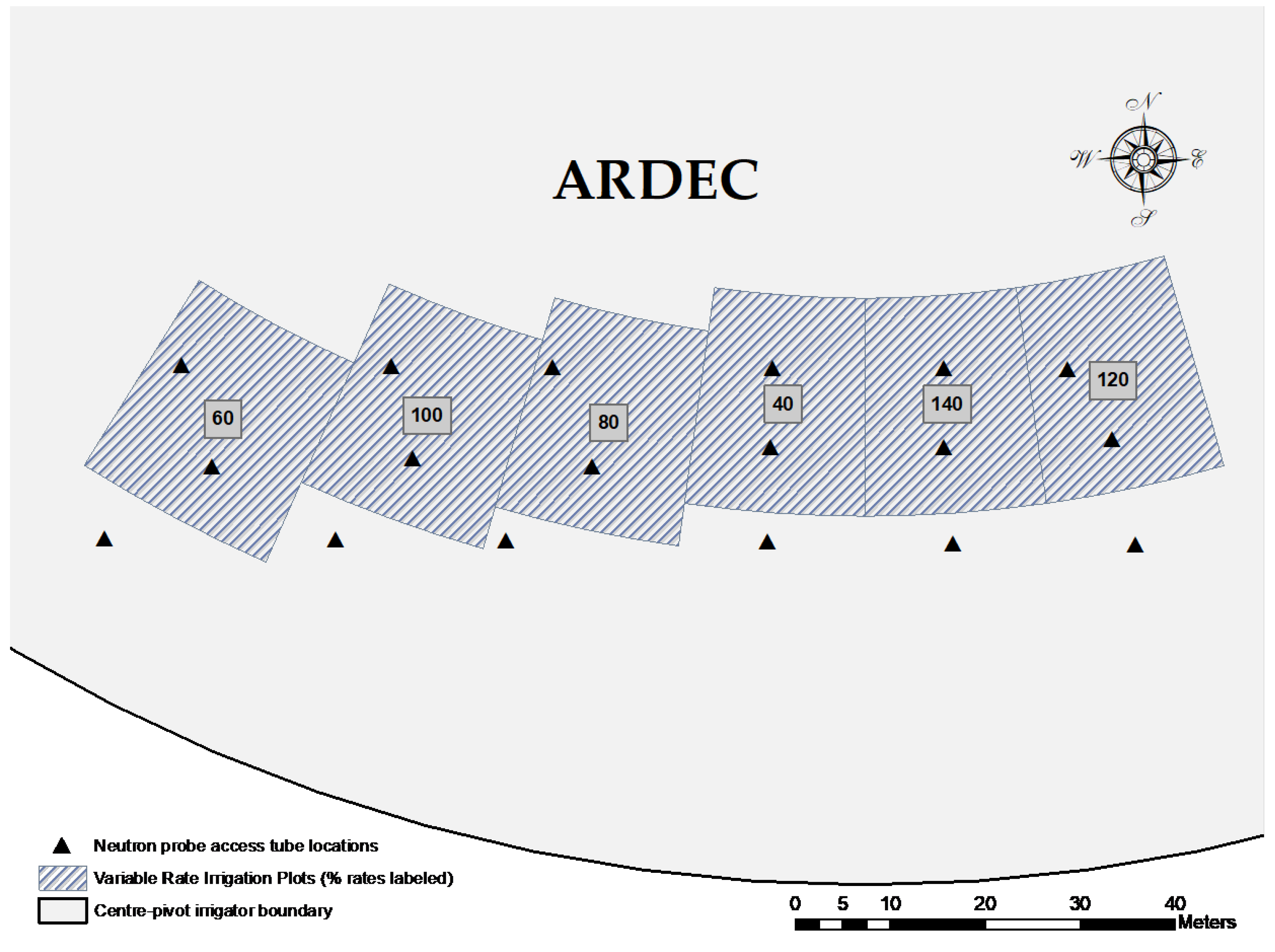
This study was conducted in 2015 at the Agricultural Research Development & Education Center (ARDEC), Fort Collins, CO, USA (40°39′57.4″ N, 104°59′53.1″ W, Figure 1). This site was under a continuous maize cropping system and irrigated by a center-pivot irrigation system with variable rate prescription capability. The soil type is a Kim loam (Fine-loamy, mixed, active, calcareous, mesic Ustic Torriorthents). These soils are characterized as being very deep, well drained, with 1 to 3 percent slopes [13].

2.2. Soil Water Data Collection

Soil water data was collected at five soil depths (30, 60, 90, 120, and 150 cm) utilizing a neutron probe (Model 503 DR Hydroprobe, CPN International, Martinez, CA). In addition to the original five NP readings, three average SWC for depths 30–60, 30–90 and 30–150 cm were computed, assuming constant bulk density of soil for those depths. The NP readings were taken 21 times during the crop growing season, on a bi-weekly basis, from July 22th to September 24th. A total of 18 access tubes were installed (Figure 1), and their geo-location was logged, using a differential-corrected Trimble^TM Ag 114 global position system (DGPS) unit. Access tubes were positioned within crop rows, and 12 of the 18 were located under a variable rate irrigation (VRI) (Figure 1). The reason for the access tubes distribution was to measure variability in water availability with irrigation applications of 40%, 60%, 80%, 100%, 120%, and 140% of the crop evapotranspiration (ET), while the uniform rate was always 100% of the ET. Estimated ET requirements, or the amount needed to replenish water used by the plants and lost to evaporation, are based on weather conditions such as solar radiation, windspeed, and humidity. For information on calculating crop water requirements, refer to [14]. Every time the NP is used, a standard measurement was acquired with the sensor located in the probe enclosure to obtain a “count ratio” which consists of the division of the actual field readings by the standard.

2.3. Remote Sensing Data

Satellite images were obtained by the RapidEye system (BlackBridge, Berlin, Germany), for a total of seven dates, distributed across the crop growing season. The imagery was corrected for radiometric error and geo-rectified by the provider, FarmLogs (Ann Arbor, MI, USA). Three different vegetation indices (NDVI, RECI, and RENDVI) were calculated, thus a total of 21 high-resolution maps (at 5 m spatial resolution) were obtained (

Table 1. Vegetation indices evaluated in the study.

Index †	Formulation ‡	Source	Resolution	Reference
NDVI	$\frac{\mathrm{NIR}-\mathrm{Red}}{\mathrm{NIR}+\mathrm{Red}}$	RapidEye	5 m	[7]
RECI	$\frac{\mathrm{NIR}}{\mathrm{Red}\_\mathrm{edge}}-1$	RapidEye	5 m	[15,16]
RENDVI	$\frac{\mathrm{NIR}-\mathrm{Red}\_\mathrm{edge}}{\mathrm{NIR}+\mathrm{Red}\_\mathrm{edge}}$	RapidEye	5 m	[10]
EVI	2.5 × $\frac{\mathrm{NIR}-\mathrm{Red}}{1+\mathrm{NIR}+6\times \mathrm{Red}-7.5\times \mathrm{Blue}}$	MODIS	250 m	[17]

^† NDVI, Normalized Difference Vegetation Index; RECI, Red Edge Chlorophyll Index; RENDVI, Red Edge Normalized Difference Vegetation Index; EVI, Enhanced Vegetation Index; ^‡ The NDVI, RECI and RENDVI formulation names NIR, Red, Red edge refers to RapidEye’s band 5 (760–850 nm), band 3 (630–685 nm), and band 4 (690–730 nm), respectively. The EVI formulation names NIR, Red, Blue refers to MODIS’s band 2 (841–876 nm), band 1 (620–670 nm), and band 3 (459–479 nm), respectively.

). Ancillary vegetation indices from the Moderate Resolution Imaging Spectroradiometer (MODIS) sensors (250 m spatial resolution) were provided by The Oak Ridge National Laboratory Distributed Active Archive Center (ORNL DAAC). The Enhanced Vegetation Index (EVI) was used given its high sensitivity over dense maize vegetation conditions and less interference of the soil background (Table 1). Ancillary imagery were obtained every 16 days for the 2015 season, resulting in a total of 11 vegetation indices.

2.4. Crop Yield Data

The site was harvested at maize physiological maturity. Aboveground biomass was harvested by hand around the neutron probe locations and weighed. Each sampled point consisted of harvesting maize ears on 4 lines, of 3 m each, surrounding the neutron probe access tube locations.

2.5. Statistical Analysis

Data analysis was performed using the R statistical software [18]. Correlation analysis (Pearson’s Correlation with p value = 0.05) was performed to study the relationship between SWC, remote sensing data, and yield values. Further, polynomial models were tested given the quadratic relationship between SWC and yield shown in the literature [19]. Coefficient of determination of the quadratic relationship between SWC and maize yield was obtained by fitting polynomial models to the SWC values against yield using the “poly” function, R package “stats” [18]. Regression and analysis of variance were also performed by fitting linear models to assess maize yield using SWC, and SWC coupled with remote sensing data. Automated model selection was performed with the “dredge” function, R package “MuMIn” [20], which generated a list of all possible models sorted by explanatory power. The corrected version of the Akaike Information Criteria (AICc), which adjusts for finite sample sizes, guided selection of the preferred model [21]. Comparison of full and simpler models for significant differences were executed using the “ANOVA” function from the base R package (p value = 0.05).

2.6. Best Model’s Selection

Automated model selection computes every possible predictor combination (soil water measurements) to estimate the response variable (maize yield). Therefore, due to restrictions in the number of degrees of freedom for modeling, filtering the available dates by highest correlations with yield, was necessary. Only the dates, with correlation coefficients higher than 0.5, were used. Likewise, to decrease the number of predictors and increase the statistical power, only linear regression models were included.

2.6.1. Best Dates Model

Automated model selection was performed for each of the five depths (i.e., 30, 60, 90, 120, and 150 cm) to detect which dates were more often correlated across all models. In other words, in search for the dates when correlation with yield was the strongest.

2.6.2. Best Depth Models

Best Depth for Each Date Model:

For each of the most relevant dates (correlation coefficients with yield higher than 0.5), automated model selection was performed, using the depths as independent variables (from 30 to 150 cm), in search for the most frequent depths when correlation with yield was strongest.

Best Depth Including All Relevant Date Model:

The r² values were calculated using only the most relevant dates (i.e., correlation coefficients with yield higher than 0.5) for each depth (from 30 to 150 cm). The purpose was to compare full models and estimate the potential explanatory power for each depth.

2.6.3. Imagery Model

Automated model selection was used to test the inclusion of vegetation indices as plant soil water uptake explanatory variables to the chosen dates in the previous SWC “best dates model”. The average soil water content for depths down to 150 cm (mean of the entire profile) were used as the base model. For imagery of the seven available dates, one vegetation index at a time was combined with the base model to assess yield.

3. Results

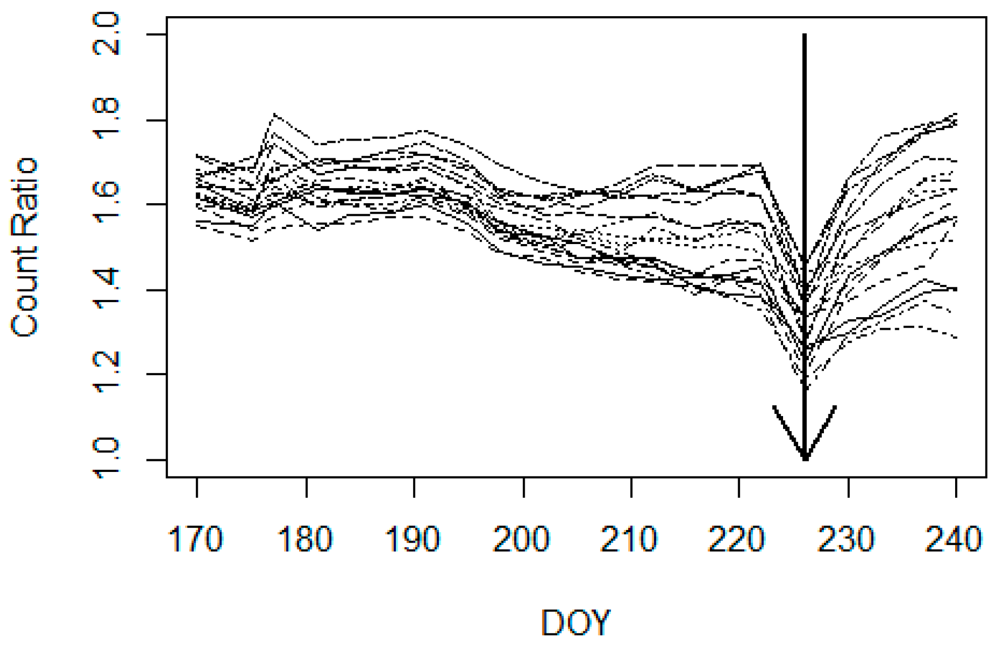
Maize tasseling was observed around 8 August (DOY 220). The mean yield value was 14.5 Mg ha⁻¹ and yield ranged from 11.2 Mg ha⁻¹ to 15.8 Mg ha⁻¹. Neutron count ratios (NCR) ranged from 1.10 to 1.97 across all dates and depths (higher values were directly related to SWC). The polynomial transformation of the NCR values improved the explanation of the yield variance, and therefore, were used as inputs for further analyses. Multiple significant coefficients of determination (r²) from the quadratic model between NCR readings and maize yield were observed (

Table 2. Coefficient of determination (r²) between neutron probe (NP) and yield at different depths and days of the year (DOY). The r² was indicated when a significant (p value < 0.05) correlation coefficients was observed, and non-significant relationship were indicated by a hyphen (-).

NP DOY †	Depth
	30 cm	60 cm	90 cm	120 cm	150 cm	$\stackrel{-}{\mathbf{X}}$ 30–60 cm	$\stackrel{-}{\mathbf{X}}$ 30–90 cm	$\stackrel{-}{\mathbf{X}}$ 30–150 cm
170	-	-	-	-	-	-	-	-
175	-	-	-	-	-	-	-	-
177	-	-	-	-	-	-	-	-
181	-	-	-	-	-	-	-	-
184	-	-	-	-	-	-	-	-
188	-	-	-	-	-	-	-	-
191	-	-	-	-	-	-	-	-
195	-	-	-	-	-	-	-	-
198	-	-	-	-	-	-	-	-
202	-	-	-	-	-	-	-	-
205	0.36	-	-	-	-	-	-	-
209	0.48	-	-	-	-	-	-	-
212	0.62	0.33	-	-	-	-	0.38	-
216	0.66	0.37	-	-	-	-	0.46	0.45
219	-	0.50	-	0.34	0.56	0.47	0.37	0.44
222	0.70	0.48	-	-	0.50	0.70	0.57	0.58
226	0.36	0.48	0.62	0.66	-	0.43	0.54	0.58
230	0.71	0.54	-	0.64	0.41	0.74	0.60	0.64
233	0.70	0.59	0.44	0.61	0.60	0.76	0.72	0.74
237	0.65	0.59	0.46	0.57	0.74	0.74	0.72	0.75
240	0.72	0.58	0.57	0.76	0.70	0.77	0.75	0.76

^† Neutron probe Day of year measurement.

). Stronger correlations between SWC and yield at the beginning of tasseling, validate that, during this stage, the impact of soil water levels on yield is highest. There was a notable decrease in the neutron probe reading values one week after the start of tasseling, (DOY 226), indicated with a bold arrow in Figure 2.

3.1. Best Dates Model

From the coefficients of determination (Table 2), only the NCR from the 11 latest dates (i.e., from DOY 205 to DOY 240) were significant.

Table 3. Dates selected by the best model for each depth. Total number of significant contributions to the model across soil depths for each day of the year is indicated in the bottom row of the table. Dates selected by the best model are highlighted in bold.

Depth	NP DOY †											r2	p Value
	205	209	212	216	219	222	226	230	233	237	240
30 cm	-	-	X	-	X	-	-	-	-	X	-	0.83	<0.001
60 cm	-	-	-	-	-	X	X	-	-	-	X	0.72	<0.001
90 cm	-	-	-	-	-	X	X	-	-	X	-	0.80	<0.001
120 cm	-	X	-	-	X	X	X	X	-	-	-	0.89	<0.001
150 cm	-	X	-	-	-	-	-	-	-	X	-	0.64	<0.001
Total	0	2	1	0	2	3	3	1	0	3	1	-	-

^† Neutron probe Day of year measurement.

shows the dates selected by the best models to explain maize yield at each measurement depth. The SWC measurements from the DOY 222, 226, and 237 had the highest number of significant contributions to the model across soil depths with 3 of 5 possible appearances each. The first variable (DOY 222) coincides with the beginning of tasseling, which was observed for the first time at DOY 220. The next variable (DOY 226) coincides with a noticeable decrease in soil water reading values, when maize plant water uptake is expected to be at the maximum rate, due to high demand [22]. Finally, the last variable (DOY 237) provided important information about the water status at the end of the reproductive stages, when yield is still being defined.

3.2. Best Depth Models

3.2.1. Best Depth for Each Date Model:

Table 4. Neutron count ratios acquired on various days of the year (DOY) at specific soil depths and corresponding coefficients of determination for the best model to assess maize yield for each. The most often selected soil depth is highlighted in bold.

NP † DOY †	Soil Depth					r2	p Value
	30 cm	60 cm	90 cm	120 cm	150 cm
205	X	-	-	-	-	0.30	0.02
209	X	-	-	-	-	0.41	0.00
212	X	-	X	-	-	0.60	0.00
216	X	-	-	-	-	0.59	0.00
219	-	-	-	X	-	0.34	0.01
222	X	-	-	-	-	0.63	0.00
226	-	-	-	X	-	0.59	0.00
230	-	-	X	X	-	0.67	0.00
233	X	-	-	-	-	0.59	0.00
237	X	-	-	-	-	0.65	0.00
240	X	-	-	-	-	0.71	0.00
Total	8	0	2	3	0

^† Neutron probe Day of year measurement.

shows the depths selected by the best models to explain maize yield at each measurement date. The explanatory power of the models strongly depends on the date of acquisition, with r² values ranging from 0.30 (DOY 205) to 0.71 (DOY 240). Nevertheless, the 30 cm soil depth SWC reading appears to be the most explicative one, for 8 of the 11 dates (73% of the time).

3.2.2. Best Depth for All Relevant Dates Model:

The r² values were calculated for SWC for each soil depth, with all 11 dates included as model predictors (

Table 5. Soil depths and corresponding coefficients of determination for the model that included all dates on which soil water content was acquired to assess maize yield.

Soil Depth	r2
30 cm	0.85
60 cm	-
90 cm	0.93
120 cm	0.92
150 cm	-

The r² was indicated when a significant (p value < 0.05) correlation coefficient was observed, and non-significant relationship were indicated by a hyphen (-).

). The SWC readings at 90 cm soil depth had the strongest relationship (r² = 0.93) with maize yield.

3.3. Imagery Model

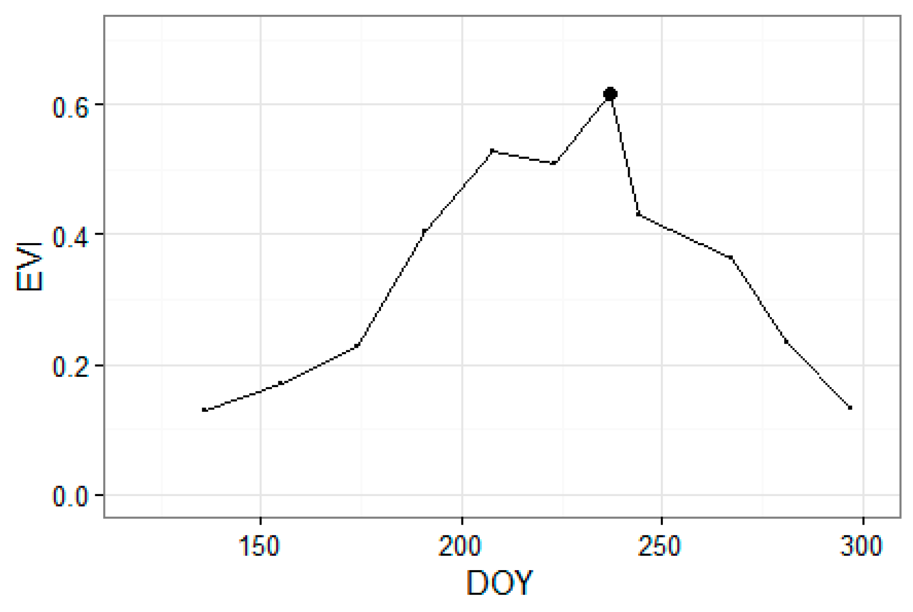
The temporal variation of biomass, described by the EVI, is depicted in Figure 3. The peak growth period occurred around DOY 237. Figure 4 (40°39′57.4″ N, 104°59′53.1″ W) illustrates the spatial variability in crop biomass, as characterized by the three vegetation indices, acquired near the peak growth stages.

The NDVI ranged from 0.11 to 0.79, RECI ranged from 0.21 to 3.53, and RENDVI ranged from 0.06 to 0.45, across all dates for which SWC was acquired. The DOY 221 was a cloudy day and the three indices had to be discarded due to a substantial cloud coverage over the ground cover. The RECI and RENDVI values for DOY 242 imagery (i.e., latest imagery acquired for the season) were the only ones that showed significant correlation with maize grain yield (

Table 6. Vegetation indices, day of year (DOY) and corresponding correlations coefficient in relation to maize yield.

Vegetation Index †	Correlation Coefficient
	DOY
	155	164	178	192	204	242
NDVI	-	-	-	-	-	-
RECI	-	-	-	-	-	0.72
RENDVI	-	-	-	-	-	0.63

^† Significant (p value < 0.05) correlation coefficients are reported and non-significant correlation are indicated with a hyphen (-).

).

The significant dates identified in the best dates model (3.1) for the average of the entire soil profile were DOY 219, 226, and 237. The three NP readings dates mentioned were set to be consistently part of the output models, and the six available imagery dates, one index at a time, were tested for the improvement of the best date model. Outputs from the automated model selection for NDVI, RECI and RENDVI are shown on

Table 7. Results from the automated model selection for the imagery models. Selected variables of the best model for each index are indicated with an X. Numbers next to variables indicate the corresponding Day of the year.

NDVI † Model
NP 219	NP 226	NP 237	NDVI 155	NDVI 164	NDVI 178	NDVI 192	NDVI 204	NDVI 242	r2	AICc #
X	X	X	-	-	-	-	-	-	0.77	297.3
RECI ‡ Model
NP 219	NP 226	NP 237	RECI 155	RECI 164	RECI 178	RECI 192	RECI 204	RECI 242	r2	AICc
X	X	X	-	-	-	-	X	-	0.84	294.9
RENDVI § Model
NP 219	NP 226	NP 237	RENDVI 155	RENDVI 164	RENDVI 178	RENDVI 192	RENDVI 204	RENDVI 242	r2	AICc
X	X	X	-	-	-	-	X	-	0.83	296.4

^† Normalized Difference Vegetation Index Day of year; ^‡ Red-edge Chlorophyll Index Day of year; ^§ Red-edge Normalized Difference Vegetation Index Day of year; ¶ Neutron probe Day of the year; # corrected Akaike Information Criteria.

.

None of the NDVI values, calculated for six dates, were selected to improve the reduced model (SWC-only model), therefore the best model remained the same as the “best dates model” (r² = 0.77, AICc = 297.3). The RECI and RENDVI automated model selection included the indices of DOY 204 in both cases and was a significant (p value < 0.05) improvement to the SWC-only model. The wide range of values of RECI and sensitivity of RENDVI over NDVI is noticeable in Figure 4, where lower contrast is observed for the latter index. The NDVI failed to explain maize biomass variability, probably due to saturation of this index at high leaf area index values, as previously suggested [23].

4. Discussion

The deeper SWC readings (i.e., 90 to 150 cm) showed significant relationships with maize yield later during the growing season. Similar trends were detected by Hupet and Vanclooster (2002), explaining that plants’ water uptake affects the deeper soil layers (50 to 100 cm), as a result of the transpiration from the well developed maize crop, combined with a high climatic demand. The common wisdom among farmers in Colorado (personal communication) is that ample irrigation at the beginning of the crop season builds a storage of water in the soil to be used later in the season when water requirements are the highest, known as soil water “banking” [24]. The results from this study seem to provide a scientific basis to support farmer’s technique. It was observed that, generally, in the crop growing season, shallow SWC was the most important parameter for yield determination. However, at early to mid-reproductive crop growth stages, when crop water demand is the highest, deeper SWC was crucial and played the largest role in the grain yield formation. Furthermore, a significant decrease in SWC of the entire profile was observed one week after the onset of tasseling.

The findings from this study suggest that, at the tasseling growth stage (VT), there is a narrow window of perhaps five days, when the SWC of the entire profile is critical. During this period, root water uptake rate might be remarkably high, and depending on the soil type, the irrigation may not be able to physically keep up with the crop water consumption [24]. Therefore, deeper soil water availability might be the largest yield limiting factor at this stage, and accumulating water in the soil profile (e.g., water “banking”) could be a feasible solution. This suggests that site-specific irrigation management, targeting spatially variable SWC, would have a maximum impact later in the season, when water patterns are more related to crop’s yield. Likewise, Longchamps, et al. [3], suggested that variable rate irrigation may be more practical when roots are deep enough (below 45 cm), where SWC spatial patterns are more stable. Uniform irrigation may be adequate for most of the growing season, but aiming for site-specific amounts of water during the period bracketing, flowering could further improve the efficiency of the irrigation.

The first important component found in this study was the neutron probe readings acquired around the reproductive stage (DOY 222, 226 and 237), which successfully described the soil water availability during the critical growth period (Table 3). The second component was the significant modeling contribution of RECI or RENDVI image of the crop before tasseling (DOY 204), which corresponded to the V9 (9-leaf) growth stage of maize (Table 7). At this stage, maize already had nine expanded leaves and was at the beginning of the most resource-demanding period of its life-cycle. Root depth, leaf area, and water use increase rapidly during this period, reaching peak daily water use rates during pollination [22]. A water stress during this period would have the greatest impact on the crop yield [22]. Therefore, an image acquired at V9 growth stage of maize is a snapshot of the plant’s potential to use all of the available resources during the upcoming critical growth period, which defines most of the grain yield. The better performance of RECI and RENDVI indices explain the higher biomass amounts, which may be due to the inclusion of the red edge band instead of the red band in the NDVI. While the red band capitalizes on the sensitivity of the vegetation, the red edge band responds to small changes in LAI, the latter being located between the main absorption and reflection peaks of the spectrum [25]. The red edge band is spectrally located between the red and NIR band, where the reflectance highly increases from the red portion towards the NIR plateau for green vegetation [26]. Viña, Gitelson, Nguy-Robertson, and Peng [9] tested the performance of NDVI, RECI, and MERIS Terrestrial Chlorophyll Index (MTCI), which also includes the red edge band, to estimate maize and soybean LAI. The RECI and MTCI exhibited more sensitivity to moderate to high LAI, than the widely used NDVI. Depending on the development, growth, type of crop, and the minimum requirements of the variability assessment, the widely used NDVI may not always be the best index. Indices, such as those including the red edge band in their formulation, could be a potential replacement to NDVI in scenarios where the LAI values are high and NDVI saturates.

Practical Implications

Our results suggest that the superficial soil layers would be the most appropriate to monitor, when the purpose of soil water measurements is to ascertain crop water requirements throughout the crop growing season. This would be especially useful for soil water monitoring when only a limited number of sensors can be installed at a single soil depth. If the depth of measurement can change during the growing season, in particular during the early-mid reproductive growth period, deeper SWC monitoring would be more appropriate for a more efficient irrigation management.

The imagery model, which is a combination of soil water measurements and remote sensing data, provides some new insights on how to develop high frequency soil water maps. Frequent maps of the vegetation cover as estimated by remote sensing combined with maps of the crop potential yield could provide useful information about the plant’s water status for the entire field. Such maps could be used to address the high temporal variability previously reported in the SWC at the soil surface [1,3]. Soil moisture probes could be used to acquire data on SWC variability at deeper soil depths which tends to be relatively stable [3]. Combining the crop imagery with deep soil moisture probe data may render possible the estimation of SWC of the entire root zone soil profile (0–100 cm).

The advent of new technologies (e.g., drones, nano-satellites), makes high temporal and/or spatial resolution imagery of fields, accessible and easier than ever. Santesteban, et al. [27] tested new light-weighted thermal cameras to estimate the plant water status within a vineyard, with successful results. In addition, this information could be coupled with soil water management zones, which consists of different levels of available water-holding capacities across the field [28]. In sum, inter- and intra-zone variability could be more precisely described, representing valuable information for an optimal irrigation water management along the crop growing season. Nonetheless, further investigation, on how to precisely combine all the different sources of water information, has to be further studied.

5. Conclusions

Grain yield across a variable rate-irrigated maize field was shown to be related (r² up to 0.89) to the SWC, as measured by NP readings. When water was the main factor controlling grain yield, the importance of the SWC values, in space and depth, varied across the crop growing season. From the correlation analysis between single NP readings and yield values, there was a trend consisting of higher correlation (r² of 0.71 at DOY 240) after tasseling. Similarly, automated model selection chose NP reading dates spread around reproductive growth stages to best assess maize grain yield. During this period, deeper SWC readings had the strongest relationship with crop yield and may be the most limiting factor defining yield. However, if the goal is to characterize water requirements apart from the critical growth stages, the surface readings explained (p value < 0.05 for 8 out 11 dates) the maize yield most of the time. To enhance the maize yield prediction by SWC, vegetation indices were also included in an attempt to describe the plant biomass, which is highly related with the plant water uptake. The RECI and RENDVI proved to be significant additions to the SWC-only model, improving the grain yield assessment from an r² of 0.77 to 0.84 and 0.83, respectively (ANOVA test, p value < 0.05). The NDVI failed to improve the SWC-only model, suggesting that in order to account for the subtle differences in biomass, the red-edge-based vegetation indices may be a better solution. The results from this study showed that, different sources of information could be combined to obtain more accurate models of soil water content and maize yield at the field scale, appropriate for precision irrigation.

Future Work

The incorporation of soil water management zones could be significant in developing site-specific models, in order to account for spatial variability of the soil’s available water-holding capacity. Combined with newer remote sensing technologies (e.g., higher spatial and temporal resolution, thermal imagery), an enhanced characterization of the soil water status could be performed. All sources of information together, properly integrated, could become a powerful tool for an optimal irrigation management.

References

- Hupet, F.; Vanclooster, M. Intraseasonal dynamics of soil moisture variability within a small agricultural maize cropped field. J. Hydrol. 2002, 261, 86–101. [Google Scholar] [CrossRef]
- Steduto, P. Water use efficiency. In Sustainability of Irrigated Agriculture; Springer: New York, NY, USA, 1996; pp. 193–209. [Google Scholar]
- Longchamps, L.; Khosla, R.; Reich, R.; Gui, D. Spatial and temporal variability of soil water content in leveled fields. Soil Sci. Soc. Am. J. 2015, 79, 1446–1454. [Google Scholar] [CrossRef]
- Vachaud, G.; Passerat de Silans, A.; Balabanis, P.; Vauclin, M. Temporal stability of spatially measured soil water probability density function. Soil Sci. Soc. Am. J. 1985, 49, 822–828. [Google Scholar] [CrossRef]
- Wiegand, C.; Richardson, A.; Escobar, D.; Gerbermann, A. Vegetation indices in crop assessments. Remote Sens. Environ. 1991, 35, 105–119. [Google Scholar] [CrossRef]
- Ashcroft, P.; Catt, J.; Curran, P.; Munden, J.; Webster, R. The relation between reflected radiation and yield on the broadbalk winter wheat experiment. Remote Sens. 1990, 11, 1821–1836. [Google Scholar] [CrossRef]
- Rouse, J.; Haas, R.; Schell, J.; Deering, D. Monitoring vegetation systems in the great plains with erts. NASA Spec. Publ. 1974, 351, 309. [Google Scholar]
- Gitelson, A.A.; Viña, A.; Arkebauer, T.J.; Rundquist, D.C.; Keydan, G.; Leavitt, B. Remote estimation of leaf area index and green leaf biomass in maize canopies. Geophys. Res. Lett. 2003, 30. [Google Scholar] [CrossRef]
- Viña, A.; Gitelson, A.A.; Nguy-Robertson, A.L.; Peng, Y. Comparison of different vegetation indices for the remote assessment of green leaf area index of crops. Remote Sens. Environ. 2011, 115, 3468–3478. [Google Scholar] [CrossRef]
- Delegido, J.; Verrelst, J.; Meza, C.; Rivera, J.; Alonso, L.; Moreno, J. A red-edge spectral index for remote sensing estimation of green lai over agroecosystems. Eur. J. Agron. 2013, 46, 42–52. [Google Scholar] [CrossRef]
- Hassan-Esfahani, L.; Torres-Rua, A.; Jensen, A.; Mckee, M. Spatial root zone soil water content estimation in agricultural lands using bayesian-based artificial neural networks and high-resolution visual, nir, and thermal imagery. Irrig. Drain. 2017, 66, 273–288. [Google Scholar] [CrossRef]
- Ihuoma, S.O.; Madramootoo, C.A. Recent advances in crop water stress detection. Comput. Electron. Agric. 2017, 141, 267–275. [Google Scholar] [CrossRef]
- Soil Survey Staff; Usda-Nrcs: Lincoln, NE, USA, 2000.
- Allen, R.G.; Pereira, L.S.; Raes, D.; Smith, M. Crop evapotranspiration-guidelines for computing crop water requirements-fao irrigation and drainage paper 56. FaoRome 1998, 300, D05109. [Google Scholar]
- Gitelson, A.; Merzlyak, M.N. Quantitative estimation of chlorophyll-a using reflectance spectra: Experiments with autumn chestnut and maple leaves. J. Photochem. Photobiol. B Biol. 1994, 22, 247–252. [Google Scholar] [CrossRef]
- Gitelson, A.A.; Merzlyak, M.N. Remote estimation of chlorophyll content in higher plant leaves. Int. J. Remote Sens. 1997, 18, 2691–2697. [Google Scholar] [CrossRef]
- Huete, A.; Justice, C.; van Leeuwen, W. Modis Vegetation Index (mod13) Algorithm Theoretical Basis Document; NASA Goddard Space Flight Cent.: Greenbelt, MD, USA, 1999. Available online: http://Modarch.Gsfc.Nasa.Gov/ (accessed on 3 April 2019).
- R Core Team. R: A Language and Environment for Statistical Computing; R Foundation for Statistical Computing: Vienna, Austria, 2016; ISBN 3-900051-07-0. [Google Scholar]
- Andrade, F.H.; Sadras, V.O. Bases Para el Manejo del Maíz, el Girasol y la Soja; INTA AND EEA Balcarce: Buenos Aires, Argentina, 2000. [Google Scholar]
- Barton, K.; Mumin: Multi-Model Inference. R package version 1.42.1. Available online: https://CRAN.R-project.org/package=MuMIn (accessed on 3 April 2019).
- Burnham, K.P.; Anderson, D.R. Model Selection and Multimodel Inference: A Practical Information-Theoretic Approach; Springer Science & Business Media: Boston, NY, USA, 2003. [Google Scholar]
- Kranz, W.L.; Irmak, S.; Van Donk, S.J.; Yonts, C.D.; Martin, D.L. Irrigation Management for Corn; University of Nebraska–Lincoln Extension: Lincoln, NE, USA, 2008. [Google Scholar]
- Myneni, R.B.; Ramakrishna, R.; Nemani, R.; Running, S.W. Estimation of global leaf area index and absorbed par using radiative transfer models. Geosci. Remote Sens. IEEE Trans. 1997, 35, 1380–1393. [Google Scholar] [CrossRef]
- Fipps, G. Soil Moisture Management; Texas Agricultural Extension Service, Texas A&M University System: College Station, TX, USA, 1995; Volume B-1670. [Google Scholar]
- Gitelson, A.; Merzlyak, M.N. Spectral reflectance changes associated with autumn senescence of aesculus hippocastanum l. And acer platanoides l. Leaves. Spectral features and relation to chlorophyll estimation. J. Plant Physiol. 1994, 143, 286–292. [Google Scholar] [CrossRef]
- Schuster, C.; Förster, M.; Kleinschmit, B. Testing the red edge channel for improving land-use classifications based on high-resolution multi-spectral satellite data. Int. J. Remote Sens. 2012, 33, 5583–5599. [Google Scholar] [CrossRef]
- Santesteban, L.; Di Gennaro, S.; Herrero-Langreo, A.; Miranda, C.; Royo, J.; Matese, A. High-resolution uav-based thermal imaging to estimate the instantaneous and seasonal variability of plant water status within a vineyard. Agric. Water Manag. 2017, 183, 49–59. [Google Scholar] [CrossRef]
- Hedley, C.B.; Yule, I.J. Soil water status mapping and two variable-rate irrigation scenarios. Precis. Agric. 2009, 10, 342–355. [Google Scholar] [CrossRef]
Figure 1.
Map showing neutron probe access tube locations at Agricultural Research, Development and Education Center.
Figure 2.
Neutron count ratios (NCR) average for soil depths from 30 to 150 cm along the crop growing season in Day of the year (DOY). General decrease in all NCR after tasseling is marked with a bold arrow that occurred at August 14th (DOY 226).
Figure 3.
Temporal biomass variation as estimated by EVI. Peak value highlighted by a bold point (DOY 237).
Figure 4.
Normalized Difference Vegetation Index (NDVI), Red-edge NDVI (RENDVI) and Red-edge Chlorophyll Index (RECI) showing the spatial variability of the biomass for Day of Year 242.