Estimating Biomass of Black Oat Using UAV-Based RGB Imaging
by
 , ,
, ,
Matheus Gabriel Acorsi
1,* ,
,
Fabiani das Dores Abati Miranda
2,
Maurício Martello
1,
Danrley Antonio Smaniotto
2 and
Laercio Ricardo Sartor
2 1
“Luiz de Queiroz” College of Agriculture, University of São Paulo, 11 Pádua Dias Avenue, Piracicaba 13418-900, Brazil
2
Federal Technological University of Paraná, Estrada p/ Boa Esperança, km 04, Dois Vizinhos 85660-000, Brazil
*
Author to whom correspondence should be addressed.
Agronomy 2019, 9(7), 344; https://doi.org/10.3390/agronomy9070344
Submission received: 7 June 2019
/
Revised: 28 June 2019
/
Accepted: 28 June 2019
/
Published: 29 June 2019
(This article belongs to the Special Issue Remote Sensing Application for Monitoring Grassland and Forage Production)
Abstract
:The spatial and temporal variability of crop parameters are fundamental in precision agriculture. Remote sensing of crop canopy can provide important indications on the growth variability and help understand the complex factors influencing crop yield. Plant biomass is considered an important parameter for crop management and yield estimation, especially for grassland and cover crops. A recent approach introduced to model crop biomass consists in the use of RGB (red, green, blue) stereo images acquired from unmanned aerial vehicles (UAV) coupled with photogrammetric softwares to predict biomass through plant height (PHT) information. In this study, we generated prediction models for fresh (FBM) and dry biomass (DBM) of black oat crop based on multi-temporal UAV RGB imaging. Flight missions were carried during the growing season to obtain crop surface models (CSMs), with an additional flight before sowing to generate a digital terrain model (DTM). During each mission, 30 plots with a size of 0.25 m² were distributed across the field to carry ground measurements of PHT and biomass. Furthermore, estimation models were established based on PHT derived from CSMs and field measurements, which were later used to build prediction maps of FBM and DBM. The study demonstrates that UAV RGB imaging can precisely estimate canopy height (R2 = 0.68–0.92, RMSE = 0.019–0.037 m) during the growing period. FBM and DBM models using PHT derived from UAV imaging yielded R2 values between 0.69 and 0.94 when analyzing each mission individually, with best results during the flowering stage (R2 = 0.92–0.94). Robust models using datasets from different growth stages were built and tested using cross-validation, resulting in R2 values of 0.52 for FBM and 0.84 for DBM. Prediction maps of FBM and DBM yield were obtained using calibrated models applied to CSMs, resulting in a feasible way to illustrate the spatial and temporal variability of biomass. Altogether the results of the study demonstrate that UAV RGB imaging can be a useful tool to predict and explore the spatial and temporal variability of black oat biomass, with potential use in precision farming.
1. Introduction
Monitoring biophysical parameters from crop canopy throughout the growing season is essential to understand variations in crop development and its relation with environmental factors and management practices [1,2]. Thus, the spatial and temporal variability of biophysical parameters can be further used to increase crop productivity and farm profitability by improving the management of farm inputs following precision agriculture concepts. Among other biophysical variables, plant biomass is widely discussed [3]. Biomass is positively correlated with grain yield in many crops [4,5,6], used for nitrogen management as an input variable for the nitrogen nutrition index (NNI) [7,8,9] aside from its direct relationship with forage mass for grassland [10]. Hence, several techniques have been developed to estimate plant biomass in different crops throughout the years.
Black oat (Avena strigosa Schreb.) is a double-purpose crop used both as a temperate annual forage and as a cover crop under no-tillage system in South America [11]. In both cases quantifying biomass plays a key role, considered an essential parameter for effective pasture management [10] and an important aspect to evaluate no-tillage system performance through straw production [12,13]. Because plant biomass can only be direct determined by destructive methods, other plant parameters are commonly used as estimators, such as plant height (PHT), which is usually correlated with plant biomass [8,14]. In these situations, PHT is commonly measured manually through a point-wise sampling conducted with a ruler stick or using a rising plate meter (RPM) in case of grassland [10,15]. Biomass can also be evaluated using proximal sensing methods, based on leaf area index (LAI), which is determined by devices that measure sunlight interception of canopy [16], vegetation indices (VIs) calculated from canopy reflectance in the visible and near infrared spectrum measured by active optical sensors [17,18] or using ultrasound sensors [19] and terrestrial laser scanning (TLS) [8] that estimate canopy height. Even though these techniques have shown potential in biomass monitoring, high measurement density is needed to reflect the spatial patterns within the field, which usually make these methods labor-intensive [19,20].
As an alternative, biomass can be estimated by remote sensing sensors attached on unmanned aerial vehicles (UAVs), such as airborne light detection and ranging (LiDAR) [21] and imaging sensors [22]. UAVs are considered an emerging tool for small-scale remote sensing [23,24], delivering ultra-high resolution data of crop canopy with a flexible temporal resolution which makes UAVs highly suitable to monitor spatial and temporal variability of crop growth [1,25,26]. From consumer-grade digital cameras mounted on these platforms, red green blue (RGB) aerial imaging with cm-resolution can easily be obtained [26] and processed through structure from motion (SfM) based softwares, which features photogrammetric algorithms specifically developed for UAV imagery, resulting in 3D point clouds and ultra-high detail orthophotos [27].
Exploring 3D point clouds from crop canopies derived from UAV-RGB imagery, PHT can be remotely sensed [6]. This concept has been introduced by Hoffmeister et al. [28], in which pixel-wise PHT is obtained by subtracting a digital terrain model (DTM) from a CSM with centimeter resolution. Since PHT is usually correlated with plant biomass, many studies were developed to analyze the performance of CSMs obtained from RGB imagery to estimate biomass in agricultural crops as a non-destructive method. This technique has been successfully implemented for winter wheat [1], barley [6,26], maize [29], onion [30], and grassland [31], with non-linear relationships between biomass and PHT obtained from CSMs. In addition, some of these studies have compared the results from SfM approach to other remotely sensed techniques, such as LiDAR and TLS, observing competitive results [32].
Even though some studies have shown the potential of UAV imaging coupled with SfM algorithms in biomass modeling, no study has explored the use of this information for biomass mapping, which is fundamental to implement this technique in precision farming. Another gap is the lack of studies using this method for grassland and cover crops that have heterogeneous canopies, such as black oats. Therefore, the objective of this study was to assess the potential of CSM-based plant height information obtained from RGB imaging in biomass modeling for black oat crop. In order to investigate this relationship flight missions were carried out throughout the growth stages focusing on the following specific objectives: (1) the comparison of PHT information obtained from CSMs with in-field measurements; (2) to develop regression models to predict fresh and dry biomass from CSM-based PHT at different growth stages; (3) to generate prediction maps for yield biomass illustrating the spatial and temporal variability of this attribute.
2. Materials and Methods
2.1. Test Site
The study was conducted within the research station (25°41′33″ S, 53°05′43″ W, altitude 530 m) of Federal University of Technology - Paraná (UTFPR), campus Dois Vizinhos, Southwest of Parana state, Brazil. The soil classification is Haplustox soil, with clay texture. The weather classification, according to Köppen, is subtropical humid (Cfa) [33], with an average annual rainfall of 2048 mm and average annual temperature of 18.4 °C.
The black oat (Avena strigosa Schreb.) crop was sown on June 19th, 2017 at 70 kg ha−1 in rows 0.13 m apart. The experimental field had an area of 1470 m², divided into 30 plots of 7 × 7 m where different levels and types of fertilizers were tested.
2.2. UAV Platform
A DJI Phantom 3 Advanced (SZ DJI Technology Co., Shenzhen, China) quadcopter was used during the missions to capture RGB images. The built-in RGB camera uses a 1/2.3” complementary metal-oxide semiconductor (CMOS) sensor with 12 megapixels (4000 × 3000) with f/2.8 fixed lens and 94° field of view, mounted onto a gimbal underneath the copter. The embedded GNSS (global navigation satellite system) receiver coupled with a navigation control system allows autonomous flight missions using pre-loaded flight plans from third-party software.
2.3. Data Acquisition
Three missions (M1-M3) were carried out over the black oat canopy during crop growth with an additional mission (M0) conducted before sowing to model terrain surface. More details regarding each mission objective and flight conditions are enlisted in Table 1.
Each mission was planned using DroneDeploy software (DroneDeploy Inc., San Francisco, CA, USA) on a smartphone and uploaded to the UAV beforehand, covering approximately 2.200 m². The flights were conducted autonomously at 25 m above ground level, configured to capture images with 90% of side and forward overlap. Flight missions were scheduled and performed just before the sampling events, around 12:00 a.m. local time, avoiding differences in sun conditions. For further georeferencing procedures, four ground control points (GCPs) were previously distributed and located in the field, using wooden poles fixed in the ground with targets attached on the top. The coordinates of GCPs were measured following a post-processing kinematic (PPK) method, with a double frequency (L1/L2) receiver as the base station (GTR-G² TechGeo, Brazil) and a single frequency (L1) receiver as rover (GTR-ABT TechGeo, Brazil). The expected accuracy of the PPK method for the mentioned receivers is 0.005 m for both horizontal and vertical positioning.
After each flight mission was completed, ground sampling was carried out. The sample location was randomly defined within each plot, using a squared metal frame of 0.5 × 0.5 m to delimit the area to be sampled. Average plant height was obtained using a folding yardstick, considering the vertical distance from soil surface to the highest part of the plant at 8 random locations, followed by destructive above-ground biomass sampling of the delimitated area (0.25 m²). The sampled material was then packed in paper bags determining FBM immediately. For obtaining DBM, the samples were then dried at 65 °C for 72 h in a compartment drier.
Subsequent to each ground sample carried out, an additional flight configured with the same previously settings described was performed. The purpose of this flight was to generate an orthomosaic that was later used to delimitate the sampled area of each plot. Digital terrain models obtained from this dataset was not used during the analysis.
2.4. Data Processing and Analysis
RGB imagery datasets were processed using the photogrammetry software Agisoft PhotoScan (v. 1.2.6, Agisoft LLC, St. Petersburg, Russia). The software features Structure from Motion algorithm (SfM) to stitch and estimate a 3D point cloud from overlapped images [27]. The workflow was implemented according to Schirrmann et al. [1] with the following major steps: (1) GCPs import; (2) images alignment resulting in a sparse cloud; (3) optimize alignment using GCPs; (4) building a dense cloud point with mild depth filtering; (5) building a digital surface model (DSM) and orthomosaic. All these processes were performed within three hours on a laptop with a six-core Intel Core i7-8750H 2.2 GHz processor (Intel Corp., Santa Clara, CA, USA) with 16 Gb RAM and a NVIDIA GTX 1060M 6 Gb graphic card (NVIDIA Inc., Santa Clara, CA, USA).
Further processing was carried out in ArcGIS software (v. 10.2.2, ESRI Ltd., Redlands, CA, USA). First of all, the DTM and DSMs were clipped using the area of study shapefile. In the next step, the CSMs were generated individually using the DSM from M1, M2 and M3 subtracted from DTM obtained from M0. The CSMs represent the distance between the top of the canopy and ground level which corresponds to plant height [28]. In order to extract values from CSMs at the corresponded sampled area, the orthomosaics built from images taken after sampling procedures were used. For each mission, 30 polygons of 0.5 × 0.5 m were placed over the sampled area within the plots. The paper bags containing the biomass collected were used as targets, facilitating the detection of sampled areas. Once all the 30 polygons were in place they were used as a mask to extract statistics variables from the respective CSM (Figure 1) which were later compared with the ground-measured data of the corresponding plot in the regression analysis.
2.5. Statistical Analysis
The correlation and regression analyses were performed in SigmaPlot (v.12, Systat Software, Inc., Chicago, IL, USA). Firstly, the mean PHT obtained from each plot using CSM was evaluated against the mean PHT obtained from the reference ground measurements. This process was carried out individually for each mission. The same procedure was applied for FBM and DBM, comparing the aboveground biomass sampled and PHT derived from CSM, resulting in regression models for each mission.
Additionally, a cross-validation analysis was performed combining datasets of all missions. The multi-temporal dataset (n = 90) was split randomly, using a proportional number of samples of each mission. 70% of the data (n = 63) was used for calibration, combining PHTCSM versus FBM and DBM, and 30% of the dataset (n = 27) was used for validation, using a linear regression between estimated and observed biomass.
The regression results were further compared based on the coefficient of determination values (R2), classified as high (R2 > 0.7), medium (0.5 < R2 < 0.7) and low (R2 < 0.5) [6]. Residuals were assessed based on mean error (ME), mean absolute error (MAE), root mean square error (RMSE) and relative root mean square error (rRMSE).
3. Results
Three UAV missions were flown during the growing season, between 11 August and 9 September 2017. The phenological stages of black oats varied from booting (M1), flowering (M2) and grain filling (M3). At each mission, the growth stages presented some variation across the plots due to experimental treatments.
The dataset variables presented in Table 2 were extracted from 0.25 m² samples, at each plot and mission. For UAV-based variables, the data were extracted using a mask created for each mission with polygons that represent the sampled area location.
3.1. Regression Analysis
Several regression models were generated using the plot-wise dataset. PHT derived from CSMs was allocated as the dependent variable (x) together with the following independent variables (y): PHTref; FBM and DBM, resulting in a regression model for each mission. Table 3 details the performance of each regression, including the coefficient of determination (R2) and residuals.
3.1.1. Plant Height
The regression models between PHTCSM and reference measurements (PHTref) yielded R2 values from 0.68 to 0.92 (Figure 2). The best results were observed during M2 with an R2 = 0.92 and RMSE of 0.028 m, whereas the M3 provided the lowest performance, with an R2 = 0.68 and RMSE of 0.037 m. No evidence of systematic tendency was observed throughout the missions (Mean Error), but the standard deviation (SD) from PHTCSM was slightly higher than PHTref (Table 2).
3.1.2. Biomass
Different regression models were obtained for FBM and DBM. First, we developed different models for each individual mission (Figure 3). Regarding FBM, the best results were observed during M2, with an R2 of 0.94 and RMSE of 0.165 kg m−2. On the other hand, the last mission generated weakest results, with an R2 of 0.69 and RMSE of 0.265 kg m−2. DBM results showed the same pattern of FBM, in which M2 yielded an R2 of 0.92 and RMSE equal to 0.035 kg m−2 and M3 resulted in an R2 of 0.69 with an RMSE of 0.071 kg m−2. During the first mission, the highest relative errors were observed, resulting in an rRMSE of 19.5% for FBM and 19.3% for DBM, nearly double compared to M2 results.
In a second step, new regression models to predict biomass were built for the whole dataset (M1, M2, and M3) and tested through cross-validation. The data was split into a 70% calibration and 30% validation dataset with the regression results summarized in Table 4.
The results obtained from cross-validation tests were higher for DBM prediction model (Table 4). The calibration regression yielded an R2 of 0.89 for DBM and of 0.64 for FBM, with relative errors (rRMSE) of 19.1% and 29.1%, respectively. Considering the results from validation datasets, DBM was predicted with an rRMSE of 20.3% through a model that explained 84% of the dataset’s variability, whereas the FBM results were lower, with R2 = 0.52 and rRMSE of 35.2%. Figure 4 illustrates the results described whereby higher scattering is observed for FBM when all missions are analyzed together.
3.2. Biomass Prediction Maps
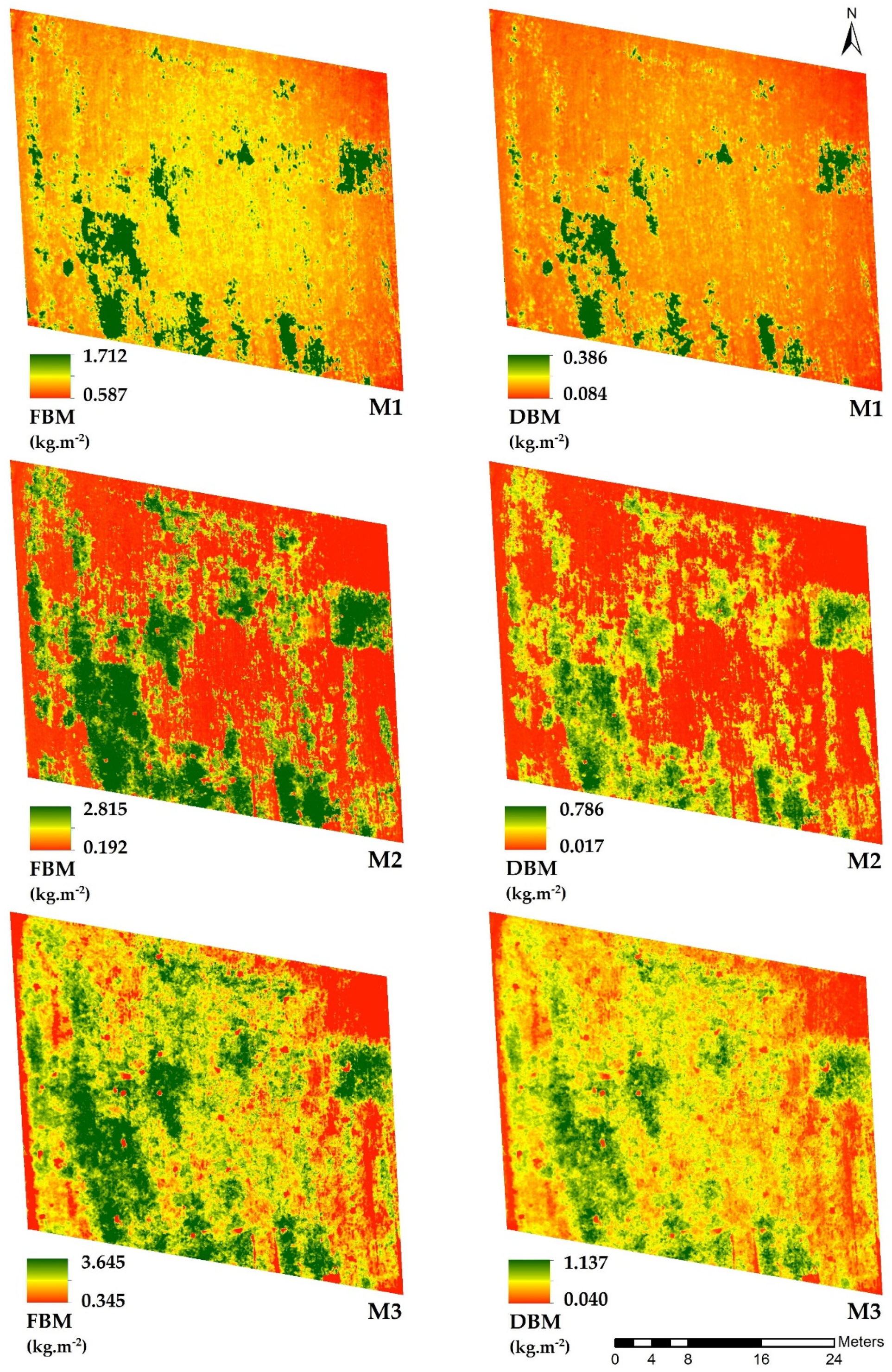
In order to illustrate the spatial and temporal variability of biomass predicted across the test site, several maps were generated estimating FBM and DBM from PHTCSM and calibrated models obtained for different growing stages (Figure 5).
4. Discussion
Considering that plant height usually has a strong correlation with crop biomass [9,15,34], we first assessed the performance of CSMs based on SfM approach to predict plant height. Ground-based PHT reference measurements were compared to PHTCSM resulting in linear regression models with R2 between 0.68 and 0.92. Similar results obtained through SfM algorithms applied to UAV-based imagery were observed for barley (R2 = 0.92) [6], winter wheat (R2 = 0.87–0.96) [1], onion (R2 = 0.82) [30], maize (R2 = 0.88) [29], grassland (R2 = 0.56–0.70) [31] and mixed crops (R2 = 0.80–0.87) [35]. On the other hand, laser scanner approaches based on terrestrial platforms (TLS) achieved R2 values between 0.88 and 0.99 in barley crop [36] and between 0.93 and 0.99 in wheat, oilseed rape and winter rye [37], whereas Li et al. [3] predicted PHT in maize crop with an R2 of 0.79 using an airborne sensor (LiDAR).
During the booting stage (M1) the lowest average plant height measured was observed (0.2 m), which provided the highest relative error (rRMSE) observed (9.6%). As stated by Possoch et al. [10], this limitation must be considered when applied to lower canopies, given that further biomass estimation error might exceed the limits required for practical applications. The highest value of R2 was observed in M2 (R2 = 0.92), where most parts of the plots had plants at the beginning of reproductive stage reaching the highest PHT amplitude and variability between plots (Table 2). This characteristic resulted in a regression model with well-distributed points which contributed to reaching a higher correlation value. On the other hand, the lowest R2 obtained in M3 (R2 = 0.68) can be linked to lodging occurrence. Due to the fertilizer treatments combined to a drought period, some plots had an anticipated senesce and were more likely to lodging. In these plots, the PHT derived from CSMs was lower than non-lodging plots with similar ground-based PHT reducing the performance of the model. A similar condition was observed by Bendig et al. [6] in summer barley, where the inclusion of lodging plots reduced the performance of biomass prediction models, recommending the use of average maximum PHTCSM instead of average mean PHTCSM to mitigate this effect. This observation can also indicate that the number of samples used to determine average PHT as the reference (n = 8) was not sufficient to be compared with PHT obtained from CSMs in situations with high spatial variability across the plot [35]. For each plot sampled (0.25 m²) the CSM-based average PHT was determined based on approximately 700 pixels, which represents more than a pixel per plant. As a consequence, PHT obtained from CSMs tend to be lower in comparison to ground measurements because not only the top portion of the plants are represented in the CSMs, but also the lower parts, like leaves and even the soil level depending on the crop structure, covering more details than ground-based PHT measurements [6].
The regression models for biomass estimation performed differently across the growth stages analyzed, varying according to the results observed in PHT analysis, with best performance during M2 and worst fits in M3, which indicates that biomass modeling is sensible to PHT accuracy. FBM models yielded a coefficient of determination of 0.69-0.94, whereas DBM models achieved an R2 between 0.69 and 0.92. If considered the relative errors of the models (rRMSE), FBM was estimated with errors between 8.9 (M2) and 19.5% (M1), whereas DBM was estimated with errors ranging from 10.5 (M2) to 19.3% (M1). In absolute terms though, M1 yielded the lowest error, with 0.155 kg m−2 for FBM and 0.029 kg m−2 for DBM, while M3 provided the highest residuals, with 0.265 kg m−2 for FBM and 0.071 kg m−2 for DBM. Even though regressions from M1 showed lower absolute residuals, biomass prediction at this growth stage (booting) might not be suitable for practical applications due to higher relative errors. According to Shirmman et al. [1], during early stages biomass is mainly stored in the leaves and not in the stems, resulting in a weaker relationship between PHT and biomass. On the other hand, missions conducted during flowering stage (M2) tend to provide more accurate biomass prediction, with relative errors around 10%. Considering that during M3 plants are more suitable to lodging and PHT growth rate decline with biomass increments due to grain filling, biomass prediction becomes more complex and tend to be erroneous when using only PHT as a dependent variable.
The cross-validation analysis conducted using the entire dataset (M1, M2, M3) aimed to generate robust models, using PHTCSM to predict FBM and DBM across all growth stages analyzed. The calibration step achieved an R2 of 0.64 for FBM and of 0.89 for DBM. Similar results were reported using calibration datasets in barley (FBM-R2 = 0.81, DBM-R2 = 0.82) [6], maize (DBM-R2 = 0.78) [3], onion (DBM-R2 = 0.76) [30], grassland (DBM-R2 = 0.62–0.81) [31] and multiple crops (DBM-R2 = 0.58–0.74) [35]. As stated by Tilly et al. [8], PHT tends to perform better to predict DBM than FBM, especially in multi-temporal analysis, since water content vary accordingly to plant phenology, weather conditions and soil characteristics, adding noise to the FBM prediction model which results in lower R2 values. To evaluate model residuals, we analyzed the results from validation step. FBM was estimated with a relative error of 35.2% which is equal to 0.506 kg m−2, while DBM was predicted with an error of 20.3%, equivalent to 0.063 kg m−2. Comparable results were found using a multi-temporal SfM approach by Grüner et al. [31] in temperate grasslands, achieving relative errors between 16 and 22% for DBM prediction. Another similar study was conducted by Bendig et al. [6], estimating barley biomass with relative errors ranging from 54.04 to 67.72% for FBM and 68.41 to 84.61% for DBM, indicating lower accuracies in biomass estimation. However, several treatments were tested in the experiment, including different cultivars and nitrogen rates, with 18 missions conducted throughout the growing season, as opposed to a single cultivar and three missions carried out in this study.
Compared to studies that estimated biomass from CSMs generated from laser scanner data, UAV-SfM approach tends to provide lower accuracies [6]. These studies reported R2 values of 0.90 for DBM of paddy rice [8], between 0.72 and 0.79 for DBM [38] and 0.91 to 0.95 for FBM [39] in winter wheat and of 0.82 for DBM in maize [3]. Even though laser scanner approaches tend to provide more accurate biomass predictions, most part of these studies rely on TLS data, which is usually suitable for small areas [3]. In contrast, UAVs offer the advantage of a fast, cost-effective and more flexible data acquisition method, and can usually cover larger areas [6]. Apart from methods using PHT, several studies have predicted crop biomass using proximal sensed variables, such as LAI and VIs. Harmoney et al. [40] examined different techniques to predict grassland biomass, including PHT and LAI as predictor variables, concluded that canopy height was more accurate in six of the eight analyzed species. Another study compared point-wise LAI data and PHT derived from UAV imaging in wheat biomass modeling achieved pearson correlation coefficient between 0.82 and 0.98 for LAI and between 0.68 to 0.95 for PHT [1]. Using vegetation indices from visible and near infrared coupled with PHT from CSMs, Bendig et al. [26] tested both VIs and PHT alone as well as combined. None of the VIs tested performed better than PHT alone to predict biomass, although slightly higher R² values were observed when combining PHT with some of the tested VIs. Another approach that uses VIs to model biomass consists of the use of active optical sensors attached to ground-driven vehicles. Erdle et al. [41] evaluated the use of different active optical sensors to monitor biophysical parameters of wheat and achieved R2 values between 0.56 and 0.83 for DBM prediction. Although these proximal sensing methods have a clear potential to model biomass yield, they consist of point-wise data, and require interpolation [1]. In this sense, UAVs images are more feasible and can deliver spatial information with high resolution without interpolation processing.
Moreover, the prediction maps for yield biomass developed using multi-temporal CSMs and the regression models obtained in this study can be useful in spatial variability analysis. Regarding the concept of precision farming, yield maps are considered the starting point to identify spatial variations and to describe their causes [42], which can be linked to soil and weather conditions together with management strategies. Forage production can take advantage of this information to improve yields and quality by means of increased precision in management strategies adopted as well as to make adjustments in the number of animals according to the amount of forage available. The spatial and temporal variability of biomass also can be used to evaluate the performance of cover crops in no-tillage systems by modelling straw yield.
In this study, the SfM approach using RGB-imagery enabled both PHT and biomass modelling for black oats crop with the described uncertainties. The main source of error found was the lodging occurrence, lowering the accuracy of PHT estimation and the biomass prediction. Higher relative errors must be expected when applying this technique in lower canopies, especially during early growth stages, and weaker relationships between PHT and biomass during grain filling. The amount of time required for image acquisition and further processing should also be considered when adopting this method in field-scale, since flight time and processing time increases proportionally to the size of analyzed area. Further evaluations in field-scale and multiple years are important to ensure model robustness and transferability, coupled with more studies focusing on reducing the time necessary for image processing and acquisition and its impact on biomass modelling performance. This is an important step to ensure the method’s feasibility for field conditions, which further studies should evaluate.
5. Conclusions
From UAV-imagery based on an RGB sensor, CSMs were obtained across different growth stages of black oats. The coefficients of determination (R2 = 0.68–0.92) demonstrated a medium-high accuracy in assessing multi-temporal PHT, with best results before senescence (R2 = 0.86–0.92). The multi-temporal CSMs with ultra-high resolution allowed PHT spatial variability detection throughout the missions, covering more details than point-wise ground measurements.
Furthermore, we investigated the relationship between PHT derived from CSMs and crop biomass. Several models to estimate FBM and DBM at different growth stages were developed, explaining 69–94% of biomass variability. In addition, two models were built using observations from all missions, with calibration and validation steps. The results showed that PHT is highly correlated with DBM and medium correlated with FBM, estimating biomass with an rRMSE of 20.3% and 35.2%, respectively.
Based on multi-temporal CSMs and the models developed in this study, yield maps were built illustrating spatial and temporal variability of FBM and DBM. This information expresses spatial patterns that might be connected with environmental factors, such as soil heterogeneity, and can be further used to optimize the crop management following PA concepts.
Author Contributions
M.G.A., F.d.D.A.M. and M.M. conceived the idea, M.G.A., L.R.S. and D.A.S. designed and performed the experiment, M.G.A. and M.M. analyzed the data, and all authors contributed to the writing of the manuscript.
Acknowledgments
The authors would like to thank the Federal Technological University of Paraná staff for supporting this research project, providing the land as experimental field and for seeding, raising and taking care of the crops.
Conflicts of Interest
The authors declare no conflict of interest.
References
- Schirrmann, M.; Giebel, A.; Gleiniger, F.; Pflanz, M.; Lentschke, J.; Dammer, K.-H. Monitoring Agronomic Parameters of Winter Wheat Crops with Low-Cost UAV Imagery. Remote Sens. 2016, 8, 706. [Google Scholar] [CrossRef]
- Thorp, K.R.; Wang, G.; West, A.L.; Moran, M.S.; Bronson, K.F.; White, J.W.; Mon, J. Estimating crop biophysical properties from remote sensing data by inverting linked radiative transfer and ecophysiological models. Remote Sens. Environ. 2012, 124, 224–233. [Google Scholar] [CrossRef] [Green Version]
- Li, W.; Niu, Z.; Huang, N.; Wang, C.; Gao, S.; Wu, C. Airborne lidar technique for estimating biomass components of maize: A case study in Zhangye City, Northwest China. Ecol. Indic. 2015, 57, 486–496. [Google Scholar] [CrossRef]
- Fischer, R.A. Irrigated spring wheat and timing and amount of nitrogen fertilizer. II. Physiology of grain yield response. Field Crops Res. 1993, 33, 57–80. [Google Scholar] [CrossRef]
- Boukerrou, L.; Rasmusson, D.D. Breeding for high biomass yield in Spring Barley. Crop Sci. 1990, 30, 31–35. [Google Scholar] [CrossRef]
- Bendig, J.; Bolten, A.; Bennertz, S.; Broscheit, J.; Eichfuss, S.; Bareth, G. Estimating Biomass of Barley Using Crop Surface Models (CSMs) Derived from UAV-Based RGB Imaging. Remote Sens. 2014, 6, 10395–10412. [Google Scholar] [CrossRef] [Green Version]
- Chen, P.; Haboudane, D.; Tremblay, N.; Wang, J.; Vigneault, P.; Li, B. New spectral indicator assessing the efficiency of crop nitrogen treatment in corn and wheat. Remote Sens. Environ. 2010, 114, 1987–1997. [Google Scholar] [CrossRef]
- Tilly, N.; Hoffmeister, D.; Cao, Q.; Huang, S.; Lenz-Wiedemann, V.I.S.; Miao, Y.; Bareth, G. Multitemporal crop surface models: Accurate plant height measurement and biomass estimation with terrestrial laser scanning in paddy rice. J. Appl. Remote Sens. 2014, 8, 83671. [Google Scholar] [CrossRef]
- Prost, L.; Jeuffroy, M.-H. Replacing the nitrogen nutrition index by the chlorophyll meter to assess wheat N status. Agron. Sust. Dev. 2007, 27, 321–330. [Google Scholar] [CrossRef] [Green Version]
- Possoch, M.; Bieker, S.; Hoffmeister, D.; Bolten, A.; Schellberg, J.; Bareth, G. Multi-temporal crop surface models combined with the RGB vegetation index from UAV-based images for forage monitoring in grassland. Int. Arch. Photogram. Rem. Sens. Spat. Inform. Sci. 2016, XLI-B1, 991–998. [Google Scholar] [CrossRef]
- Cargnelutti Filho, A.; Toebe, M.; Alves, B.M.; Burin, C.; dos Santos, G.O.; Facco, G.; Neu, I.M.M. Linear relations among characters of black oat. Ciênc Rural 2015, 45, 985–992. [Google Scholar] [CrossRef]
- Kliemann, H.J.; Braz, A.J.P.B.; Silveira, P.M. Taxas de decomposição de resíduos de espécies de cobertura em latossolo vermelho distroférrico. Rev. Agropec. Trop. 2006, 36, 21–28. Available online: https://www.revistas.ufg.br/pat/article/view/2165/2116 (accessed on 15 January 2019).
- Calvo, C.L.; Foloni, J.S.S.; Brancalião, S.R. Produtividade de fitomassa e relação C/N de monocultivo e consórcios de guandu-anão, milheto e sorgo em três épocas de corte. Bragantia. 2010, 69, 77–86. [Google Scholar] [CrossRef]
- Lumme, J.; Karjalainen, M.; Kaartinen, H.; Kukko, A.; Hyyppä, J.; Hyyppä, H.; Jaakkola, A.; Kleemola, J. Terrestrial laser scanning of agricultural crops. Int. Arch. Photogramm. Remote Sens. Spat. Inf. Sci. 2008, 37, 563–566. Available online: https://pdfs.semanticscholar.org/6c45/b5f5481125a311ea46a05e7acfa1de0f2cfb.pdf (accessed on 15 January 2019).
- Hakl, J.; Hrevušová, Z.; Hejcman, M.; Fuksa, P. The use of a rising plate meter to evaluate lucerne (Medicago sativa L.) height as an important agronomic trait enabling yield estimation. Grass Forage Sci. 2012, 67, 589–596. [Google Scholar] [CrossRef]
- Breda, N.J.J. Ground-based measurements of leaf area index: A review of methods, instruments and current controversies. J. Exp. Bot. 2003, 54, 2403–2417. [Google Scholar] [CrossRef] [PubMed]
- Ahamed, T.; Tian, L.; Zhang, Y.; Ting, K.C. A review of remote sensing methods for biomass feedstock production. Biomass Bioenergy 2011, 35, 2455–2469. [Google Scholar] [CrossRef]
- Marshall, M.; Thenkabail, P. Developing in situ Non-destructive estimates of crop biomass to address issues of scale in Remote Sensing. Remote Sens. 2015, 7, 808–835. [Google Scholar] [CrossRef]
- Moeckel, T.; Safari, H.; Reddersen, B.; Fricke, T.; Wachendorf, M. Fusion of Ultrasonic and Spectral Sensor Data for Improving the Estimation of Biomass in Grasslands with Heterogeneous Sward Structure. Remote Sens. 2017, 9, 98. [Google Scholar] [CrossRef]
- Cao, Q.; Cui, Z.; Chen, X.; Khosla, R.; Dao, T.H.; Miao, Y. Quantifying spatial variability of indigenous nitrogen supply for precision nitrogen management in small scale farming. Precis. Agric. 2012, 13, 45–61. [Google Scholar] [CrossRef]
- Höfle, B. Radiometric correction of terrestrial LiDAR point cloud data for individual maize plant detection. IEEE Geosci. Remote Sens. Lett. 2014, 1, 94–98. [Google Scholar] [CrossRef]
- Bendig, J.V. Unmanned aerial vehicles (UAVs) for multi-temporal crop surface modelling—A new method for plant height and biomass estimation based on RGB-imaging. Ph.D. Thesis, University of Cologne, Cologne, Germany, 12 January 2014. Available online: https://kups.ub.uni-koeln.de/6018 (accessed on 15 January 2019).
- Berni, J.A.J.; Zarco-Tejada, P.J.; Suárez, L.; Fereres, E. Thermal and narrowband multispectral remote sensing for vegetation monitoring from an unmanned aerial vehicle. IEEE Trans. Geosci. Remote Sens. 2009, 47, 722–738. [Google Scholar] [CrossRef]
- Colomina, I.; Molina, P. Unmanned aerial systems for photogrammetry and remote sensing: A review. ISPRS J. Photogramm. Remote Sens. 2014, 92, 79–97. [Google Scholar] [CrossRef] [Green Version]
- Swain, K.C.; Zaman, Q.U. Rice crop monitoring with unmanned helicopter remote sensing images. In Remote Sensing of Biomass—Principles and Applications; Fatoyinbo, L., Ed.; INTECH Open Access Publisher: Rijeka, Croatia, 2012; pp. 253–272. [Google Scholar]
- Bendig, J.; Yu, K.; Aasen, H.; Bolten, A.; Bennertz, S.; Broscheit, J.; Gnyp, M.L.; Bareth, G. Combining UAV-based plant height from crop surface models, visible, and near infrared vegetation indices for biomass monitoring in barley. Int. J. Appl. Earth Obs. Geoinf. 2015, 39, 79–87. [Google Scholar] [CrossRef]
- Verhoeven, G. Taking computer vision aloft—Archaeological three-dimensional reconstructions from aerial photographs with photoscan. Archaeol. Prospect. 2011, 18, 67–73. [Google Scholar] [CrossRef]
- Hoffmeister, D.; Bolten, A.; Curdt, C.; Waldhoff, G.; Bareth, G. High resolution Crop Surface Models (CSM) and Crop Volume Models (CVM) on field level by terrestrial laser scanning. Proc. SPIE 2010, 7840. [Google Scholar] [CrossRef]
- Li, W.; Niu, Z.; Chen, H.; Li, D.; Wu, M.; Zhao, W. Remote estimation of canopy height and aboveground biomass of maize using high-resolution stereo images from a low-cost unmanned aerial vehicle system. Ecol. Indic. 2016, 67, 637–648. [Google Scholar] [CrossRef]
- Ballesteros, R.; Ortega, J.F.; Hernandez, D.; Moreno, M.A. Onion biomass monitoring using UAV-based RGB imaging. Precis. Agric. 2018, 19, 840–857. [Google Scholar] [CrossRef]
- Grüner, E.; Astor, T.; Wachendorf, M. Biomass Prediction of Heterogeneous Temperate Grasslands Using an SfM Approach Based on UAV Imaging. Agronomy 2019, 9, 54. [Google Scholar] [CrossRef]
- Cooper, S.; Roy, D.; Schaaf, C.; Paynter, I. Examination of the Potential of Terrestrial Laser Scanning and Structure-from-Motion Photogrammetry for Rapid Nondestructive Field Measurement of Grass Biomass. Remote Sens. 2017, 9, 531. [Google Scholar] [CrossRef]
- Alvares, C.A.; Stape, J.L.; Sentelhas, P.C.; de Moraes Gonçalves, J.L.; Sparovek, G. Köppen’s climate classification map for Brazil. Meteorol. Z. 2013, 22, 711–728. [Google Scholar] [CrossRef]
- Scotford, I.M.; Miller, P.C.H. Combination of spectral reflectance and ultrasonic sensing to monitor the growth of winter wheat. Biosyst. Eng. 2004, 87, 27–38. [Google Scholar] [CrossRef]
- Roth, L.; Streit, B. Predicting cover crop biomass by lightweight UAS-based RGB and NIR photography: An applied photogrammetric approach. Precis. Agric. 2018, 19, 93–114. [Google Scholar] [CrossRef]
- Tilly, N.; Aasen, H.; Bareth, G. Fusion of plant height and vegetation indices for the estimation of barley biomass. Remote Sens. 2015, 7, 11449–11480. [Google Scholar] [CrossRef]
- Ehlert, D.; Horn, H.-J.; Adamek, R. Measuring crop biomass density by laser triangulation. Comput. Electron. Agric. 2008, 61, 117–125. [Google Scholar] [CrossRef]
- Eitel, J.U.H.; Magney, T.S.; Vierling, L.A.; Brown, T.T.; Huggins, D.R. LiDAR based biomass and crop nitrogen estimates for rapid, non-destructive assessment of wheat nitrogen status. Field Crop Res. 2014, 159, 21–32. [Google Scholar] [CrossRef]
- Ehlert, D.; Heisig, M.; Adamek, R. Suitability of a laser rangefinder to characterize winter wheat. Precis. Agric. 2010, 11, 650–663. [Google Scholar] [CrossRef]
- Harmoney, K.R.; Moore, K.J.; George, J.R.; Brummer, E.C.; Russell, J.R. Determination of pasture biomass using four indirect methods. Agron. J. 1997, 89, 665–672. [Google Scholar] [CrossRef]
- Erdle, K.; Mistele, B.; Schmidhalter, U. Comparison of active and passive spectral sensors in discriminating biomass parameters and nitrogen status in wheat cultivars. Field Crop Res. 2011, 124, 74–84. [Google Scholar] [CrossRef]
- Khosla, R.; Westfall, D.G.; Reich, R.M.; Mahal, J.S.; Gangloff, W.J. Spatial Variation and Site-Specific Management Zones. In Geostatistical Applications for Precision Agriculture; Oliver, M.A., Ed.; Springer Science: Berlin, Germany, 2010; pp. 195–219. [Google Scholar]
Figure 1.
Procedure to extract plot-wise variables from UAV-based dataset. (a) Orthomosaic built from images collected after sampling procedure; (b) Mask created for the sampled area; (c) Extraction of CSM data using generated masks.
Figure 1.
Procedure to extract plot-wise variables from UAV-based dataset. (a) Orthomosaic built from images collected after sampling procedure; (b) Mask created for the sampled area; (c) Extraction of CSM data using generated masks.
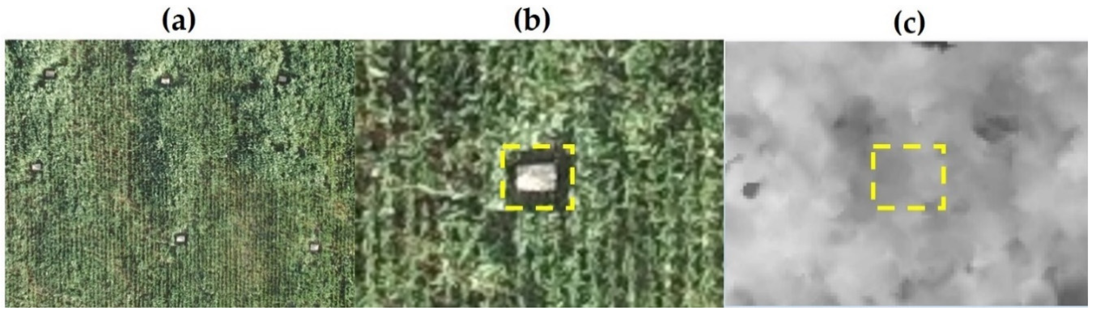
Figure 2.
Linear regression between plant height deviated from CSM (PHTCSM) and manual height measurements (PHTref) for each mission. p < 0.001 for all R2. Symbols indicate datasets from Mission 1 (●), Mission 2 (▲), and Mission 3 (∎).
Figure 2.
Linear regression between plant height deviated from CSM (PHTCSM) and manual height measurements (PHTref) for each mission. p < 0.001 for all R2. Symbols indicate datasets from Mission 1 (●), Mission 2 (▲), and Mission 3 (∎).
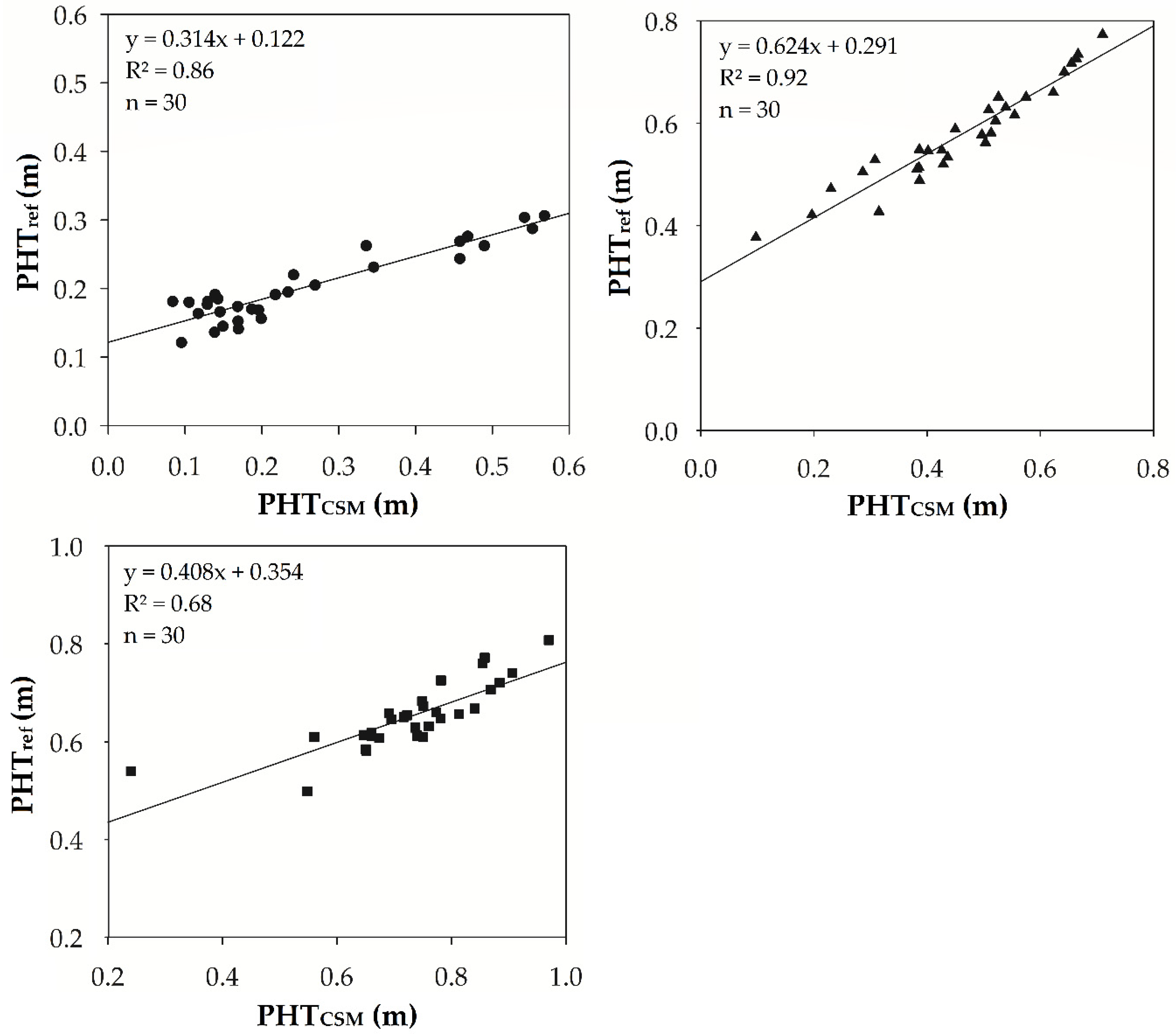
Figure 3.
Regression models between FBM/DBM and PHTCSM for each mission. p < 0.001 for all R2. Symbols indicate datasets from Mission 1 (●), Mission 2 (▲), and Mission 3 (∎).
Figure 3.
Regression models between FBM/DBM and PHTCSM for each mission. p < 0.001 for all R2. Symbols indicate datasets from Mission 1 (●), Mission 2 (▲), and Mission 3 (∎).
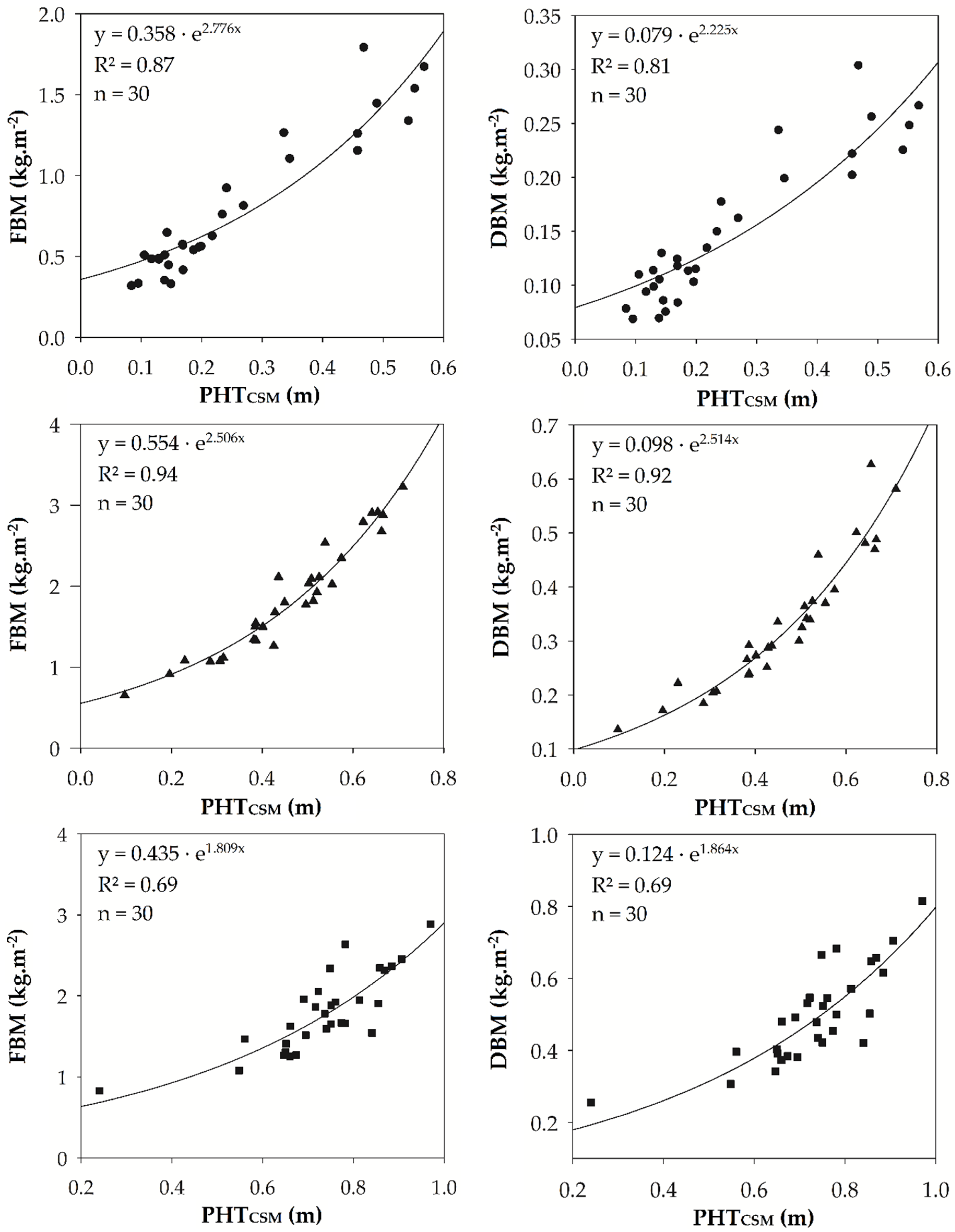
Figure 4.
Cross-validation relationship between biomass and PHTCSM for FBM (a) and DBM (b) from calibration datasets and between observed versus predicted FBM (c) and DBM (d) derived from validation dataset. Symbols indicate datasets from Mission 1 (●), Mission 2 (▲), and Mission 3 (∎).
Figure 4.
Cross-validation relationship between biomass and PHTCSM for FBM (a) and DBM (b) from calibration datasets and between observed versus predicted FBM (c) and DBM (d) derived from validation dataset. Symbols indicate datasets from Mission 1 (●), Mission 2 (▲), and Mission 3 (∎).

Figure 5.
Prediction maps for FBM and DBM of each mission derived from CSMs using calibrated models (Table 4). M1 = Mission 1; M2 = Mission 2; M3 = Mission 3.
Figure 5.
Prediction maps for FBM and DBM of each mission derived from CSMs using calibrated models (Table 4). M1 = Mission 1; M2 = Mission 2; M3 = Mission 3.

Table 1.
Flight mission details. ID = mission number; DTM = digital terrain model; DSM = digital surface model; DAS = days after sowing; GSD = ground sample distance.
Table 1.
Flight mission details. ID = mission number; DTM = digital terrain model; DSM = digital surface model; DAS = days after sowing; GSD = ground sample distance.
| ID | Date | Mission Objective | Growth Stage (DAS) | Wind Speed 1 | Images Collected | Point Density (pt·m−2) | Image Overlap 2 | GSD (cm·px−1) |
|---|---|---|---|---|---|---|---|---|
| M0 | 4 June 2017 | DTM | - | 1.1 | 150 | 3228 | >9 | 1.76 |
| M1 | 11 August 2017 | DSM | Booting (53) | 4.1 | 142 | 2916 | >9 | 1.85 |
| M2 | 25 August 2017 | DSM | Flowering (67) | 3.4 | 179 | 4056 | >9 | 1.57 |
| M3 | 6 September 2017 | DSM | Grain filling (79) | 3.3 | 153 | 3052 | >9 | 1.81 |
1 Averaged wind speed considering wind gusts. 2 Number of images covering the same part of the experimental field.
Table 2.
Descriptive statistics of the crop parameters measured at the sample plots for M1, M2, and M3. n = number of samples; SD = standard deviation.
Table 2.
Descriptive statistics of the crop parameters measured at the sample plots for M1, M2, and M3. n = number of samples; SD = standard deviation.
| Variable | n | Unit | Abbreviation | Mean | Min | Max | SD | Median | |
|---|---|---|---|---|---|---|---|---|---|
| Mission 1 | Reference plant height | 30 | m | PHTref | 0.20 | 0.12 | 0.31 | 0.05 | 0.18 |
| CSM plant height | 30 | m | PHTCSM | 0.25 | 0.08 | 0.57 | 0.15 | 0.19 | |
| Fresh Biomass | 30 | kg·m−2 | FBM | 0.795 | 0.320 | 1.793 | 0.440 | 0.573 | |
| Dry Biomass | 30 | kg·m−2 | DBM | 0.149 | 0.069 | 0.304 | 0.068 | 0.121 | |
| Mission 2 | Reference plant height | 30 | m | PHTref | 0.58 | 0.38 | 0.77 | 0.10 | 0.57 |
| CSM plant height | 30 | m | PHTCSM | 0.46 | 0.10 | 0.71 | 0.15 | 0.47 | |
| Fresh Biomass | 30 | kg·m−2 | FBM | 1.869 | 0.655 | 3.230 | 0.685 | 1.811 | |
| Dry Biomass | 30 | kg·m−2 | DBM | 0.334 | 0.136 | 0.627 | 0.123 | 0.313 | |
| Mission 3 | Reference plant height | 30 | m | PHTref | 0.65 | 0.50 | 0.81 | 0.07 | 0.65 |
| CSM plant height | 30 | m | PHTCSM | 0.73 | 0.24 | 0.97 | 0.14 | 0.74 | |
| Fresh Biomass | 30 | kg·m−2 | FBM | 1.794 | 0.829 | 2.885 | 0.482 | 1.723 | |
| Dry Biomass | 30 | kg·m−2 | DBM | 0.497 | 0.255 | 0.815 | 0.130 | 0.486 |
Table 3.
Regression models obtained between plant height and biomass for different missions and its residuals. x = dependent variable; y = independent variable; ME = mean error; MAE = mean absolute error; RMSE = root mean square error; rRMSE = relative RMSE; p < 0.001 for all R².
Table 3.
Regression models obtained between plant height and biomass for different missions and its residuals. x = dependent variable; y = independent variable; ME = mean error; MAE = mean absolute error; RMSE = root mean square error; rRMSE = relative RMSE; p < 0.001 for all R².
| Y | x | Model | n | R2 | ME | MAE | RMSE | rRMSE | |
|---|---|---|---|---|---|---|---|---|---|
| Mission 1 | PHTref | PHTCSM | 0.314x + 0.122 | 30 | 0.86 | 0.000 | 0.016 | 0.019 | 9.6 |
| FBM | PHTCSM | 0.358 · exp(2.776x) | 30 | 0.87 | 0.005 | 0.111 | 0.155 | 19.5 | |
| DBM | PHTCSM | 0.079 · exp(2.255x) | 30 | 0.81 | 0.000 | 0.022 | 0.029 | 19.3 | |
| Mission 2 | PHTref | PHTCSM | 0.624 x + 0.291 | 30 | 0.92 | 0.000 | 0.024 | 0.028 | 4.8 |
| FBM | PHTCSM | 0.554 · exp(2.506x) | 30 | 0.94 | 0.003 | 0.126 | 0.165 | 8.9 | |
| DBM | PHTCSM | 0.098 · exp(2.514x) | 30 | 0.92 | -0.002 | 0.025 | 0.035 | 10.5 | |
| Mission 3 | PHTref | PHTCSM | 0.408x + 0.354 | 30 | 0.68 | 0.000 | 0.030 | 0.037 | 5.7 |
| FBM | PHTCSM | 0.435 · exp(1.899x) | 30 | 0.69 | 0.001 | 0.208 | 0.265 | 14.8 | |
| DBM | PHTCSM | 0.124 · exp(1.864x) | 30 | 0.69 | 0.001 | 0.058 | 0.071 | 14.3 |
Table 4.
Cross-validation results between fresh/dry biomass and PHTCSM for all missions. x = dependent variable; y = independent variable; ME = mean error; MAE = mean absolute error; RMSE = root mean square error; rRMSE = relative RMSE; p < 0.001 for all R2.
Table 4.
Cross-validation results between fresh/dry biomass and PHTCSM for all missions. x = dependent variable; y = independent variable; ME = mean error; MAE = mean absolute error; RMSE = root mean square error; rRMSE = relative RMSE; p < 0.001 for all R2.
| y | x | Model | n | R² | ME | MAE | RMSE | rRMSE | |
|---|---|---|---|---|---|---|---|---|---|
| Cal. | FBM | PHTCSM | 0.707 · exp(1.438x) | 63 | 0.64 | 0.013 | 0.354 | 0.438 | 29.1 |
| DBM | PHTCSM | 0.109 · exp(2.056x) | 63 | 0.89 | 0.004 | 0.048 | 0.064 | 19.1 | |
| Val. | FBM | PHTCSM | 1.206x − 0.3220 | 27 | 0.52 | 0.020 | 0.394 | 0.506 | 35.2 |
| DBM | PHTCSM | 1.086x − 0.0335 | 27 | 0.84 | 0.006 | 0.052 | 0.063 | 20.3 |
© 2019 by the authors. Licensee MDPI, Basel, Switzerland. This article is an open access article distributed under the terms and conditions of the Creative Commons Attribution (CC BY) license (http://creativecommons.org/licenses/by/4.0/).
Share and Cite
MDPI and ACS Style
Acorsi, M.G.; das Dores Abati Miranda, F.; Martello, M.; Smaniotto, D.A.; Sartor, L.R. Estimating Biomass of Black Oat Using UAV-Based RGB Imaging. Agronomy 2019, 9, 344. https://doi.org/10.3390/agronomy9070344
AMA Style
Acorsi MG, das Dores Abati Miranda F, Martello M, Smaniotto DA, Sartor LR. Estimating Biomass of Black Oat Using UAV-Based RGB Imaging. Agronomy. 2019; 9(7):344. https://doi.org/10.3390/agronomy9070344
Chicago/Turabian StyleAcorsi, Matheus Gabriel, Fabiani das Dores Abati Miranda, Maurício Martello, Danrley Antonio Smaniotto, and Laercio Ricardo Sartor. 2019. "Estimating Biomass of Black Oat Using UAV-Based RGB Imaging" Agronomy 9, no. 7: 344. https://doi.org/10.3390/agronomy9070344
Note that from the first issue of 2016, this journal uses article numbers instead of page numbers. See further details here.