Climate Variability and Its Impact on Forest Hydrology on South Carolina Coastal Plain, USA

 ,
,
Abstract
: Understanding the changes in hydrology of coastal forested wetlands induced by climate change is fundamental for developing strategies to sustain their functions and services. This study examined 60 years of climatic observations and 30 years of hydrological data, collected at the Santee Experimental Forest (SEF) in coastal South Carolina. We also applied a physically-based, distributed hydrological model (MIKE SHE) to better understand the hydrological responses to the observed climate variability. The results from both observation and simulation for the paired forested watershed systems indicated that the forest hydrology was highly susceptible to change due to climate change. The stream flow and water table depth was substantially altered with a change in precipitation. Both flow and water table level decreased with a rise in temperature. The results also showed that hurricanes substantially influenced the forest hydrological patterns for a short time period (several years) as a result of forest damage.1. Introduction
Hydrological response to climate change has been widely recognized [1–7]. The climate change is not only about rising surface air temperature [8], but also about altering precipitation patterns [9–11], leading to changes in hydrologic cycles at multiple scales [12,13]. Because there are substantial differences in global climate change in space, such as the differences between ocean and land, and between lower and higher latitudes [8], the change can bring different consequences to different areas. For example, global warming can bring more rain to middle and high latitude zones, but not to low latitude areas [11]. Therefore, the hydrologic response to these changes may vary from region to region [6,14–16].
The impact of global warming on wetland hydrology has been studied [17–21], especially with respect to coastal wetlands [20,22,23]. Most studies on the impact of global warming on coastal wetlands are concentrated on wetland's loss to sea level rise. However, climate change can also cause changes in the function and services of coastal wetlands through altering their hydrologic characteristics [19,24]. For example, some wetlands may not be lost to sea level rise, but their salinity is likely changed due to global sea level rise leading to a salt water intrusion [23]. Some freshwater wetlands may lose to a decrease in fresh water inputs rather than to sea level rise, especially in middle and low latitude zones due to global warming-induced hydrologic drought [11]. Consequently, the functions and services of these wetland ecosystems are inevitably affected by climate change [25–28]. Therefore, understanding the hydrologic response of coastal wetlands to global warming/climate change is needed to assess ramifications of climate change to coastal wetland ecosystems, especially to those ecosystems in middle and low latitude areas where rainfall is expected to decrease.
Many scientists believe that global warming will increase the frequency and/or intensity of tropical storms due to an increase of sea surface temperature [29–33]. Strong storms (Category 3, 4 and 5) can destroy forests impacting their hydrologic regime. The impact of hurricanes on hydrology has been widely studied [34–38]. Most of those studies on the impact of hurricane on hydrology and nutrient exports were concentrated on the direct and short-term implications caused by flooding and/or strong wind [39,40]. However, hurricanes may cause longer term changes to forest hydrology due to changes in forest composition, which can lead to a change in evapotranspiration. Therefore, long-term hydrologic and climatic observations following a hurricane impact may be very useful to understand the long-term impact of hurricanes on forest hydrology in coastal areas.
The hydrology of forested wetland watersheds on Atlantic Coastal Plain in the Carolinas, especially of the first-order watersheds, is heavily dependent on precipitation and evapotranspiration [12,26,41–43]. Those first and second, even third order watersheds can lose their flow in normal dry periods, and regain them in wet periods [13,44,45]. On the contrary, storms leading to flooding problems are not uncommon on the coastal plain [43,46–50]. The water table in those first-order forested watersheds can substantially decrease with a decrease in precipitation and an increase in temperature [41,51,52] because the annual evapotranspiration (ET) is approximate to potential ET (PET) in this area [41,53–55]. These alterations of ET due to climate change suggest that the effect will also be on the water balance and thus stream flow and water table [12,17,22,23,26,51]. The objective of this study is to (1) examine the stream flow and water table dynamics between 1950 and 2007 for a second-order coastal forested watershed on the Santee Experimental Forest using a distributed hydrological model MIKE SHE [56] calibrated and validated against long-term hydrological observations (1964–2007) and (2) assess the impacts of climate variability and Hurricane Hugo on the hydrology of the forested watersheds on the Santee Experimental Forest using long-term climatic (1946–2007) and hydrological (1964–2007) measurements and hydrological simulations (1950–2007). MIKE SHE is widely used for modeling watershed scale hydrology around the world [51,57–59], and has been tested and determined to be suitable for simulating the hydrology for a sub-watershed of the subject watershed of this study [45].
2. Materials and Methods
2.1. Study Site
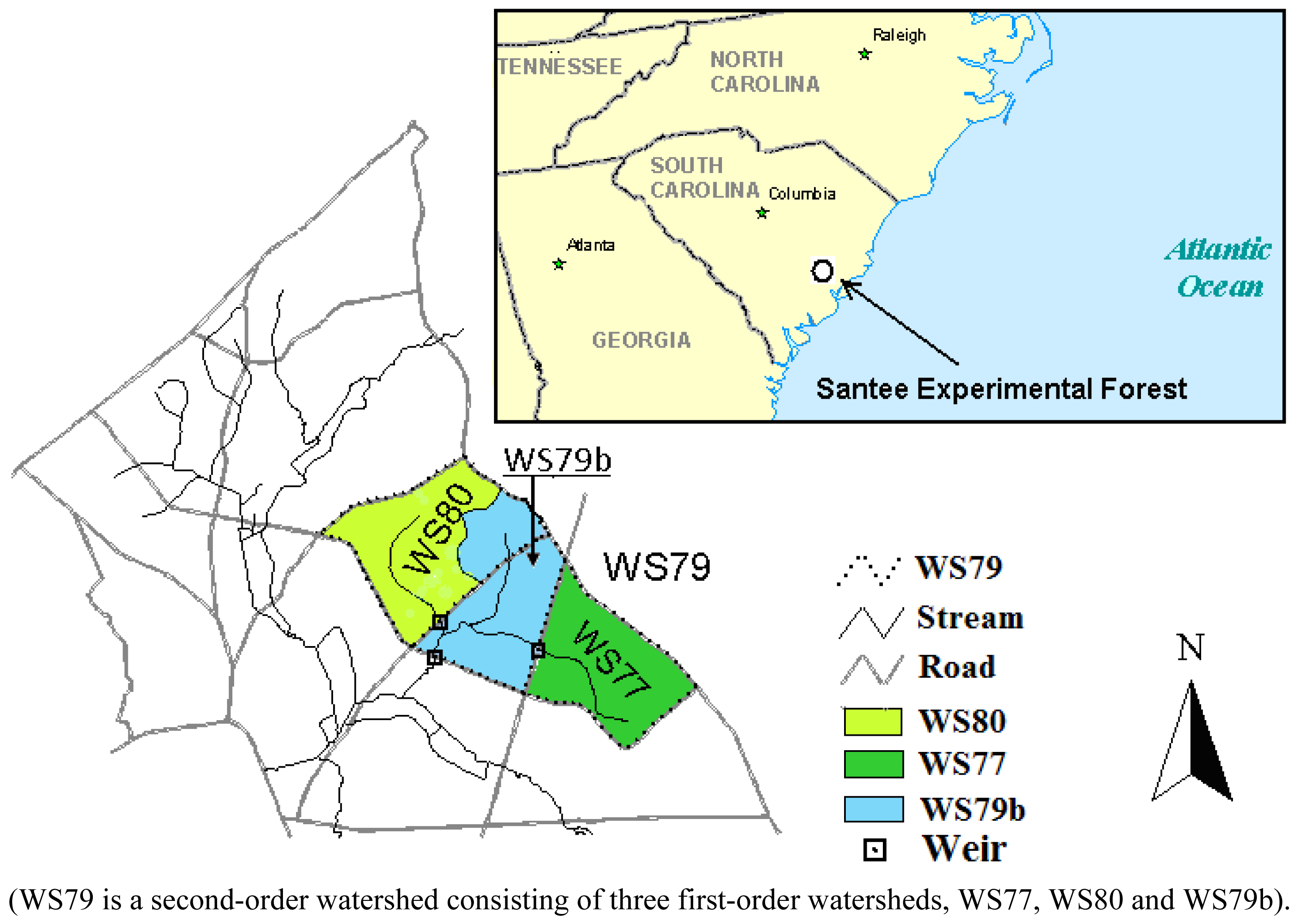
The Santee Experimental Forest (SEF) is located at 33.15° N and 79.8° W, within the Francis Marion National Forest, about 55 km northwest of Charleston, in Berkeley County, South Carolina, USA (Figure 1). The SEF was established in 1937 for scientific research on forests and water in a coastal plain setting [60]. The watershed WS79 was created in 1963. The drainage area is 500 ha consisting of three first-order watersheds, WS77, WS80 and the WS79b which is the part between WS77 and WS80 (Figure 1). WS77 and WS80 serve as a paired watershed system, with WS77 as a treatment catchment, WS80 as a control and WS79b as a mixed watershed with control and treatment. WS80 has not been actively managed over five decades. This paired system is being used for studies on watershed hydrology, biogeochemistry and forest managements including prescribed fire and thinning, and effects of global/environmental changes on forest ecosystems in last three decades.
This site is characteristic of the subtropical region of the Atlantic Coast with long and hot summers, and short, warm and humid winters. The long-term annual average temperature (1946–2007) is 18.5 °C, and averaged annual precipitation is 1370 mm in the same period. The extremely high temperature (over 40 °C) can occur in summers, such as 40.5 °C occurred on June 26 of 1952 and July 21 of 1977, and the extremely low temperature (lower than −14 °C) occurred on January 21 of 1985 in the last 60 years.
The SEF was an agricultural wetland area (rice paddy) in history [61–63], and converted to a forestland in 19th century. The earlier trees were clearly cut in earlier 20th century [62,63], and regenerated afterwards. However, Hurricane Hugo, which was a Category 4 storm, passed through the Francis Marion National Forest area in September of 1989, over 80% of dominant trees were, broken or uprooted [40,64,65]. After the hurricane, the control watershed WS80 remained unmanaged, without biomass removal or salvage logging [45,55,66]. However, most fallen trees were removed from other watersheds, including WS77 and WS79b. The current vegetation coverage regenerated after the hurricane with mostly bottomland hardwoods in riparian zone, pine in uplands, and mixed pine-hardwoods elsewhere. The dominant trees are loblolly (Pinus taeda L.), sweetgum (Liquidambar styraciflua) and a variety of oak species (Quercus spp.) in both the uplands and bottomlands, which is typical of the Atlantic Coastal Plain [64,66]. However, the vegetation coverage in WS77 contains more pine than WS80 and WS79b. In recent years, some artificial disturbances, including prescribed fire and thinning of the forest were installed on WS77 and the treatment part of WS79b for understanding the impacts of these perturbations on the forest and water. As a result, the biomass in the treatment areas has been lowered to some extent, especially with respect to the understory layer and forest floor on the treatment plots. Details of the chronological sequence of activities on these watersheds until 2005 have been reported [60].
The soils, developed in coastal plain sediments, are hydric [67,68], and drained moderately well in the upland and poorly in the riparian zones [69]. The main soil type is loam, covering about 90% of the watershed. Clay content is ≤ 30% in topsoil (within 30 cm), 40–60% in subsoil (>30 cm) [69]. Soil reaction is acidic; pH is between 4.5 and 6.5. Details of the soil hydraulic properties of the watersheds have been reported [66,69].
2.2. Data Collections and Field Measurements
Daily precipitation and daily minimum and maximum temperature were measured manually at the weather station at the Santee Experimental Forest Headquarters (SHQ) between 1946 and 1995 and using an automatic Campbell Scientific weather station afterwards; air and soil temperature, relative humidity, wind speed, wind direction, vapor pressure, solar and net radiation were measured at 30-minute intervals beginning in 2003. Three onsite weather stations (Met 5 on WS77, Lotti adjacent to WS79b and Met25 on WS80) started to manually record daily precipitation and temperature from 1963, 1971 and 1990, respectively, to 2001, and automatically collect data at hourly intervals since 2003. Although the climate data from these stations were comparable, there were some differences in summer precipitation, especially during storms. However, some of the precipitation and temperature data were found to be missing at different stations and/or in different time periods before 2003 due to equipment failure for some time and natural disasters such as Hurricane Hugo in 1989. The missing temperature data for SHQ were at first established by using the regression equations developed from the measurements of daily maximum and minimum temperature between 1972 and 2001 at SHQ and Lotti (about 3 km away from SHQ); and then the remaining missing temperature for SHQ were established by using the regression equations developed from the measurements between 1950 and 2008 at SHQ and Charleston International Airport (CHS, about 50 km away from the SHQ), and the observations between 1996 and 2008 at the SHQ and Moncks Corner (MC, about 20 km away). The missing precipitation data were filled based on evaluation of precipitation measurements from 15 weather stations around SHQ. We assumed that there was no precipitation at SHQ if precipitation was found only at one side of SHQ, otherwise the precipitation at SHQ was the same as the precipitation at the nearest weather station or the average from the weather stations at both sides of SHQ.
The stream stage heights above V-notch weirs were recorded since 1963, 1966 and 1968, for WS77, WS79 and WS80, respectively. The flow rate was calculated in cubic meters per second (cms) using standard rating curve methods developed for these weirs, and then integrated into daily, monthly and annual values after normalizing from cms to millimeters per day by dividing the watershed area to be comparable to daily precipitation. However, the flow data were missing for several periods due to equipment failures, and remained missing, including in calculation of daily, monthly and annual values.
Runoff coefficients (ROC) for monthly and annual periods were calculated by dividing the stream flow by precipitation. Precipitation was used for WS77 from the on-site gauge Met 5, but the precipitation data used for WS80 before 1990 was from SHQ.
Distributed water table depth on WS77 was observed biweekly by using twenty four manual wells installed across the watershed for the time period from 1964 to 1971 and measured weekly by using forty two manual wells from 1992 to 1994, respectively. Thirty three manual wells were installed across WS80 to weekly measure the water table depth between 1992 and 1994. Two automatic recording wells were separately installed on WS77 and WS80 to measure water table depth at 4-hour intervals after 2002. The water table depth was integrated into monthly and annual values. Some details with respect to the instrument and measurement installations were reported by Amatya and Trettin [60].
2.3. MIKE SHE Model Setup and Parameterization
MIKE SHE [56,70,71] is a distributed hydrological modeling system well designed and validated for the applications in low-relief terrains. The model and its algorithms have been described in many publications [56-58,70,71]. In this study, MIKE SHE was coupled with the flow routing model MIKE 11 [56,58], a one-dimensional river/channel water movement model, to simulate the full hydrological cycle of the watershed, including evapotranspiration, infiltration, unsaturated flow, saturated flow, overland flow and stream flow. The main inputs for the model include spatial data on topography, soils, vegetation, and drainage network; and temporal data on daily precipitation and potential evapotranspiration (PET).
Daily PET was estimated using standard Penman-Monteith (P-M) equation for a grass reference for the time period from 2003–2008 [72,73] and Hargreaves equation for the entire period from 1950–2008 [74] because the observations for relative humidity, wind speed, vapor pressure, solar and net radiation were not available for the period from 1950–2002. The daily PET from Hargreaves equation, which may somewhat overestimate PET, was verified and calibrated to an equivalent P-M value using the regression model developed from the daily PET estimated by P-M and Hargreaves for the period from 2003–2008 as suggested by Amatya et al. [75]. The Hargreaves PET (PETh) for the period from 1950 to 2008 was estimated using following equations [76,77]:
The leaf area index (LAI) is an input variable for modeling actual evapotranspiration. It was calculated based on leaf biomass measurements using semi-direct method for two years in this study area [79,80]. In addition, LAI was also periodically measured through two years using a LiCOR-2000 plant canopy analyzer. The most LAI for the last 60 years was estimated using the relationship between LAI and biomass/species simulated by Forest-DNDC that was calibrated and validated using biomass observations [81]. The physical soil properties were obtained from soil survey [69]. The key parameters were presented in Table 1.
The study catchment (Figure 1) was divided into 2300 (50 m by 50 m) cells. The parameters of vegetation and physical soil properties were spatially distributed based on the spatial and temporal distributions and characteristics of soils and vegetation types within the site. These parameters include horizontal and vertical hydraulic conductivities, specific yield, infiltration capacity, and the soil moisture contents including wilting point, field capacity and saturation. Most of these parameters have been calibrated and validated using 5-year (2003–2007) of stream flow and water table observations from a sub-watershed (WS80) in this paired watershed system for simulating the hydrology using MIKE SHE [45]. However, vegetation parameters, leaf area index (LAI) and plant rooting depth (PRD), for the duration from 1950 to 2002 in this study were different from the previous study, and also different from WS77 and the treatment part of WS79b to WS80 due to differences in vegetation type and artificial perturbations. The tree age on WS79 in 1950 was approximately the same as the current forest that was regenerated after the hurricane, without any specific forest management practices such as fertilization, burning and thinning. Therefore, the assumption was that the vegetation parameters on WS79 in 1950 were the same as those on WS80 in 2007. However, vegetation coverage reduced substantially in September of 1989 because Hurricane Hugo destroyed over 80% of pre-hurricane dominant canopy [64]. These vegetation parameters reestablished as the vegetation regenerated after the hurricane with some differences in dominant canopy among the sub-catchments.
2.4. Model Performance Testing
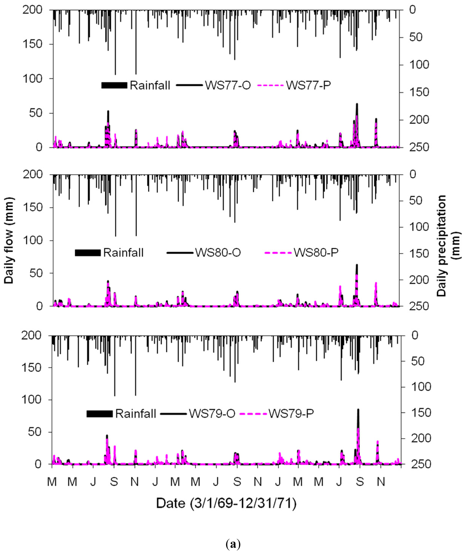
Our previous study calibrated and validated the MIKE SHE model using 5-year (2003–2007) observations of stream flow and water table from a sub-watershed (WS80) of this study watershed [45]. The model performance was evaluated using stream flow and water table observed in different time periods and different sub-watersheds for this study. In order to have the model yield the same prediction capability on all sub-watersheds in this paired system, the stream flow and water table from both the sub-catchments of control and treatment were used for the model validation. However, the validation using continuous daily observations of flow and water table in the same period for all sub-catchments was limited due to missing data in stream flow and water table. Therefore, two periods were used for testing the model performance in simulating daily stream flow. The first period, from March of 1969 to the end of 1971 (34 months), was before the Hurricane Hugo (September of 1989) and the second period, from 2005–2007 (36 months), was after the hurricane. The climatic conditions in these two periods covered dry, wet and normal hydrological years with annual precipitation ranging from 1041 mm in 2007 to 1694 mm in 1971. The average annual precipitation in these two validation periods was 1396 mm, 26 mm higher than the long-term mean of 1370 mm (1946–2007), with 1515 mm of average annual precipitation in the first validation period (1969–1971) and 1284 mm in the second period (2005–2007), respectively.
The model was also evaluated using daily water table observations from spatially distributed manual wells between 1992 and 1994 and two automatic wells between 2005–2007 on WS77 and WS80. However, the model was only validated using both daily water table and daily stream flow observations on WS77 and WS80 for second validation period (2005–2007) due to data missing.
The model performance was evaluated employing widely used quantitative method, coefficient of determination (R2) and model efficiency (E) [82]. The percent bias (PBIAS) between simulated and observed values and RMSE-observations standard deviation ratio (RSR) which is the ratio of the root mean squared error (RMSE) to SD (standard deviation) was also used to evaluate the model performance [83]. The percent bias is calculated as
The model evaluated with the above approaches was then used to simulate stream flow and water table dynamics with 58-year (1950–2007) of climate observations. The simulated daily results were integrated into monthly and yearly values to compare to the observations and assess the long-term impact of climate variability on stream flow and water table dynamics in this area.
3. Results and Discussion
3.1. Model Performance
The results of model testing using daily stream flow data are presented in Figure 2a,b and Table 2. Although these figures showed that MIKE SHE captured the stream flow dynamics under different precipitation conditions, there were some substantial under-predictions and small over-predictions. The model under predicted the flow for WS77 and slightly over predicted for WS80 and WS79 on August 11 of 1969. The under-prediction for WS77 was most likely due to the spatial difference in precipitation [84] because the precipitation for this month was missing at the onsite weather station for WS77 and the replaced precipitation was obtained from an adjacent onsite station, about 1.5 km away. However, the mean measured stream flow (45.3 mm) from the two sub-catchments (WS77 and WS80) of WS79 for August 11 of 1969 was very close to the simulated value (44.6 mm) for WS79.
The model slightly over-predicted the stream flow on July 14 and August 24 of 2005 for all sub-catchments; reversely, the model substantially under predicted the flow for all sub-watersheds on August 26 of 1971. These over and under predictions are mostly resulted from employing replaced precipitation for summer storm events because all the onsite precipitation measurements were missing and replaced precipitation was obtained from SHQ for this simulation. The observed stream flow from the three gauging stations for August 26, 1971 varied substantially, indicting differences in spatial distribution of precipitation not only between SHQ and the study site (about 3 km away), but also among the sub-watersheds of WS79, during this summer storm event (Figure 2a). These results suggest that there is a large uncertainty to simulate the stream flow in summers for these first-order watersheds using a precipitation data from other sites.
The E was 0.52–0.75 for daily flow and 0.81–0.95 for monthly flow in the two time periods (1969–1971 and 2005–2007). The R2 was 0.61–0.75 for daily flow and 0.84–0.96 for monthly flow, respectively, on WS77, WS80 and WS79 in the same periods (Table 2); and the R2 and E were 0.78 and 0.77, respectively, for monthly flow between 1965 and 2007. These qualitative (Figure 2a–c) and quantitative (E and R2) results showed that the simulation was in agreement with the measurements. Moriasi et al. [83] suggested that the RSR and PBIAS should also be used to judge model performance. From this simulation, RSR was 0.44–0.66 for daily flow and 0.05–0.35 for monthly flow, respectively; and PBIAS was between −15 and 3.6% for daily and monthly flow. Based on the suggestions of Moriasi et al. [83] that E > 0.75 for monthly flow represents a “very good” model performance and the values of RSR (≤0.7) and PBIAS (±25%) should be within the ranges of the reasonable model performance ratings, MIKE SHE was applicable for predicting stream flow on WS79.
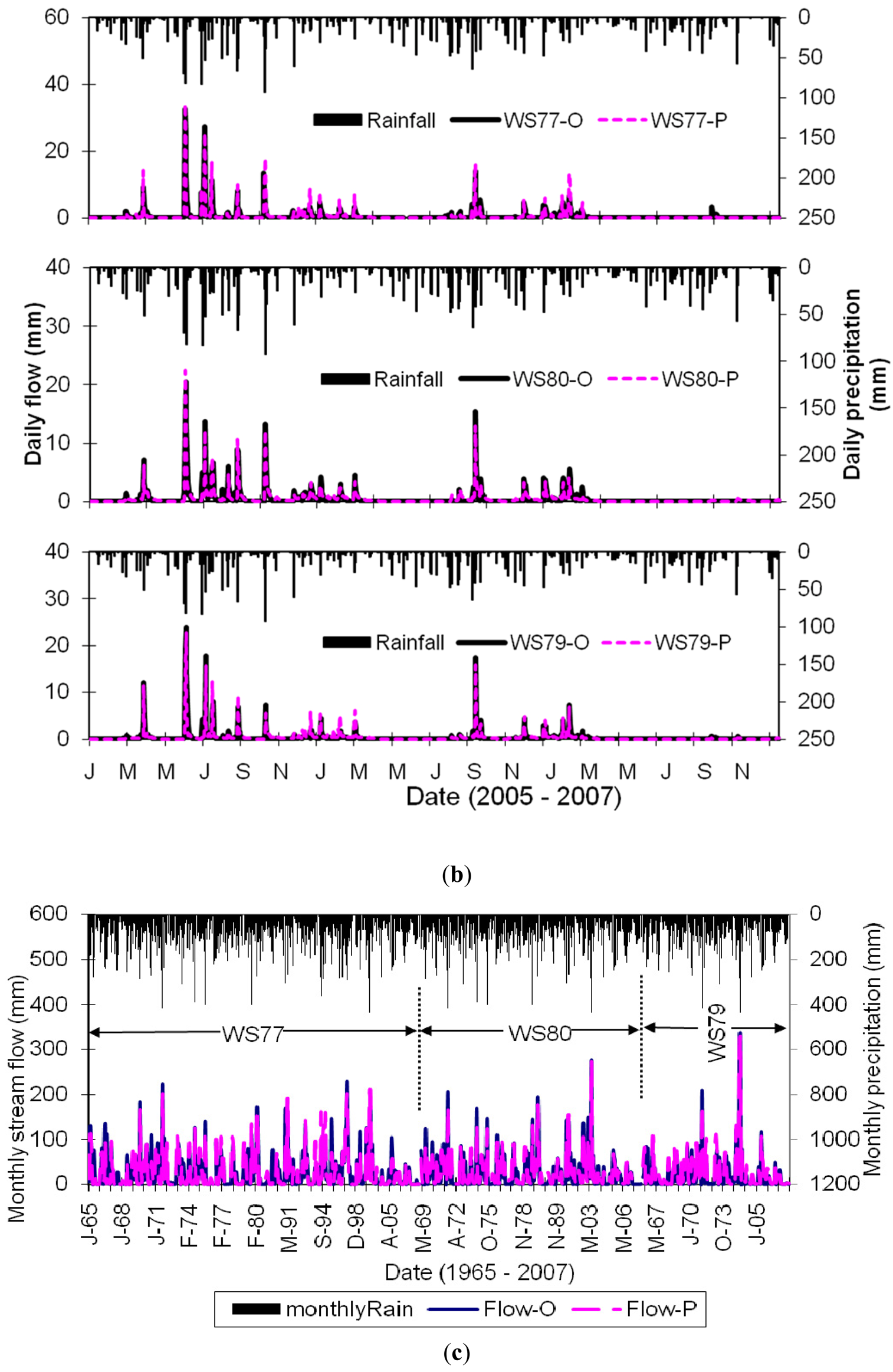
The observed and simulated daily average water table depth for WS77 and WS80 between 1992 and 1994 (Figure 3a) showed that MIKE SHE was able to capture the water table dynamics in this study site. However, it slightly under predicted the water table depth for WS80 in 1992 and the spring of 1993, and over predicted for both WS77 and WS80 during the period from the fall of 1993 to spring of 1994. The over-prediction of water table depth for both the sub-catchments seems to be a systematic error. However, the simulated stream flow for WS77 between 1993 and 1994 was in good agreement with the observation, with R2 of 0.83, E of 0.81 and the regression slope of 1.05 between simulation and observation. Because of the lack of the observed stream flow data and other hydrological components for WS79 and WS80, it is very difficult to estimate the source of the systematic error. Similarly, we couldn't evaluate whether the under-prediction of water table for WS80 was related to over-prediction of other hydrological components. The water table depth observed and simulated for two automatic wells on WS77 and WS80 was presented in Figure 3b. The plot showed that the simulated water table for both wells was in good agreement with the observations.
The E was 0.85 and 0.80 for daily water table depth on WS77 and WS80, respectively, during the period from 1992 to 1994, and 0.53 and 0.79 for the period from 2005 to 2007; the R2 was 0.87 and 0.81, and 0.69 and 0.82; the RSR was 0.42 and 0.62; the PBIAS was 3.9 and −0.08 for the same periods; and the difference in mean water table depth between the observation and simulation for the two validation periods was less than 10 cm (between −8.6 and 1.6 cm for WS77 and −3.5 and 3.9 cm for WS80). These qualitative (Figure 3a,b) and quantitative assessments show that MIKE SHE is applicable to model water table dynamics for this study site.
3.2. Climate Variability
3.2.1. Temperature
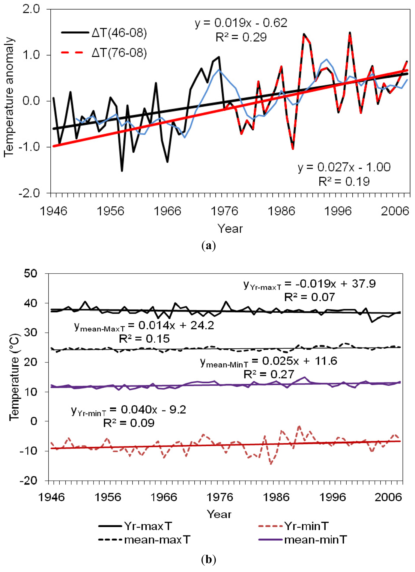
The anomaly of annual mean temperature for the 63-year period from 1946 to 2008 (Figure 4a) showed that the air temperature on SEF significantly (P < 0.01) increased at an average rate of 0.19 °C per decade. We divided the temperature variability into three sub-periods, 1946–1968, 1969–1980 and 1981–2008, based on the 5-year running averages. The warmest year in the 23-year period (1946–1968) was 1964 with a mean daily temperature (MDT) of 18.9 °C, and the coolest year was 1958 with MDT being 17 °C. The mean annual temperature was 18.0 °C in the 23-year period. Although there was a substantial temperature fluctuation in this period, the temperature did not increase but slightly decreased. However, temperature has substantially increased since 1969 in this area. The warmest year was 1975 in the second period (1969–1980), with MDT being 19.5 °C, about 0.6 °C higher than the MDT of the warmest year in the first period (1946–1968). The lowest MDT was recorded in 1979 (17.8 °C) in the second period, but it was about 0.8 °C higher than the MDT of the coolest year in the first period. The mean annual temperature in this 12-year period from 1969 to 1980 was 18.6 °C, about 0.6 C higher than first period. It was shown that temperature increased at a very high average rate in the 12-year period due to consecutive six warm years occurred from 1970 to 1975.
The year 1998 was considered to be the first warmest year experienced by human being in the period of instrumental measurements from the late 1800s to the end of last century because of the strongest El Niño in the last century, but 1990 was the first warmest year on SEF in the period from 1946–2008. The MDT in both 1990 and 1998 was 20 °C, about 1.2 and 0.5 °C higher than the MDT of the warmest years in the first and second periods, and 2 and 1.4 °C higher than the mean annual temperature in these two periods, respectively. The coolest year in the third period (1981–2008) was 1988 with MDT of 17.5 °C, 0.5 °C higher than the MDT of coolest year in the first period, but 0.3 °C lower than that in the second period. The average annual temperature in this period was 18.9 °C, about 0.9 and 0.3 °C higher than that in first and second periods, respectively. It was shown that, although two extremely high temperature years (1990 and 1998) occurred in this period, the magnitude of increase of the mean annual temperature in the 28-year period (1981–2008) was lower than that in the second period (12-year, 1969–1980), which was likely impacted by multi-decade climate fluctuation. However, the mean temperature was still increasing.
There was a significant linear increase in the annual mean daily minimum temperature at a rate of 0.26 °C per decade (P < 0.01) on SEF since 1946 (Figure 4b). This rate was higher than the rising rate of annual average of mean daily temperature (0.19 °C per decade) in the same period. Although the increase in the mean daily maximum temperature was significant (P < 0.01) in the same period, the increase magnitude (about 0.13 °C per decade) was less than the increase in mean daily minimum temperature. These results suggest that the local warming mostly influenced daily minimum temperature larger than the daily maximums. There was an upward trend in yearly minimum temperature (i.e., the lowest temperature recorded in a year) and downward trend in yearly maximum (the highest temperature observed in a year) since 1946 (P ≤ 0.05) (Figure 4b), and the fluctuation in yearly minimum temperature was large. The changes in yearly minimum and maximum indicate that the warming adds less extra degrees to extremely high and low temperature on SEF in the 63-year period.
The temperature on SEF significantly increased linearly in summers (June–August) (P < 0.01), falls (September–November) (P < 0.01) and springs (March–May) (P < 0.05), at a rate of about 0.18, 0.24 and 0.14 °C per decade, respectively. Linear temperature increase in winters (December–February) was not significant (0.1 > P > 0.05) due to large fluctuations of the yearly minimum temperature, especially due to the two consecutive warm winters in 1948 and 1949, about 2.8 °C higher than the 63-year average, and two consecutive cold winters in 1976 and 1977, about 3.0 °C lower than the long-term average. However, the average winter temperature (10.4 °C) in the period from 1970–2008 was 0.8 °C higher than the average (9.6 °C) in the period from 1946–1969, increased at a rate of about 0.2 °C per decade in the 39-year period. These results show that the warming yields not only hot summers for us, but also warmer other seasons. Although there was not a significant linear upward trend (p < 0.1) in the number of days with high temperature (>37 °C) in a year, the annual average of 2.1 days with higher than 37 °C temperature in the period from 1970–2008 were over twice as many as the average (0.83 days) in the period from 1946–1969. This result shows that the warming yields more hot days in which the mean daily air temperature is higher than human body temperature in this coastal area.
3.2.2. Precipitation
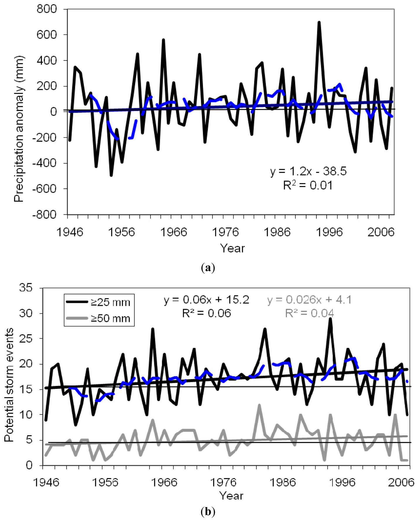
The year-to-year variability of precipitation on SEF was large in the last 63 years. It ranged from 835 mm in 1954 to 2026 mm in 1994. The average annual precipitation in the 63-year period was 1370 mm. There were three very dry years, 1951, 1954 and 1956, with the annual precipitation of about 66, 61, and 68% of the average annual value, respectively, in the 63-year period, and all three years recorded rainfall below 1000 mm. The extremely wet year was 1994 with 2026 mm precipitation, which was about 656 mm (48%) higher than the long-term average. The variations in annual precipitation exhibited an upward trend since 1946 (Figure 5a). However, the increase was insignificant (P > 0.1). This upward trend probably resulted from a lower precipitation period with three consecutively dry years in the 1950's, or from multi-decade precipitation fluctuation. The insignificant relationship between the temperature rise (Figure 4a) and annual precipitation increase (Figure 5a) (P ≫ 0.1) shows that local warming does not bring more rain, similar to the finding that global warming does not bring more rain to subtropical areas as reported by Zhang et al. [11].
The monthly mean precipitation was 114 mm in the last six decades. The maximum monthly precipitation was 437 mm in July of 1964, and the minimum was 0 mm in October of 2000. Precipitation in summers (June–August) was much higher than other seasons, yielding about 39% of annual precipitation in the last 63 years, but there were no substantial differences among the other seasons (20–21%). This is consistent with a recent study by Amatya and Skaggs [54] for a coastal forest site in North Carolina who found the 21-year mean summer rainfall as 37% of the mean annual total. The changes in seasonal precipitation were extremely small in the last six decades with only a slight upward trend in falls and winters, but there was a downward trend in springs and summers. Therefore, the warming is likely to potentially bring more spring and summer droughts to this area, which are detrimental to forests [85], especially for those summer droughts due to high evapotranspiration demands in summers.
Although there was not a significant upward trend in potential storm events (>25 mm and >50 mm precipitation events) in the last 63 years (P > 0.05) (Figure 5b), the annual average events with >25 mm precipitation and with >50 mm between 1970 and 2008 were about 13 and 21% higher than those in the period from 1946–1969, respectively. The annual average large storm events (>50 mm) were 4.4 times per year in the period from 1946–1981 and 5.7 times per year from 1982–2008, respectively. This demonstrates that climate change can bring more large size storm events to this area, besides higher temperature.
3.3. Climate Variability Impact on Stream Flow and Water Table
3.3.1. Impact on Stream Flow
In order to determine whether the Hurricane Hugo influences the runoff coefficient (ROC) (percentage of stream flow to precipitation in a unit time), and whether some differences in tree species can significantly alter the ROC, the observed ROC on WS77 before and after the hurricane was compared to the ROC in the same periods on WS80, respectively. The observed average monthly stream flow to monthly precipitation (MROC, %) on WS77 and WS80 was about 19.3% (201 months) and 19.6% (146 months), respectively, before the hurricane (1964–1981), and 21.6% (156 months) and 20.6% (92 months) after the hurricane (1990–2007). It seems that there are slight differences in the MROC between the two sub-watersheds after the hurricane, and there may be a small difference between pre-hurricane and post-hurricane for both sub-watersheds. However, the difference in the MROC between the two sub-watersheds might have also resulted from a bias in flow data availability in the observation periods as flow monitoring on WS80 did not start until late 1968. Compared to the observations from the same periods (146 months between 1968 and 1981 for pre-hurricane, and 92 months between 1990 and 2007 for post-hurricane) for both sub-watersheds, the MROC was 19.7 and 19.6% on WS77 and WS80, for pre-hurricane, and 19.5 and 20.6% for post-hurricane, respectively. The results from the same observation periods showed that there was not a substantial difference in the MROC between WS77 and WS80 before the hurricane, but there was a small difference after the hurricane, or the MROC on WS77 was smaller than WS80. This is in agreement with the smaller rate of stream flow on WS77 compared to WS80 after the hurricane than the rate before the hurricane as reported by Amatya et al. [49]. This result indicated that the difference in the MROC between these two sub-watersheds after the hurricane might be potentially resulted from the differences in vegetation, more pine trees on WS77 than WS80, with different water use efficiency [54]. These authors outlined methods to test possible hypotheses including the effect of post-hurricane recovery on vegetation and ET for the reversal observed in flows between these two subwatersheds before the hurricane (1968–81) and ten years after the hurricane (1993–2003).
However, the difference in the MROC between the pre- and post-hurricane on WS80 (19.6 vs. 20.6) might reflect the impact of Hurricane Hugo on stream flow on WS79 (see more discussion on the impact of the hurricane below). This result is similar to those, with the ratio of annual ROC between 1990 and 1993 (after the hurricane) being higher than the ROC between 1977 and 1981 (before the hurricane) on WS80, as reported by Wilson et al. [40].
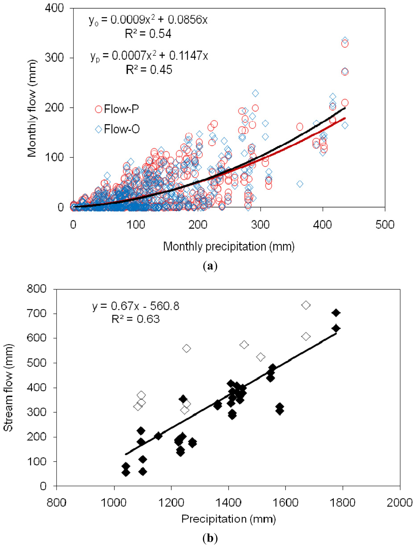
Both the observed and simulated results showed a significantly non-linear (quadratic polynomial) relationship between the monthly flow and monthly precipitation (p ≪ 0.01; Figure 6a). The average annual stream flow was 22.8% of the mean annual precipitation from observation in the period from 1965–2007 and 23.4% from the simulation in the same period; the observed annual stream flow proportionally varied at a rate of 2.5% with one percentage of precipitation change (Figure 6b), approximate to the simulated value (2.4%) using eight climate change scenarios [52]. This value indicates that precipitation obviously influences the stream flow on this second-order watershed, and it is comparable to the stream flow response to changes in precipitation in the Trend River basin in North Carolina where a 23% increase in stream flow corresponded to a 10% increase in precipitation [86]. These results are, however, very different from the small drained forest land in eastern NC where the 10% increase in annual rainfall increased the stream flow by as much as 78%, on average [54].
Figure 6b exhibited the impact of Hurricane Hugo, categorized as IV storm, on the stream flow of WS77 and WS80 on the SEF. The blank and black diamonds in the figure represent the overall observed relationship between annual stream flow and precipitation during the period from 1965–2007, but the blank ones represent the relationship for only the 14 years (1990–2003) after the hurricane in 1989 (only 10 observations available due to missing data), showing that the observed annual stream flow in the period from 1990–2003 is above the mean trend line. However, the average annual precipitation in those years was about 43 mm lower than the average in the observation period (1965–2007), and 70 mm lower than the long-term average (1370 mm). For example, precipitation was 1095 mm in 1990, 275 mm less than the long-term average, but the observed and simulated annual stream flow was 33.7 and 33.3% of annual precipitation, respectively, for this year, about 10 percentages higher than the average from 1965–2007 (22.8% from observation and 23.7% from simulation for same time periods). Although both observation and simulation showed the impact of the hurricane on the stream runoff coefficients (ROC), the simulated impact period was slightly shorter than the observed; the observed impact on stream flow could be between 1990 and 2003 (with data missing between 1999–2002), but the simulated impact was in the period from 1990–2001. However, this impact period was longer than the duration (1990–1993) reported by Amatya et al. [49], and Wilson et al. [40]. The high ROCs observed in those years after the hurricane was attributed to the hurricane damage of over 80% of the forest canopies at this site [64], resulting in a decrease in evapotranspiration (ET). However, the flow recovered as the vegetation regenerated (about 10 years) after the hurricane [54]. Some of our results here are also consistent with a study conducted by Shelby et al. [39] for effects of extreme weather conditions on stream flow in North Carolina watersheds.
The simulated stream flow dynamics in last 58 years (1950–2007) showed that the stream flow of WS79 followed the precipitation pattern in this site with an R2 of 0.86 (p < 0.01, n = 58), thus, high annual precipitation yields large yearly flow on the watershed, which is in agreement with the observation in this catchment. This pattern is similar to the results from forested watersheds in Florida and North Carolina as reported by Lu et al. [51] and Amatya et al. [54]. The simulated average annual stream flow (1950–2007) on WS77 (319 mm/yr) is overall approximate to the flow on WS80 (320 mm/yr). However, the average annual stream flow on WS79 (361 mm/yr) is higher than those on its two sub-watersheds, WS77 and WS80. This can be attributed mostly to the difference in base flows due to a higher base flow from the second-order watershed than its sub-watersheds [13] and some possibly to the increased open areas like service roads in the larger watershed. Similar to observations, the simulated results showed that the annual ROC on WS77 for the period from 1965–1989 (before the hurricane) was overall approximate to WS80 based on the regression model between the simulated results for WS77 and WS80 with a slope of 1.000, intercept of zero and R2 of 0.95 (n = 25), but the ROC on WS77 after the hurricane (1990–2007) was slightly smaller than WS80 with a slope of 0.98 and R2 of 0.99 (n = 18), which reflects the model captured the impact of the differences in vegetation on hydrology on these two sub-watersheds after the hurricane.
The observed monthly runoff coefficient in the period from 1965–2007 showed a downward trend with an increase in temperature that occurred in March, May–September, November and December, but not in January, February, April and October. However, both the observation and simulation results did not find a significant correlation between the changes in temperature and stream flow on this watershed in the period from 1965–2007 although the stream flow can reduce at a rate of about 5% with an increase in temperature of 1 °C [52,86]. This might be due to the fact that the temperature rise is small (about 0.19 °C per decade) and the precipitation change is large (from 800–2000 mm) in this area. The seasonal results showed an insignificant downward trend in stream flow with an increase in temperature in springs and falls (P ≥ 0.05) that was larger than in summers (P > 0.2), and an insignificant upward trend (P ≫ 0.1) was observed in winters in this area. However, the simulated downward trend of the MROC in summers changed slightly after 1969 (P altered from >0.2 to ≥ 0.05), which was likely due to an insignificant temperature rise before 1969 and a substantial increase in temperature since 1970. These results indicate that temperature change can influence the stream flow in this second watershed, but its impact on stream flow is smaller than that of the precipitation due to highly variable precipitation in this area.
3.3.2. Impact on Water Table
The results from the observations and simulations showed that precipitation influenced the water table depth (WT) at this site (Figure 3a,b). The simulated annual mean WT was a function of logarithmic yearly precipitation (i.e., [WT, cm] = a × ln[precipitation, mm] + b, where a and b are coefficients) (P < 0.02), the higher the annual precipitation, the higher the mean WT this watershed has. Water table level is, therefore, near the surface during wet periods (Figure 3a,b), over 2.0 m below the surface during dry periods. These results are similar to those obtained by Amatya et al. [44] for the adjacent Turkey Creek watershed as well as for the drained pine forest in eastern NC Amatya et al. [54] where the authors found a linear relationship with their 17-year (1988–2004) data. Harder et al. [66] found a significant relationship between WT and stream flow on WS80 (P < 0.02). Their result implied that the WT on this watershed was substantially affected by precipitation due to a strong significant relationship between precipitation and stream flow on the same watershed (P ≪ 0.01). Amatya et al. [54] also reported a significant linear relationship between the annual stream flow and logarithmic of water table depth.
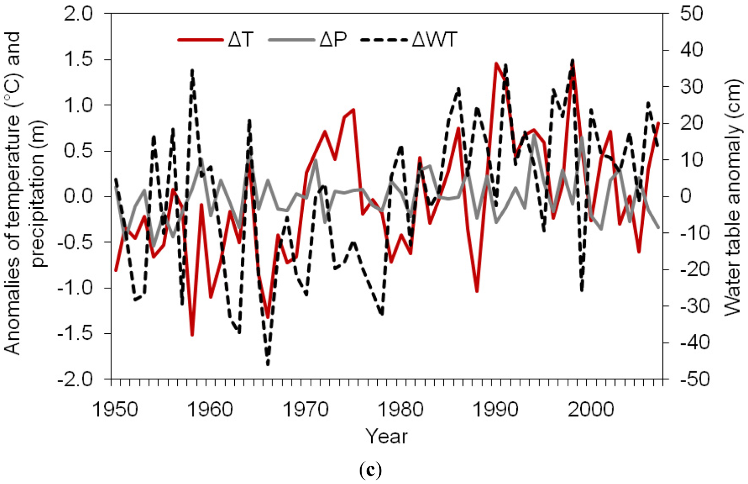
The temporal fluctuation of water table level was large on the first-order watersheds on SEF (Figure 3a,b, Figure 6c). The water table level was high in most of winter-spring (December–April) periods. However, precipitation in winters and springs (about 20% of annual precipitation on average) is lower than that in summers (≈39%). The high water table level in winters and/or springs mainly resulted from a low demand in evapotranspiration (ET). High water table level in other seasons is related to high precipitation. The WT in dry periods, especially in dry summers, was over 2 m below the ground surface on these first-order watersheds, and the difference in WT between upland and riparian zone in dry periods was over 1 m. Nevertheless, a large area of the watershed WS79 is saturated during rain and wet periods [52]. Although average precipitation in summers was about 1.8 times as much as that in springs and winters, the average water table in summers was generally lower than springs and winters, showing that ET is one of the key factors influencing the water table on these first and second order watersheds.
Figure 6c shows that the temporal changes in WT on WS79 were complex due to the synergy of temperature, for that matter PET, and precipitation. For example, the highest WT level occurred in 1998, but this year was one of the warmest years (20 °C of mean daily temperature) since 1946. However, high WT in 1998 was most likely related to an abnormal annual precipitation pattern because over 78% of annual precipitation occurred in the winter (December, January and February) and the spring (March–May) when the ET demand was low. This result shows that the WT on WS79 can be substantially influenced by the changes in seasonal precipitation.
The water table level in 1958 with 1460 mm precipitation was the second highest in the 58-year (1950–2007) period, but the water level in 1959 with 1780 mm precipitation was about 29 cm lower than that in 1958. This is a perfect example of a completely reversed pattern of the expected normal relationship between WT and precipitation in this area, i.e., the water table level rises with an increase in precipitation. This phenomenon likely resulted from two factors, seasonal storms and temperature. 1958 was the coolest year in the 58-year period from 1946–2008 (Figure 4a), with only 17 °C as average daily temperature. The average daily temperature in 1959 was 1.5 °C higher than 1958, most likely resulting in a higher evapotranspiration demand with a subsequent lowering of water table than in 1958. The other potential factor might be the magnitude of storms in the summers because there were no differences in precipitation in the winter, spring and fall between these two years. There were six storm events with over 70 mm precipitation and two events with over 100 mm in 1959; but there were only two storm events with over 55 mm precipitation in 1958. Higher precipitation in 1959 mainly contributed by the larger summer storms than in 1958 might not have resulted in a substantial higher water table for these headwater areas in that year. It was concluded, therefore, that storms with high precipitation in the summer contribute to only a small rise in the water table on these first-order watersheds although the water table generally rises with an increase in precipitation in this area.
The comparison of the WT in 1988 and 1990 indicates that temperature substantially influences the WT dynamics on these first-order watersheds. The WT in 1988 was substantially higher than that in 1990. However, there was neither substantial difference in annual and seasonal precipitation between these two years, nor was there a difference in magnitude of storms. The main difference between these two years was temperature and biomass, with temperature in 1988 being 2.5 °C lower than 1990 and biomass in 1990 being lower than in 1988, due to the destruction of the forest canopy by Hurricane Hugo in 1989 [64]. Generally, the water table and the annual ROC in 1990 should be higher than those in 1988 due to low demand in transpiration if precipitation condition was similar between these two years, but the result was reversed for water table, and in agreement for the stream flow. This result showed that the WT on SEF was influenced by the synergy of temperature and the vegetation biomass impacted by the hurricane. Similarly, the difference in WT between 1969 and 1970 also indicated the impact of temperature on WT. There were not substantial differences in biomass and precipitation between the two years. However, temperature in 1969 was 1 °C lower than 1970. The WT from observation and simulation in 1969 was substantially (over 20 cm) higher than that in 1970. These results indicate that temperature, for that matter ET, is one of important factors which influence the WT on these first-order watersheds, and that local warming without bringing more rain can reduce the water table level on this study catchment.
4. Conclusions
The observations and simulations show that there may be substantial hydrologic alterations induced by climate change in forested watersheds on the lower coastal plain. The long-term climate observations indicate that there hasn't been a substantial increase in annual precipitation in this area, but that air temperature has increased. Due to the large variability in precipitation, we could not detect change in stream flow over the period. The coastal plain watersheds are subject to tropical storms that can alter the hydrology by affecting forest composition and structure.
Continued increase in regional temperature will likely cause a decrease in stream flow and water table level on these first- and second-order watersheds, because an increase in temperature can lead to an increase in evapotranspiration. Based on the projections of the hydrologic changes of this forested watershed, using the synthesis of the observations and simulations, the extent of areas with wetland hydrology, dependent on shallow water table in this study catchment, will either shrink or disappear in the future; this is because the climate change may substantially raise the air temperature but may not bring an adequate precipitation increase to this watershed containing both wetlands and uplands to compensate for the increase in ET demands caused by temperature increase. The results from both the observation and simulation for the impacts of Hurricane Hugo in 1989 indicate that the forest hydrology of this catchment is obviously impacted by the change in vegetation coverage.


| Parameter | Value |
|---|---|
| Plant rooting depth [mm] | 300–700 |
| Leaf area index (LAI) [m2/m2] | 0.2–6.6 (2.8 on average) |
| Potential evapotranspiration (PET) [mm/d] | 0.0–7.5 |
| Surface detention storage [mm] | 10–240 |
| Manning M (ground surface/stream bed) [m1/3/s] † | 30/60 |
| Initial water depth [m] | 0 |
| Soil water content at saturated conditions [m3/m3] | 0.4–0.496 |
| Soil water content at field capacity [m3/m3] | 0.3–0.458 |
| Soil water content at wilting point [m3/m3] | 0.2–0.38 |
| Infiltration [10−6 m/s] | 1–800 |
| ET surface depth [m] | 0.2 |
| Horizontal hydraulic conductivity [10−6 m/s] | 10–100 |
| Vertical hydraulic conductivity [10−6 m/s] | 1–80 |
| Drainage depth [m] | 0.05–1.20 |
| Drainage time constant [/s] | 1 × 10⁻⁷ |
| Coefficient of canopy interception [mm] | 0.22 |
*Daily PET is based on Penman-Monteith (P-M) [73].†Manning M = (Manning's n)−1; M = 30 is used for ground surface, M = 60 for stream bed
| watershed | 1969-1971 | 2005-2007 | |||||||||||
|---|---|---|---|---|---|---|---|---|---|---|---|---|---|
| O | P | R2 | E | RSR | PB | O | P | R2 | E | RSR | PB | ||
| WS77 | daily | 1.35 | 1.35 | 0.82 | 0.80 | 0.44 | 0.69 | 0.51 | 0.52 | 0.61 | 0.52 | 0.63 | −1.0 |
| monthly | 41.2 | 41.0 | 0.94 | 0.94 | 0.20 | 0.69 | 15.4 | 15.6 | 0.91 | 0.91 | 0.31 | −1.0 | |
| WS80 | daily | 1.26 | 1.34 | 0.69 | 0.66 | 0.58 | −6.5 | 0.46 | 0.52 | 0.75 | 0.75 | 0.50 | −12 |
| monthly | 38.4 | 40.9 | 0.93 | 0.92 | 0.30 | −6.5 | 14.0 | 15.7 | 0.96 | 0.94 | 0.24 | −12 | |
| WS79 | daily | 1.18 | 1.37 | 0.78 | 0.77 | 0.48 | −16 | 0.53 | 0.63 | 0.68 | 0.64 | 0.44 | −14 |
| monthly | 36.0 | 41.8 | 0.90 | 0.88 | 0.37 | −16 | 16.2 | 19.1 | 0.96 | 0.95 | 0.35 | −14 | |
*O is mean observation; P is mean prediction; R2 is coefficient of determination; E is model efficiency; RSR is the ratio of Root mean squared error (RMSE) to standard deviation (SD); PB is percent bias between observation and simulation (PBIAS).
References
- Arnell, N.W. The effect of climate change on hydrological regimes in Europe: A continental perspective. Glob. Environ. Change 1999, 9, 5–23. [Google Scholar]
- Nijssen, B.; O'Donnell, G.M.; Hamlet, A.F.; Lettenmaier, D.P. Hydrologic sensitivity of global rivers to climate change. Clim. Change 2001, 50, 143–175. [Google Scholar]
- Barnett, T.P.; Adam, J.C.; Lettenmaier, D.P. Potential impacts of a warming climate on water availability in snow-dominated regions. Nature 2005, 438, 303–309. [Google Scholar]
- Huang, Y.; Zou, Y.; Huang, G.; Maqsood, I. Flood vulnerability to climate change through hydrological modeling. Water Int. 2005, 30, 31–39. [Google Scholar]
- Kundzewicz, Z.W.; Mata, L.J.; Arnell, N.W.; Doll, P.; Jimenez, B.; Miller, K.; Oki, T.; Sen, Z.; Shiklomanov, I. The implicastions of projected climate change for freshwater resources and their management. Hydrol. Sci. 2008, 53, 3–10. [Google Scholar]
- Sun, G.; McNulty, S.G.; Moore Myers, J.A.; Cohen, E.C. Impacts of multiple stresses on water demand and supply across the Southeastern United States. JAWRA 2008, 44, 1441–1457. [Google Scholar]
- Chung, E.S.; Lee, K.S. Identification of spatial ranking of hydrological vulnerability using multi-criteria decision making techniques: Case study of Korea. Water Resour. Manag. 2009, 23, 2395–2416. [Google Scholar]
- IPCC. Climate Change 2007: The Physical Science Basis. In Contribution of Working Group I to the Fourth Assessment Report of the Intergovernmental Panel on Climate Change; IPCC: Paris, France; February; 2007. [Google Scholar]
- Wentz, F.J.; Ricciardulli, L.; Hilburn, K.; Mears, C. How much more rain will global warming bring? Science 2007, 317, 233–235. [Google Scholar]
- Lambert, F.H.; Stine, A.R.; Krakauer, N.Y.; Chiang, J.C.H. How Much Will Precipitation Increase With Global Warming? EOS Trans. AGU 2008, 89, 193. [Google Scholar]
- Zhang, X.; Zwiers, F.W.; Hegerl, G.C.; Hugo Lambert, F.; Gillett, N.P.; Solomon, S.; Stott, P.A.; Nozawa, T. Detection of human influence on twentieth-century precipitation trends. Nature 2007, 448, 461–465. [Google Scholar]
- Amatya, D.M.; Sun, G.; Skaggs, R.W.; Chescheir, G.M.; Nettles, J.E. Hydrologic Effects of Global Climate Change on a Large Drained Pine Forest. Hydrology and Management of Forested Wetlands: Proceedings of the International Conference; Williams, T.M., Nettles, J.E., Eds.; ASABE: Joseph, MI, USA, 8 April 2006. [Google Scholar]
- Amatya, D.M.; Radecki-Pawlik, A. Flow Dynamics of Three Experimental Forested Watersheds in Coastal South Carolina, U.S.A. Acta Sci. Pol. Form. Cirtumiectus 2007, 6, 3–17. [Google Scholar]
- Middelkoop, H.; Daamen, K.; Gellens, D.; Grabs, W.; Kwadijk, J.C.J.; Lang, H.; Parmet, B.W.A.H.; Schadler, B.; Schulla, J.; Wilke, K. Impact of climate change on hydrological regimes and water resources management in the Rhine basin. Clim. Change 2001, 49, 105–128. [Google Scholar]
- Gosain, A.K.; Rao, A.; Basuray, D. Climate change impact assessment on hydrology of Indian river basins. Curr. Sci. 2006, 90, 346–353. [Google Scholar]
- Steele-Dunne, S.; Lynch, P.; McGrath, R.; Semmler, T.; Wang, S.; Hanafin, J.; Nolan, P. The impacts of climate change on hydrology in Ireland. J. Hydrol. 2008, 356, 28–45. [Google Scholar]
- Hartig, E.K.; Grozev, O.; Rosenzweig, C. Climate change, agriculture and wetlands in Eastern Europe: Vulnerability, adaptation and policy. Clim. Change 1997, 36, 107–121. [Google Scholar]
- Johnson, W.C.; Millett, B.V.; Gilmanov, T.; Voldseth, R.A.; Guntenspergen, G.R.; Naugle, D.E. Vulnerability of north prairie wetlands to climate change. BioScience 2005, 55, 863–872. [Google Scholar]
- Acreman, M.C.; Blake, J.R.; Booker, D.J.; Harding, R.J.; Reynard, N.; Mountford, J.O.; Stratford, C.J. A simple framework for evaluating regional wetland ecohydrological response to climate change with case studies from Great Britain. Ecohydrology 2009, 2, 1–17. [Google Scholar]
- Titus, J.G.; Hudgens, D.E.; Trescott, D.L.; Craghan, M.; Nuckols, W.H.; McCue, C.H.; O'Connell, J.F.; Tanski, J.; Wang, J. State and local governments plan for development of most land vulnerable to rising sea level along the US Atlantic coast. Environ. Res. Lett. 2009, 4. [Google Scholar] [CrossRef]
- Burkett, V.; Kusler, J. Climate change: Potential impacts and interactions in wetlands of the United States. JAWRA 2000, 36, 313–320. [Google Scholar]
- Winter, T.C. The vulnerability of wetlands to climate change: A hydrologic landscape perspective. JAWRA 2000, 36, 305–311. [Google Scholar]
- Scavia, D.; Field, J.C.; Boesch, D.F.; Buddemeier, R.W.; Burkett, V.; Cayan, D.R.; Fogarty, M.; Harwell, M.A.; Howarth, R.W.; Mason, C.; et al. Climate change impacts on U.S. coastal and marine ecosystems. Estuaries 2002, 25, 149–164. [Google Scholar]
- Najjar, R.G.; Walker, H.A.; Anderson, P.J.; Barron, E.J.; Bord, R.J.; Gibson, J.R.; Kennedy, V.S.; Knight, C.G.; Megonigal, J.P.; O'Connor, R.E.; et al. The potential impacts of climate change on the mid-Atlantic coastal region. Clim. Res. 2000, 14, 219–233. [Google Scholar]
- Day, J.W.; Christian, R.R.; Boesch, D.M.; Yáñez-Arancibia, A.; Morris, J.; Twilley, R.R.; Naylor, L.; Schaffner, L.; Stevenson, C. Consequences of climate change on the ecogeomorphology of coastal wetlands. Estuaries Coasts 2008, 31, 477–491. [Google Scholar]
- Brooks, R.T. Potential impacts of global climate change on the hydrology and ecology of ephemeral freshwater systems of the forests of the northeastern United States. Clim. Change 2009, 95, 469–483. [Google Scholar]
- Erwin, K.L. Wetlands and global climate change: The role of wetland restoration in a changing world. Wetlands Ecol. Manag. 2009, 17, 71–84. [Google Scholar]
- Xie, Z.; Xu, X.; Yan, L. Analyzing qualitative and quantitative changes in coastal wetland associated to the effects of natural and anthropogenic factors in a part of Tianjin, China. Estuarine Coast Shelf Sci. 2010, 86, 379–386. [Google Scholar]
- Pielke, R.A.; Landsea, C.; Mayfield, M.; Laver, J.; Pasch, R. Hurricanes and global warming. BAMS 2005, 1571–1575. [Google Scholar]
- Pezza, A.B.; Simmonds, I. The first South Atlantic hurricane: Unprecedented blocking, low shear and climate change. Geophys. Res. Lett. 2005, 32. [Google Scholar] [CrossRef]
- Trenberth, K. Uncertainty in hurricanes and global warming. Science 2005, 308, 1753–1754. [Google Scholar]
- Elsner, J.B. Evidence in support of the climate change-Atlantic hurricane hypothesis. Geophys. Res. Lett. 2006, 33. [Google Scholar] [CrossRef]
- Landsea, C.W.; Harper, B.A.; Hoarau, K.; Knaff, J.A. Can we detect trends in extreme tropical cyclones? Science 2006, 313, 452–454. [Google Scholar]
- Suhayda, J.N. Modeling impacts of Louisiana Barrier Islands on wetland hydrology. J. Coastal Res. 1997, 13, 686–693. [Google Scholar]
- Paerl, H.W.; Bales, J.D.; Ausley, L.W.; Buzzelli, C.P.; Crowder, L.B.; Eby, L.A.; Fear, J.M.; Go, M.; Peierls, B.L.; Richardson, T.L.; et al. Ecosystem impacts of three sequential hurricanes (Dennis, Floyd, and Irene) on the United States' largest lagoonal estuary. Proc. Natl. Acad. Sci. USA 2001, 98, 5655–5660. [Google Scholar]
- Steward, J.S.; Virnstein, R.W.; Lasi, M.A.; Morris, L.J.; Miller, J.D.; Hall, L.M.; Tweedale, W.A. The impacts of the 2004 hurricanes on hydrology, water quality, and seagrass in the Central Indian River Lagoon, Florida. Estuaries Coasts 2006, 29, 954–965. [Google Scholar]
- Abtew, W.; Iricanin, N. Hurricane effects on South Florida water management system: A case study of Hurricane Wilma of October 2005. J. Spat. Hydrol. 2008, 8, 1–21. [Google Scholar]
- Krauss, K.W.; Doyle, T.W.; Doyle, T.J.; Swarzenski, C.M.; From, A.S.; Day, R.H.; Conner, W.H. Water level observations in mangrove swamps during two hurricanes in Florida. Wetlands 2009, 29, 142–149. [Google Scholar]
- Shelby, J.D.; Chescheir, G.M.; Skaggs, R.W.; Amatya, D.M. Hydrology and water quality response of forested and agricultural lands during the 1999 extreme weather conditions in Eastern North Carolina. Trans. ASAE 2006, 48, 2179–2188. [Google Scholar]
- Wilson, L.; Amatya, D.M.; Callahan, T.J.; Trettin, C.C. Hurricane Impact on Stream Flow and Nutrient Exports for a First-Order Forested Watershed of the Lower Coastal Plain, South Carolina. Proceedings of the Second Interagency Conference on Research in the Watersheds; Coweeta Hydrologic Laboratory: Otto, NC, USA, May 2006; pp. 16–18. [Google Scholar]
- Amatya, D.M.; Skaggs, R.W.; Gregory, J. Effects of controlled drainage on the hydrology of drained pine plantations in the North Carolina coastal plain. J. Hydrol. 1996, 181, 211–232. [Google Scholar]
- Sun, G.; Callahan, T.J.; Pyzoha, J.E.; Trettin, C.C. Modeling the climatic and geomorphologic controls on the hydrology of a Carolina bay wetland in South Carolina, USA. Wetlands 2006, 26, 567–580. [Google Scholar]
- LaTorres Torres, I.B.; Amatya, D.M.; Sun, G.; Callahan, T.J. Seasonal rainfall-runoff relationships in a lowland forested watershed in the southeastern USA. Hydrol. Proc. 2010, 24. in press. [Google Scholar]
- Amatya, D.M.; Callahan, T.J.; Trettin, C.C.; Radecki-Pawlik, A. Hydrologic and Water Quality Monitoring on Turkey Creek Watershed, Francis Marion National Forest, SC. Proceedings of the 2008 South Carolina Water Resources Conference, Charleston Area Event Center, Charleston, VA, USA, Octuber 2005; pp. 14–15.
- Dai, Z.; Li, C.; Trettin, C.C.; Sun, G.; Amatya, D.M.; Li, H. Bi-criteria evaluation of MIKE SHE model for a forested watershed on South Carolina Coastal Plain. Hydrol. Earth Syst. Sci. 2010, 14, 1033–1046. [Google Scholar]
- Young, C.E.; Klawitter, R.A. Hydrology of wetland forest watersheds. Proceedings of Hydrology in Water Resources Management, WRRI Report 4; Clemson University: Clemson, SC, USA, 1968; pp. 29–38. [Google Scholar]
- Sheridan, J.M. Peak Flow Estimates for Coastal Plain Watersheds. Trans. ASAE 2002, 45, 1319–1326. [Google Scholar]
- Miwa, M.; Gartner, D.L.; Bunton, C.S.; Humphreys, R.; Trettin, C.C. Characterization of Headwater Stream Hydrology in the Southeastern Lower Coastal Plain; Final Report IAG#: DW12945840-01-0; Charleston, SC; USDA Forest Service Southern Research Station, 2003; p. 33. [Google Scholar]
- Amatya, D.M.; Miwa, M.; Harrison, C.A.; Trettin, C.C.; Sun, G. Hydrology and Water Quality of Two Order Forested Watersheds in Coastal South Carolina. Proceedings of the 2006 International Conference on Hydrology and Management of Forested Wetlands Conference, New Bern, NC, USA, 8–12 April, 2006; pp. 15–25.
- Frey, A.E.; Olivera, F.; Irish, J.L.; Dunkin, L.M.; Kaihatu, J.M.; Ferreira, C.M.; Edge, B.L. Potential impact of climate change on hurricane flooding inundation, population affected and property damages in Corpus Christi. JAWRA 2010, 46, 1049–1059. [Google Scholar]
- Lu, J.; Sun, G.; McNulty, S.G.; Comerford, N. Sensitivity of pine flatwoods hydrology to climate change and forest management in Florida, USA. Wetlands 2009, 29, 826–836. [Google Scholar]
- Dai, Z.; Trettin, C.C.; Li, C.; Amatya, D.M.; Sun, G.; Li, H. Sensitivity of streamflow and water table depth to potential climatic variability in a coastal forested watershed. JAWRA 2010, 46, 1036–1048. [Google Scholar]
- Amatya, D.; Chescheir, G.; Skaggs, R.; Fernandez, G. Hydrology of poorly drained coastal watersheds in eastern North Carolina. Presented at the 2002 ASAE Annual International Meeting/CIGR XVth World Congress, Sponsored by ASAE and CIGR, Hyatt Regency Chicago, Chicago, IL, USA, July 2002; pp. 28–31.
- Amatya, D.M.; Skaggs, R.W. Long-term Hydrology and Water Quality of a Drained Pine Plantation in North Carolina, U.S.A. Trans. ASABE submitted. 2011. [Google Scholar]
- Amatya, D.M.; Trettin, C.C. Annual Evapotranspiration of a Forested Wetland Watershed. Proceedings of the 2007 ASABE Annual International Meeting, Minneapolis, MN, USA, June 2007; pp. 17–20.
- DHI. MIKE SHE Technical Reference. Version 2005. DHI Water and Environment; Danish Hydraulic Institute: Denmark, 2005. [Google Scholar]
- Graham, D.N.; Butts, M.B. Chapter 10 flexible integrated watershed modeling with MIKE SHE. In Watershed Models; Singh, V.P., Frevert, D.K., Eds.; CRC Press: BocaRaton, FL, USA, 2005. [Google Scholar]
- Sahoo, G.B.; Ray, C.; Carlo, E.H. Calibration and validation of a physically distributed hydrological model, MIKE SHE, to predict streamflow at high frequency in a flashy mountainous Hawaii stream. J. Hydrol 2006, 327, 94–109. [Google Scholar]
- Dai, Z.; Amatya, D.M.; Sun, G.; Trettin, C.C.; Li, C.; Li, H. Evaluation of MIKE SHE and DRAINMOD for modeling effect of land use change on stream outflow in Coastal South Carolina. Proceedings of the 2008 South Carolina Water Resources Conference, Charleston, SC, USA, October 2008; pp. 14–15.
- Amatya, D.M.; Trettin, C.C. Development of watershed hydrologic research at Santee Experimental Forest, Coastal South Carolina. Proceedings of the Advancing the Fundamental Sciences: Forest Service National Earth Sciences Conference; Furniss, M.J., Clifton, C.F., Ronnenberg, K.L., Eds.; San Diego, CA, USA, October 2004; pp. 18–22. [Google Scholar]
- Hawley, N.R. The old rice plantation in and around the Santee Experimental Forest. Agric.History 1949, 23, 86–91. [Google Scholar]
- Hook, D.D.; Buford, M.A.; Williams, T.M. Impact of Hurricane Hugo on the South Carolina coastal plain forest. In Hurrican Hugo: South Carolina Forest Land Research and Management Related to the Storm; Haymond, J.L., Hook, D.D., Harms, W.R., Eds.; General Technical Report SRS-5; South Research Station, USDA Forest Service: Ashville, SC, USA, 1996; p. 540. [Google Scholar]
- Trettin, C.C.; Amatya, D.M.; Kaufman, C.; Levine, N.; Morgan, R.T. Recognizing change in hydrologic functions and pathways due to historical agricultural use—Implications to hydrologic assessments and modeling. Proceedings of the Third Interagency Conference Research in the Watersheds, Estes Park, CO, USA, 8–11 September 2008.
- Hook, D.D.; Buford, M.A.; Williams, T.M. Impact of Hurricane Hugo on the South Carolina Coastal Plain Forest. J. Coastal Res. 1991, (Special Issue 8), 291–300. [Google Scholar]
- Nix, L.E.; Hook, D.D.; Williams, J.G.; Blaircom, D.V. Assessment of Hurricane damage to the Santee Experimental Forest and the Francis Marion National Forest with a Geographic Information System. In Hurricane Hugo: South Carolina Forest Land Research and Management Related to the Storm; Haymond, J.L., Hook, D.D., Harms, W.R., Eds.; General Technical Report SRS-5; Asheville, NC, USA, 1996. [Google Scholar]
- Harder, S.V.; Amayta, D.M.; Callahan, T.J.; Trettin, C.C.; Hakkila, J. Hydrology and water budget for a forested Atlantic coastal plain watershed, South Carolina. JAWRA 2007, 43, 563–575. [Google Scholar]
- Federal Register. Changes in hydric soils of the United Sates 1994.
- Federal Register. Hydric soils of the United States 2002.
- Long, B.M. Soil Survey of Berkeley County, South Carolina; United States Department of Agriculture: Harrisburg: PA, USA, 1980. [Google Scholar]
- Abbott, M.B.; Bathurst, J.C.; Cunge, J.A.; O'Connell, P.E.; Rasmussen, J. An introduction to the European hydrological system—Systeme hydrologique Europeen, “SHE”, 1: History and philosophy of a physically-based, distributed modelling system. J. Hydrol. 1986, 87, 45–59. [Google Scholar]
- Abbott, M.B.; Bathurst, J.C.; Cunge, J.A.; O'Connell, P.E.; Rasmussen, J. An introduction to the European hydrological system—Systeme hydrologique Europeen, “SHE”, 2: Structure of a physically-based, distributed modelling system. J. Hydrol. 1986, 87, 61–77. [Google Scholar]
- Monteith, J.L. Evaporation and Environment. Proceedings of the 19th Symposium of the Society for Experimental Biology; Fogg, G.E., Ed.; Cambridge University Press: New York, NY, USA, 1965; pp. 205–234. [Google Scholar]
- Xu, C.; Singh, V.P. Evaluation of three complementary relationship evapotranspiration models by water balance approach to estimate actual regional evapotranspiration in different climatic regions. J. Hydrol. 2005, 308, 105–121. [Google Scholar]
- Hargreaves, G.H.; Samani, Z.A. Reference crop evapotranspiration from temperature. Appl. Eng. Agric. 1985, 1, 96–99. [Google Scholar]
- Amatya, D.M.; Skaggs, R.W.; Gregory, J.D. Comparison of methods for estimating REF-ET. J. Irrig. Drain. Eng. 1995, 121, 427–435. [Google Scholar]
- Gavilan, P.; Lorite, I.J.; Tornero, S.; Berengena, J. Regional calibration of Hargreaves equation for estimating reference ET in a semiarid environment. Agric. Water Manag. 2006, 81, 257–281. [Google Scholar]
- Sepaskhah, A.R.; Razzaghi, F. Evaluation of the adjusted Thornthwaite and Hargreaves-Samani methods for estimation of daily evapotranspiration in a semi-arid region of Iran. A. Agron. Soil Sci. 2009, 55, 51–66. [Google Scholar]
- Allen, R.G.; Pereira, L.S.; Raes, D.; Smith, M. Crop Evapotranspiration: Guidelines for Computing Crop Water Requirements-FAO Irrigation and Drainage Paper, Volume 56; Food and Agriculture Organization: Rome, Italy, 1998. [Google Scholar]
- Lloyd, F.T.; Olson, D.F. The precision and repeatability of a leaf biomass sampling technique for mixed hardwood stands. J. Appl. Ecol. 1974, 11, 1035–1042. [Google Scholar]
- Bréda, N.J.J. Ground-based measurements of leaf area index: A review of methods, instruments and current controversies. J. Expert.Botany 2003, 54, 2403–2417. [Google Scholar]
- Dai, Z.; Trettin, C.C.; Amatya, D.M. Impact of Climate Variability on Forest Hydrology and Carbon Sequestration at Santee Experimental Forest in South Carolina; General Technical Report; USDA Forest Service: Ashville, SC, USA, 2011. [Google Scholar]
- Nash, J.E.; Sutcliffe, J.V. River Flow forecasting through conceptual models-Part I: A discussion of principles. J. Hydrol. 1970, 10, 282–290. [Google Scholar]
- Moriasi, D.; Arnold, J.; Liew, M.W.V.; Bingner, R.; Harmel, R.; Veith, T. Model evaluation guidelines for systematic quantification of accuracy in watershed simulations. ASABE 2007, 50, 885–899. [Google Scholar]
- Latorre Torres, I.B. Seasonal relationships between precipitation and streamflow patterns related to watershed characterization of two third-order coastal plain watersheds in South Carolina. Master Thesis, College of Charleston, Charleston, SC, USA, 2008. [Google Scholar]
- Mulhouse, J.M.; Steven, D.D.; Lide, R.F.; Sharitz, R.R. Effects of dominant species on vegetation change in Carolina bay wetlands following a multi-year drought. J. Torrey Bot. Soc. 2005, 132, 411–420. [Google Scholar]
- Qi, S.; Sun, G.; Wang, Y.; McNulty, S.G.; Moor Myers, J.A. Streamflow response to climate and landuse changes in a coastal watershed in North Carolina. ASABE 2009, 52, 1–11. [Google Scholar]
© 2011 by the authors; licensee MDPI, Basel, Switzerland. This article is an open access article distributed under the terms and conditions of the Creative Commons Attribution license(http://creativecommons.org/licenses/by/3.0/).
Share and Cite
Dai, Z.; Amatya, D.M.; Sun, G.; Trettin, C.C.; Li, C.; Li, H. Climate Variability and Its Impact on Forest Hydrology on South Carolina Coastal Plain, USA. Atmosphere 2011, 2, 330-357. https://doi.org/10.3390/atmos2030330
Dai Z, Amatya DM, Sun G, Trettin CC, Li C, Li H. Climate Variability and Its Impact on Forest Hydrology on South Carolina Coastal Plain, USA. Atmosphere. 2011; 2(3):330-357. https://doi.org/10.3390/atmos2030330
Chicago/Turabian StyleDai, Zhaohua, Devendra M. Amatya, Ge Sun, Carl C. Trettin, Changsheng Li, and Harbin Li. 2011. "Climate Variability and Its Impact on Forest Hydrology on South Carolina Coastal Plain, USA" Atmosphere 2, no. 3: 330-357. https://doi.org/10.3390/atmos2030330