Performance of Using Cascade Forward Back Propagation Neural Networks for Estimating Rain Parameters with Rain Drop Size Distribution

Abstract

The aim of our study is to estimate the parameters M (water content), R (rain rate) and Z (radar reflectivity) with raindrop size distribution by using the neural network method. Our investigations have been conducted in five African localities: Abidjan (Côte d’Ivoire), Boyele (Congo-Brazzaville), Debuncha (Cameroon), Dakar (Senegal) and Niamey (Niger). For the first time, we have predicted the values of the various parameters in each locality after using neural models (LANN) which have been developed with locally obtained disdrometer data. We have shown that each LANN can be used under other latitudes to get satisfactory results. Secondly, we have also constructed a model, using as train-data, a combination of data issued from all five localities. With this last model called PANN, we could obtain satisfactory estimates forall localities. Lastly, we have distinguished between stratiform and convective rain while building the neural networks. In fact, using simulation data from stratiform rain situations, we have obtained smaller root mean square errors (RMSE) between neural values and disdrometer values than using data issued from convective situations.

1. Introduction

The most important property of the Earth’s atmosphere is the great variability of its parameters [1,2]. Scientists in the world are searching for theoretical and practical means to investigate these variations in order to conceive some models which are able to predict the evolution of climate. Taking advantage of the technological progress in several domains, meteorological instruments used for the measurement of these parameters are now very reliable while obtaining direct and punctual measurements. Nevertheless, the installation of this equipment in a given region, for a spatio-temporal survey, needs enormous human and financial means. This constitutes a handicap in mastering the spatio-temporal evolution of the atmospheric parameters in these regions, particularly in developing countries like the sub-Saharan ones.

The use of atmospheric remote sensing with the help of radars and satellites can be considered as a good alternative or complementary to the ground-based equipment. The characterization of the atmosphere can be realized everywhere, but the measurements are not direct. The determination of the indirectly measured physical parameter means that data, obtained in situ, must be taken into account in the calibration process of the instrument [3].

Remote sensing has paved the way for the development of powerful applications in the domain of atmospheric physics in order to understand the complexity of some atmospheric perturbations. However, the most important difficulty encountered lies in the different relationships issued from the calibration. That is the case when measurements are processed on convective systems with meteorological radars. In this example, the aim is to find a relationship between the radar reflectivity Z (dBZ) and the rain rate R (mm∙h⁻¹) (Z-R relationship). The observed precipitation’s variability is due to the raindrop size distribution whose instability is reliable for some factors like speed, collision or agglomeration of rain drops [4,5]

An automatic adjustment of the Z–R relationship dependent on the type of precipitation is extremely difficult to put in place in operational conditions [6]. The raindrop size distribution diversity of precipitations and the different phases of the hydrometers, solid or liquid, have an influence on this relationship. There are a lot of relationships between Z and R [7,8,9,10,11,12]

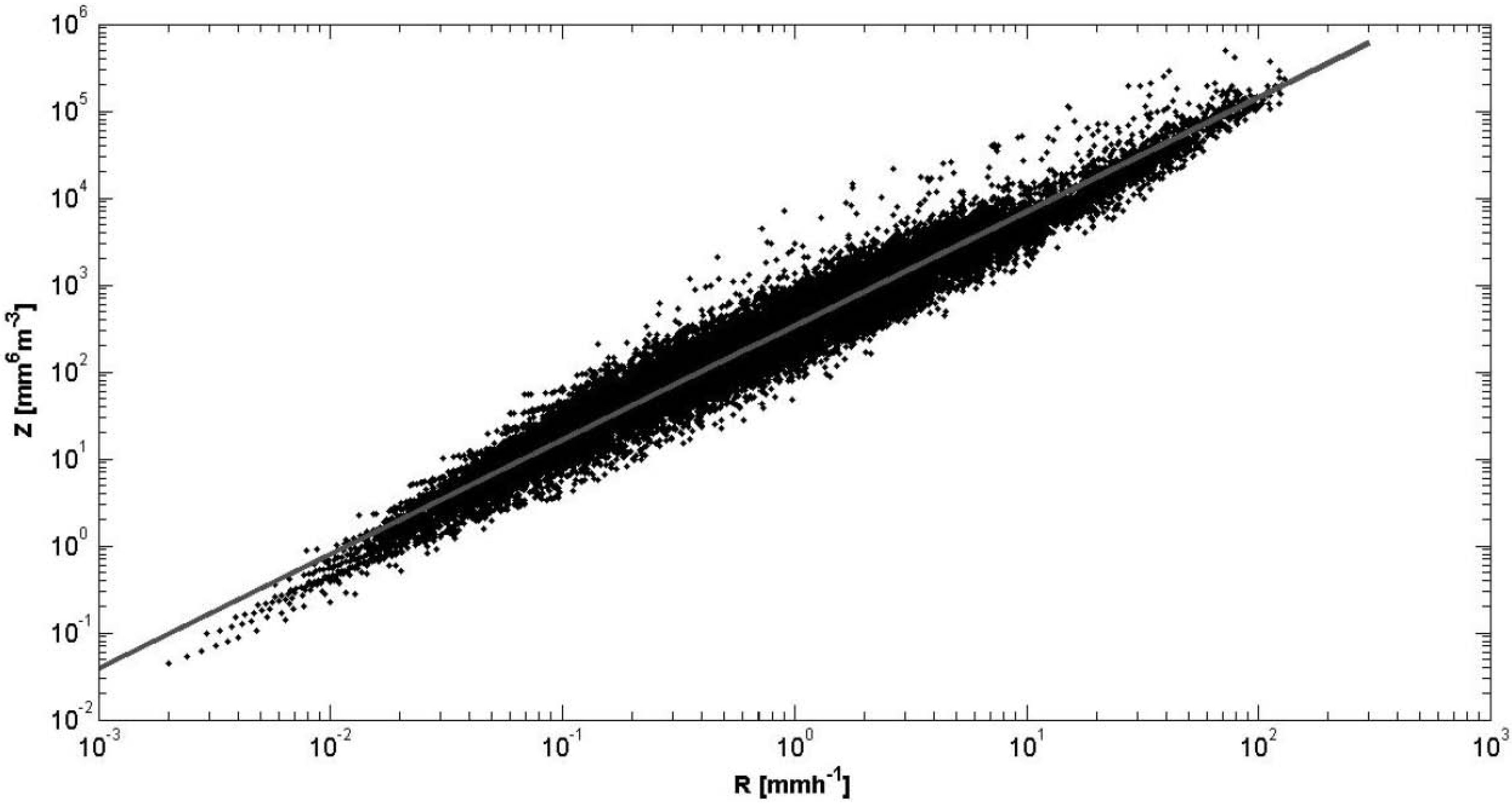
The use of only one relationship cannot generally represent the natural variability of precipitations. For example (see Figure 1), for a value of R, one can get several values corresponding to Z and vice versa.

Several studies have been conducted for the modelling of the size of rain drops under different latitudes [13]. The theoretical distribution functions evaluated are many but likely are not easy to manipulate [6]. The disdrometer allows measuring automatically and continuously the extent of rain drop distribution.

In this study, we want to adapt the neural network technique to the Rain Drop Size Distribution (RDSD) of precipitations in order to conceive a model which could take into account the distinct types of rain perturbations under different latitudes, with the RDSD. The liquid water content (M), the rain rate (R) and the radar reflectivity (Z) are considered as outputs.

The most important property of the neural networks is the nature of their adaptation, which may be deducted from samples. This characteristic provides some tools, which are able to solve high non-linear relationships [14]. The neural network is an alternative tool for modelling and describing complex relationships between physical or technical parameters [15]. It is considered as an “engine” delivering to its entries an “answer” which is inaccessible or not easily accessible with existing analytical methods. In the following work, we describe briefly the theory of neural networks, presenting the Feed Forward Back Propagation (FFBP) and the Cascade Forward Back Propagation (CFBP) models. We will then situate the five African localities which were subject to our experimental work and where the collection and the classification of the rain drops were realized, while using the disdrometer. Lastly, we will describe how the different neural network models have been constructed, trained and used for the estimation of the water content, the rain rate and the radar reflectivity. We present the results in the form of curve comparisons and calculated root means square errors (RMSE).

Figure 1. Radar reflectivity factor Z vs. rain rate R as deduced from the 1-min rain RDSD (Rain Drop Size Distribution) observed with the JWD (Joss-Waldvogel Disdrometer) in Dakar (Senegal), during 1997–2002, and fitted curve.

Figure 1. Radar reflectivity factor Z vs. rain rate R as deduced from the 1-min rain RDSD (Rain Drop Size Distribution) observed with the JWD (Joss-Waldvogel Disdrometer) in Dakar (Senegal), during 1997–2002, and fitted curve.

2. Theoretical Background on Artificial Neural Networks

2.1. Basic Principles

An artificial neural network is organized into several layers. One layer contains some neurons which are connected to those of the following layer. Each connection is weighed. A neuron is described with its own activation level, which is responsible for the propagation of the information from the input layer to the output layer. However, to obtain reliable weights, the neural network must, first of all, learn about the known input- and output-samples. During the learning process, an error between theoretical and experimental outputs is computed. Thus, the weight-values are modified through an error back propagation process which is executed on several sampling data, until achieving as small error as possible. After this last step, the neural network can be considered as trained and able to be used in calculating other responses to new entries that have never been presented to the network. It is important to emphasize that the learning speed of the neural network depends not only on the architecture but also on the algorithm used.

2.2. Model of a Neuron in a Neural Network

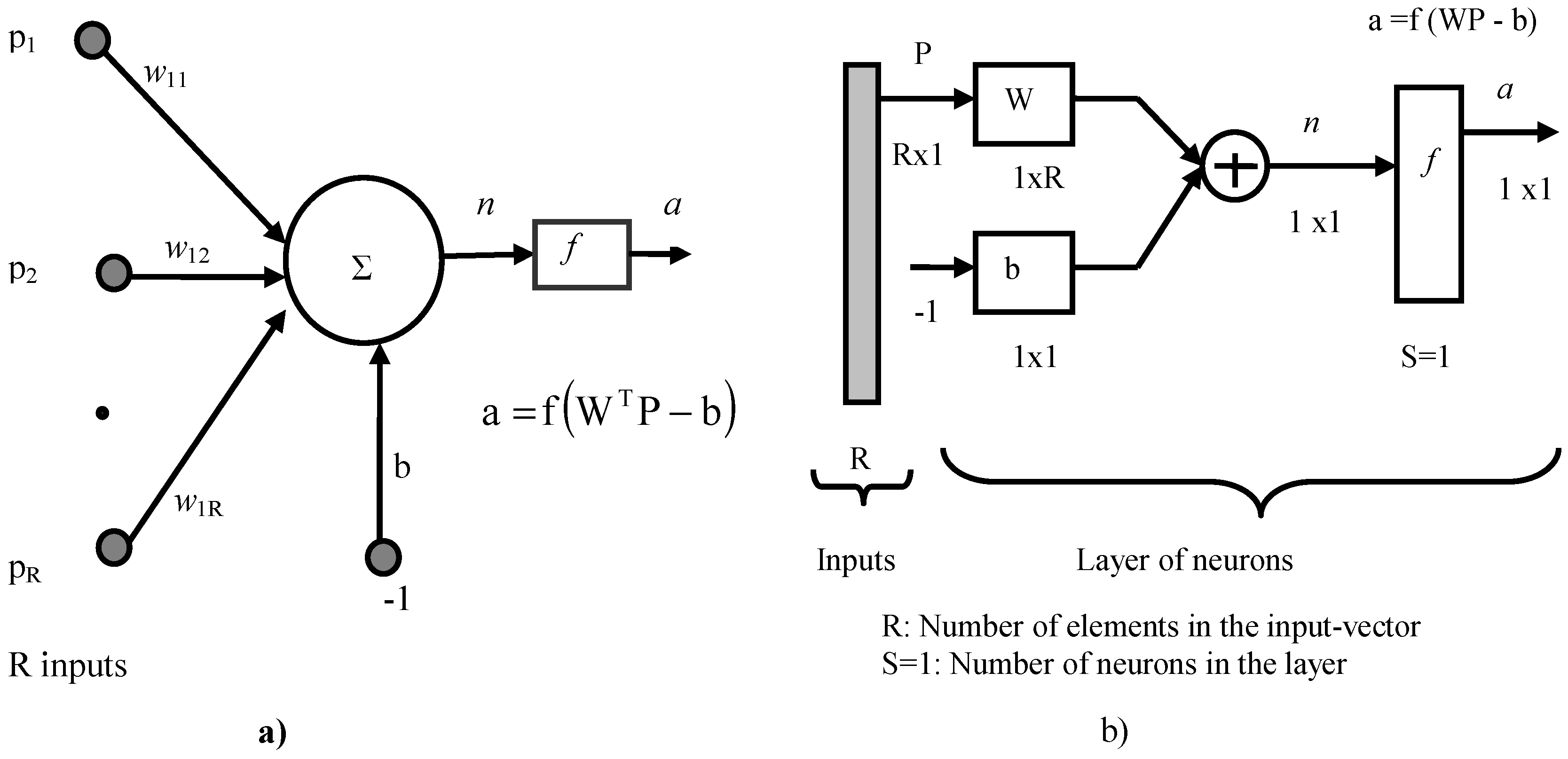
The neuron is considered as an elementary cell in which some computational operations are realized (see Figure 2a). It is composed of an integrator (∑) which calculates the weighted sum of the entries. The activation level n, with b as bias, of this integrator, is transformed by a transfer function f in order to produce an output a. The matrix representation of the neuron is shown on Figure 2b, with S supposed to be equal to the unity, to signify that there is only one neuron [16].

Figure 2. Representation of a neuron: (a) model; (b) matrix representation for S = 1.

Figure 2. Representation of a neuron: (a) model; (b) matrix representation for S = 1.

The R entries of the neuron correspond to the vector P = [P₁ P₂ … P_R]^T while W = [W₁₁ W₁₂ … W_1R]^T represents the vector weights of the neuron. The output n of the integrator is then described by Equation (1):

(1)

If the argument of the function f becomes zero or positive, the activation level reaches or is superior to the bias b, if not, it is negative [16,17].

The output of the neuron is given by the Equation (2):

a = f (n) = f (W^T P − b)

(2)

2.3. Construction of a Neural Network and its Learning Process

To build a neural network, it is sufficient to combine the neural layers. Each layer has its own matrix weight W^k, where k designates the index of the layer. Thus, the vectors b^k, n^k and a^k are associated to the layer k. To specify the neural network structure, the number of layers and the number of neurons in each layer must be chosen. The learning step is a dynamic and iterative process which consists in modifying the parameters of the network after receiving the inputs from its environment. The learning type is determined by the way the change of the parameters occurs [14]. In almost all neural architectures encountered, the learning results in the synaptic modification of the weights connecting one neuron to the other. If w_ij (t) designates the weight connecting the neuron i to its entry j and at time t, a change ∆w_ij (t) of the weights can simply be expressed by the Equation (3):

∆w_ij (t) = w_ij (t + 1) − w_ij (t)

(3)

where w_ij (t + 1) represents the new entry value of the weight w_ij.

A set of well-defined rules that allow realizing a weight adaptation process is designated by a learning algorithm of the neural network. There are a lot of rules that can be used. We can enumerate among others: the method of learning by error correction, the so-called Least Mean Square (LMS) method; the feed forward back propagation in a multilayer neural network; and the method of the back propagation of error sensitivities. In our study, we focalize on the method based on a small modification of the feed forward back propagation method.

2.4. The Feed Forward Back Propagation Method Used by a Multilayer Neural Network

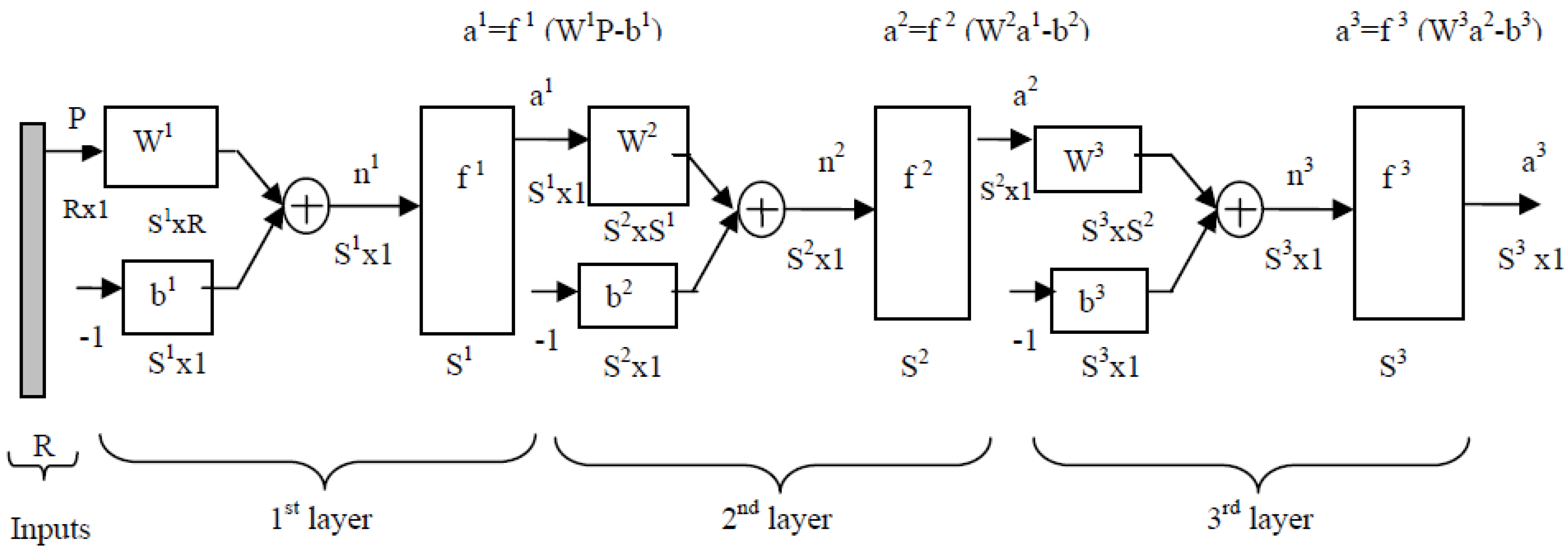
Let us now consider the multilayer neural network (composed of M layers) whose synoptic graphical representation is given in Figure 3 for three layers. The equation describing the outputs of the layer k is:

a^k = f ^k [W^k a^{k −1} − b^k], k = 1, …, M

(4)

In the presence of sample-data combinations entries/outputs{(P_q, d_q)}, q = 1, …, Q, where P_q designates an entry-vector and d_q a desired output-vectors, we can forward propagate at each instant t, an entry-vector P(t) through the neural network in order to get an output-vector a(t).

Figure 3. An example of synoptic representation of a 3 layer-neural network in a feed forward back propagation form.

Figure 3. An example of synoptic representation of a 3 layer-neural network in a feed forward back propagation form.

Given here are e(t), the error produced by the network calculation for an entry, and the corresponding desired output d(t):

e (t) = d (t) − a (t)

(5)

The performance function F that permits minimizing the root mean square error is defined by the following expression:

F(X) = E[e^T (t) · e (t)]

(6)

where E[ ] and X are respectively the mean and the vector grouping the set of the weights and the biases of the neural network. F will be approximated on a layer with the instantaneous error:

(7)

The method of the steepest falling gradient is used to optimize X with the help of the following equations:

(8)

where η designates the learning rate of the neural network. To calculate the partial derivatives of the rule of composition functions is used:

(9)

The activation levels of the layer k depend directly on the weights and biases on this layer, and can be expressed by the following relation:

(10)

Now, for the first terms of the Equation (9), we define the sensitivities of in relation with the changes of the activation level of the neuron i belonging to the layer k by the equation:

(11)

The expressions of and become:

(12)

Equation (12) is responsible for the modification of the weight connections and biases and the different iteration learning steps of the neural network presented in Section 4.

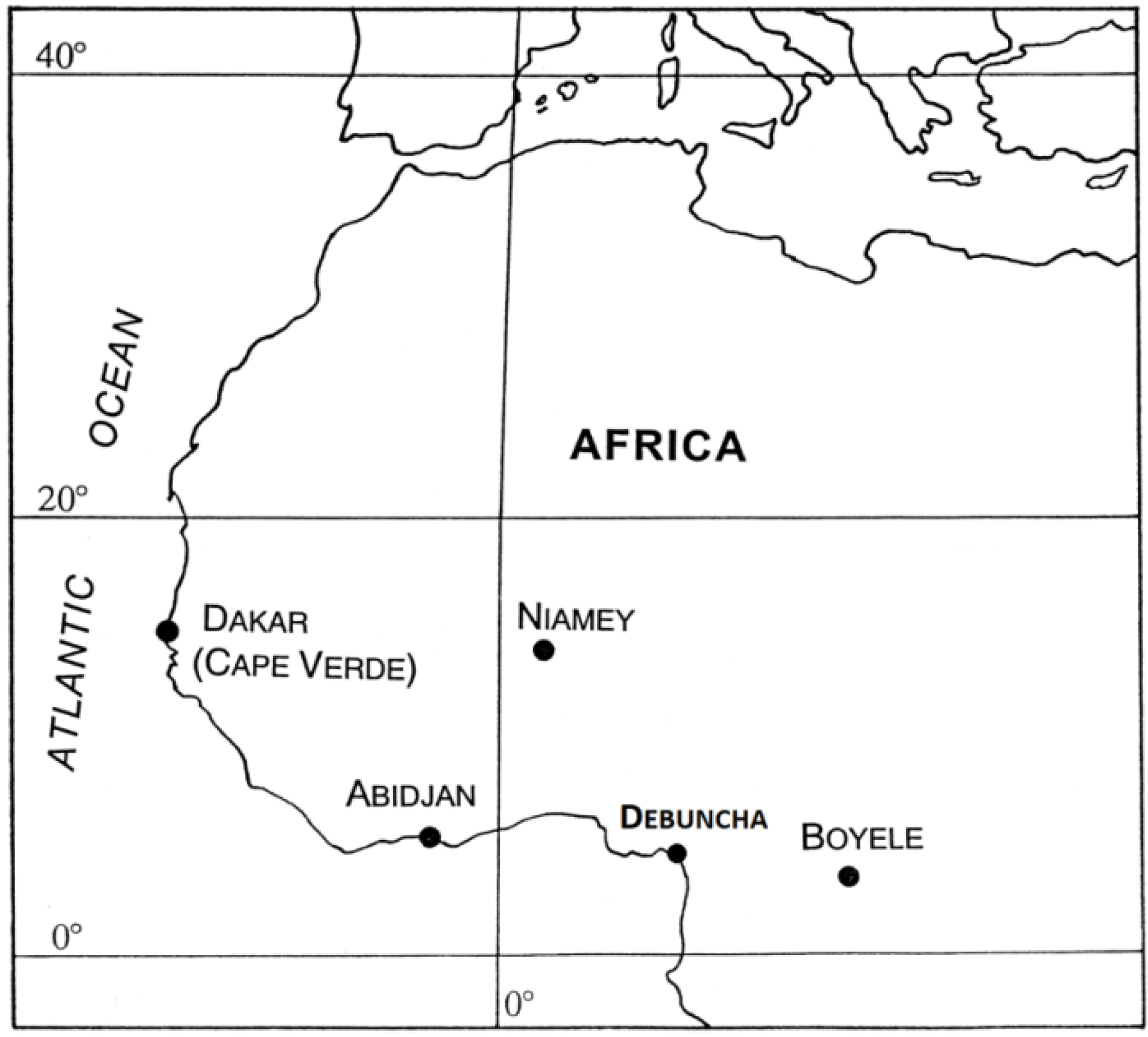
3. Localities and Data Used for the Study

The applications of our study have been realized after using the RDSD. These data have been collected under different latitudes in Sub-Saharan Africa (see Figure 4). Their main characteristics are grouped in the Table 1. The disdrometer used for the data collection is a mechanical one and was developed by Joss and Waldvogel [18,19]. This instrument produces the RDSD minute by minute. The technical description of its functions is given by [18,19,20,21].

The principle of data processing of the disdrometer consists in classifying repeatedly in an interval of one minute the rain drops according to their diameter. During the collection period, some values are computed with the data by minute in order to obtain the values of some rain parameters such as the total number of rain drops, the distribution of the rain drop size, the rain rate, the radar reflectivity, the liquid water content and the median volume diameter.

Figure 4. Location of the data collection sites.

Figure 4. Location of the data collection sites.

Table 1. Database and localities studied in sub-Saharan Africa.

Town (Country)	Collection Period of the RDSD	Total Number of the RDSD (min)
Abidjan (Ivory Coast)	June; September to December: 1986	23,126
Boyele (Congo)	March to June: 1989	18,354
Debuncha (Cameroon)	May to June 2004	39,113
Dakar (Senegal)	July to September: 1997, 1998 et 2000	15,145
Niamey (Niger)	July to September: 1989	4468

Table 1. Database and localities studied in sub-Saharan Africa.

Town (Country)	Collection Period of the RDSD	Total Number of the RDSD (min)
Abidjan (Ivory Coast)	June; September to December: 1986	23,126
Boyele (Congo)	March to June: 1989	18,354
Debuncha (Cameroon)	May to June 2004	39,113
Dakar (Senegal)	July to September: 1997, 1998 et 2000	15,145
Niamey (Niger)	July to September: 1989	4468

Table 2. Values of the exponent factor p and of the multiplicative factor a_p in relation to the parameter studied ( ).

Parameter	Symbol P	Exponent Factor p	Unit	Multiplicative Factor ap
Rain rate	R	3.67	mm∙h−1	7.1 × 10−3
Liquid water content	W	3	g∙m−3	(π/6) × 10−3
Radar reflectivity factor	Z	6	mm6∙m−3	1

Table 2. Values of the exponent factor p and of the multiplicative factor a_p in relation to the parameter studied ( ).

Parameter	Symbol P	Exponent Factor p	Unit	Multiplicative Factor ap
Rain rate	R	3.67	mm∙h−1	7.1 × 10−3
Liquid water content	W	3	g∙m−3	(π/6) × 10−3
Radar reflectivity factor	Z	6	mm6∙m−3	1

The control parameters of the RDSD are calculated by different drop-diameter moments observed [10] and changes with particular used moments [22,23,24,25,26]. The parameters M, R and Z exploited in our study can be expressed in a generic form as follows:

(13)

where N(D) is the number of rain drops per unit height and per volume (mm⁻¹∙m⁻³), D (mm) is the diameter of the equivalent sphere, and a_P a coefficient which depends on the type of parameter considered and on the chosen units, so as shown in t Table 2. The stated disdrometer observation normally has large errors for small drop size and large drop size [27]. The coefficient p in Equation (13) is issued from the definition of the parameters; Z and R are respectively defined as the moment of order 6 and 3.67 of the diameter D [28].

4. Methodology

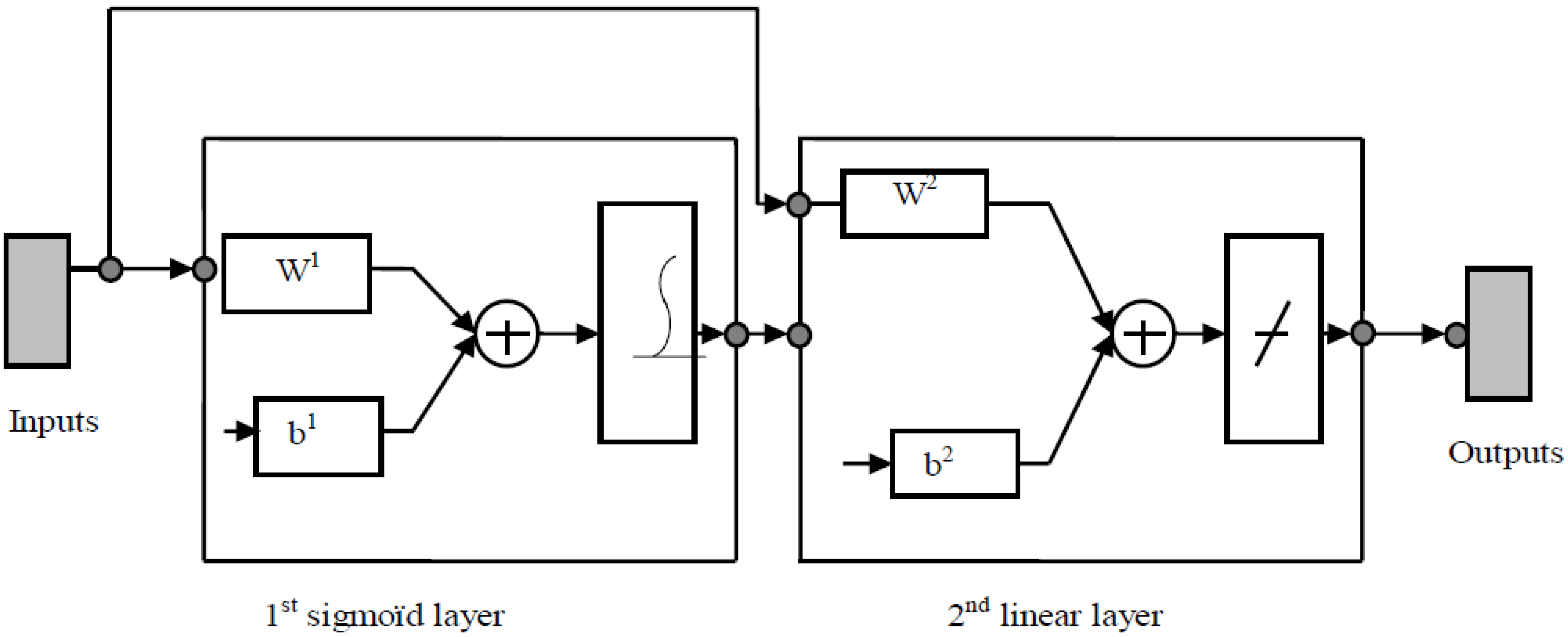
The modelling process of a neural network requires the disposal of an entry’s number R as well as the number of neurons in the output layer. These neural networks are defined by the specifications of the problem to be solved. The CFBP (Cascade Forward Back Propagation) model (see Figure 5) is one of the artificial neural network types, which is used for the prediction of new output data [29,30,31].

Figure 5. Model of Cascade Forward Back Propagation (CFBP).

Figure 5. Model of Cascade Forward Back Propagation (CFBP).

Taking into consideration the different analyses in, we will give an abstract of the methodology used in the learning process that we have implemented.

• Initialize the weights with small random values;
• For each combination (p_q, d_q) in the learning sample:

  • Propagate the entries p_q forward through the neural network layers:

    a⁰ = p_q; a^k = f ^k (W ^k a^{k −1} − b^k), k = 1, …, M

    (14)
  • Back propagate the sensitivities through the neural network layers:

    δ^M = −2F^′M (n^M) (d_q − a^M); δ^k = F^′k (n^k) (W^{k +1})^T δ^k+1, k = M − 1, …, 1

    (15)
  • Modify the weights and biases:

    ∆W^k = −η δ^k(a^{k −1})^T, k = 1, …, M,
    ∆b^k = η δ^k, k = 1, …, M

    (16)
• If the stopping criteria are reached, then stop; if not reached, they permute the presentation order of the combination built from the learning database, and begin again at Step 2.

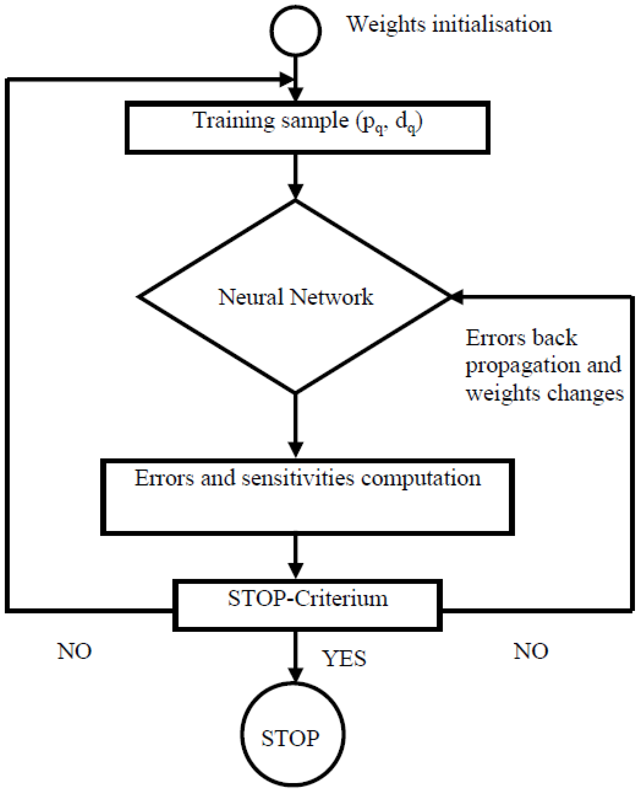
The diagram describing the different steps of the learning process of the neural network is given by Figure 6.

Figure 6. Diagram of the learning process of the neural network.

Figure 6. Diagram of the learning process of the neural network.

4.1. Description of the Databases and their Use in the Neural Models

The classes of diameters are used as entries of the neural network models in order to estimate the water content, the rain rate and the radar reflectivity factor. Thus, the neural networks will then be constituted of 25 entries corresponding to the 25 classes and of one output. The samples presented to the entry of the neural network correspond each to the one-minute values that were calculated by the disdrometer.

On the basis of the retrieval work, we then have two databases that we have named as “Base X” and “Base Y”. They are each made up of 23,126 samples. Each sample from the first database is a vector of 25 elements X[x₁, x₂, …, x₂₅]^T. The base Y is a matrix of 23,126 × 3 dimensions whose three rows represent three different vectors, Y₁, Y₂ and Y₃. These three last vectors are known as the water content (M(g∙m⁻³)), the rain rate (R(mm∙h⁻¹)) and the radar reflectivity (Z(mm⁶∙m⁻³)), each retrievable individually, from the X database. With each sample j of the first database is then associated a real number y_ij(i = 1,2,3; j = 1,2,…,23126). In this work, we have to retrieve these parameters. 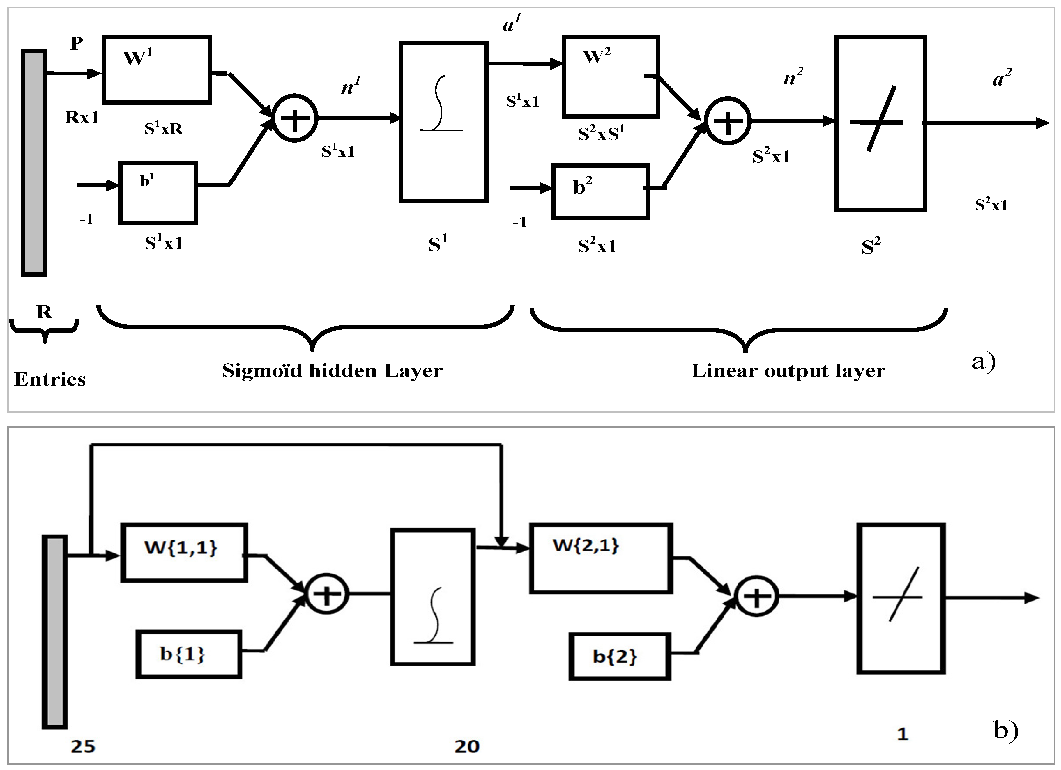The different neural networks have as entries the parameters x_k (k = 1,2,…,25) and as outputs the parameter y_i (i = 1,2,3). The neural model is a cascade forward back propagation (CFBP) one, with a hidden layer of 20 neurons (Figure 7a,b). We develop for each locality a model which will be applied to other localities before building another model, which will integrate all five localities. This last model will be applied on all five localities.

Figure 7. ANN models: (a) description of the model; (b) the faster CFBP model, which was used for our simulations.

Figure 7. ANN models: (a) description of the model; (b) the faster CFBP model, which was used for our simulations.

-

R entry’s number (25 in our case)

-

S1: Number of neurons in the first layer (hidden layer): 20 in our case

-

S2: Number of neurons in the output layer: 1 in our case

-

b1: Bias’ vector of the first layer with the dimension S¹ × 1 (20 × 1 dimension in our case)

-

b2: Bias’ vector of the output layer with the dimension S² × 1 (1 × 1 in our case)

-

W1: Matrix of weights according to the neurons of the first layer with the dimension S¹ × R (20 × 25 dimension in our case);

-

W2: Matrix of weights according to the neurons of output layer with the dimension S² × S¹ (1 × 20 dimension in our case)

4.2. Construction and Use of the Different Neural Networks

The databases are available for five studied localities, and two approaches are taken into consideration:

First, we create for each locality three LANN-models corresponding to the three parameters y_i. The initial 5000 entries and the primary 5000 desired outputs, except Niamey with only 4468 sample data, are used for the training of the neural networks, and the 5000 following sample data (from the 5001st to 10,000th) have served as test data. After the training, we have obtained acceptable performance curves and have stored the LANN, that we designate by the indices, i, to confer them the role of retrieving the parameter y_i. Each LANN i of a given locality is then invited to predict the parameters y_i over the other localities. In this case, we have used as LANN inputs the entries obtained in the locality subjected to the predictive process. We estimate for the samples from the 5001st–10,000th the outputs that we compare with the available experiment present in this locality.

Secondly, we build for each parameter Y_i(M, R, Z) a polyvalent model (PANN): we extract from the databases of each locality the first 1200 sample data and constitute a training set composed of 6000 training data combinations. Each PANN i (i indicating its role of retrieval of parameter Y_i) is then used to predict the parameters Y_i over all localities. As follows, we use the designations from Table 3 and the notations M, R and Z, respectively, for the variables Y1, Y2 and Y3.

Table 3. Model designation for each locality.

Locality	Neural Model Developed by Data from the Locality
Abidjan (Ivory Coast)	A
Boyele (Congo Brazzaville)	B
Debuncha (Cameroon)	C
Dakar (Senegal)	D
Niamey (Niger)	N
All localities	PANN

Table 3. Model designation for each locality.

Locality	Neural Model Developed by Data from the Locality
Abidjan (Ivory Coast)	A
Boyele (Congo Brazzaville)	B
Debuncha (Cameroon)	C
Dakar (Senegal)	D
Niamey (Niger)	N
All localities	PANN

5. Results and Discussions

5.1. Capability of a Neural Network to Estimate the Parameters in Various Other Localities

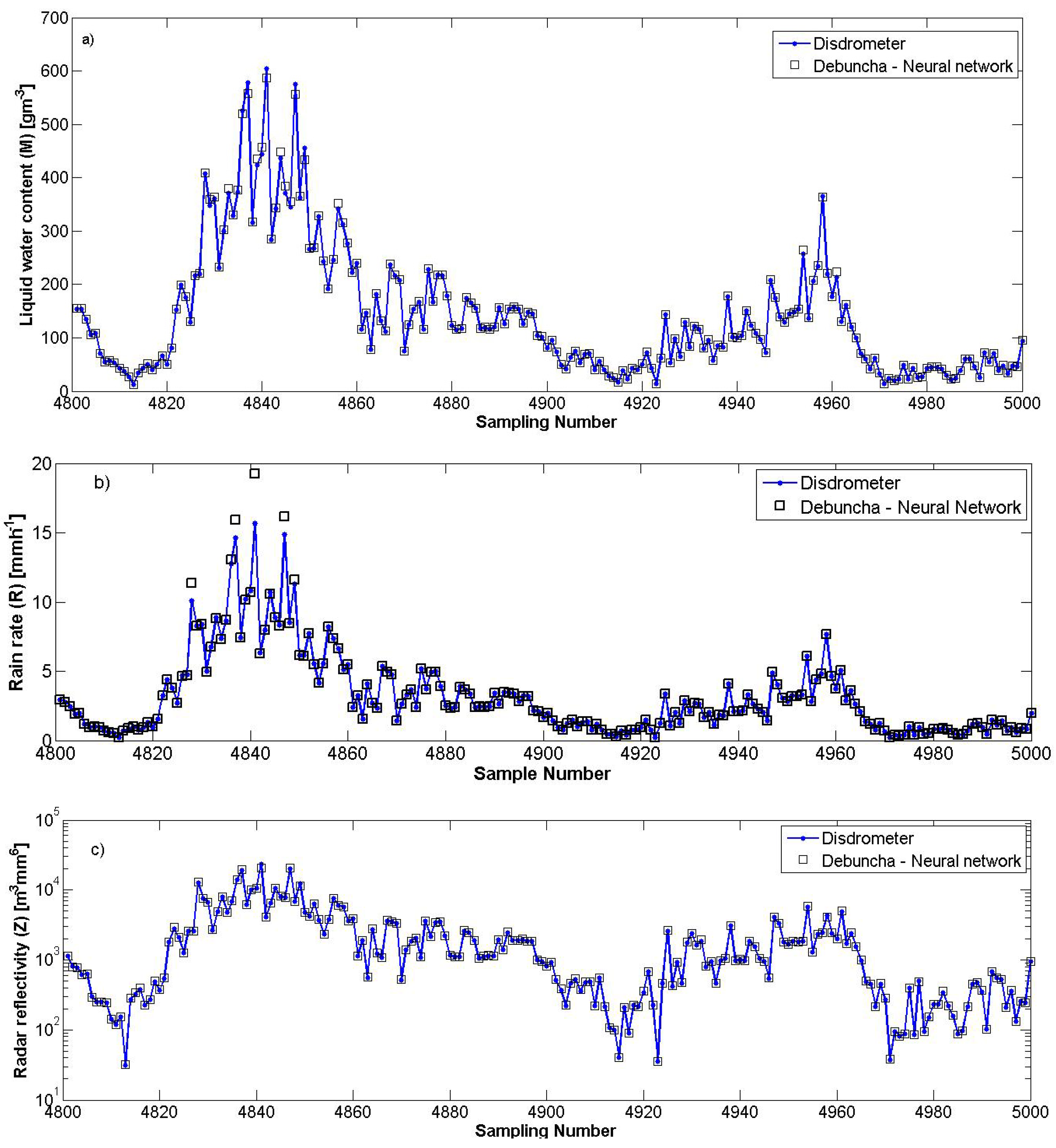
We have estimated the values of the three parameters (M, R and Z) over five localities with a LANN which has been trained only with the experimental RDSD values measured in Debuncha (Cameroon). For example, after using the first 500 training samples of this locality, we predicted in Abidjan (Côte d’Ivoire) 200 values for each parameter, corresponding to the sample data from the 4801st to the 5000th and have obtained the approximations presented in Figure 8. The dots correspond to the experimental values and the squares to the estimated ones.

The different approximations can be considered as very good because the values measured by the disdrometer are practically the same as those estimated by the LANN.

5.2. Estimation of the Values of M, R and Z with the PANN

We have shown that a LANN which has been trained with disdrometer parameters issued only from a given locality, in order to estimate the parameters M, R and Z, was also able to estimate the same parameters in another locality, which is far different from the first. For ameliorating this type of estimation, we have created another ANN that we have qualified as a polyvalent one (PANN) and, which takes into account, while it is in development, data issued from all the localities where it will be used for prediction. For our concrete case, we have put together the first 1200 sampling data of each locality in order to obtain training values. The trained PANN has been used to estimate 5000 values of M, R and Z over all five localities, namely those from the 1201st to the 6200th.

Figure 8. Neural prediction in Abidjan (Ivory Coast) of the liquid water content M (a), the rain rate R (b) and the radar reflectivity Z (c) by a LANN constructed with data issued only from Debuncha (Cameroon).

Figure 8. Neural prediction in Abidjan (Ivory Coast) of the liquid water content M (a), the rain rate R (b) and the radar reflectivity Z (c) by a LANN constructed with data issued only from Debuncha (Cameroon).

5.3. Evaluation of the Root Mean Square Errors (RMSE)

We have evaluated the root mean square errors produced by the LANN and the PANN estimation, while comparing the estimates to the disdrometer measures. Equation (17) has been used:

(17)

where E_i: Error (observed value−Neural Network estimate); and N: Number of observed values.

5.3.1. RMSE between Measured Parameters in the Localities and Estimates Delivered by the LANN A, B, C, D and N

We present in Table 4 the RMSE between values measured by the disdrometer and those estimated by the different LANN.

If the estimates over a given locality are delivered by a LANN trained with data issued from another locality, N is equal to 5000 (except the estimations realized in Niamey (Niger), only 4468 values were available). The estimations produced locally by the LANN concern the sample data from the 5001st to the 10,000th.

Table 4. Comparisons between RMSE after use of the different LANN (A, B, C, D and N).

LANN	Abidjan			Boyele				Debuncha
	Y1 (M)	Y2 (R)	Y3 (Z)	Y1 (M)		Y2 (R)	Y3 (Z)	Y1 (M)	Y2 (R)	Y3 (Z)
A	0.01	0.01	0.58	4.87		0.35	870.16	17.60	1.25	3144.06
B	0.04	0.14	1.27	0.01		0.01	0.24	0.02	0.03	0.58
C	0.02	0.06	1.05	0.01		0.01	0.49	0.01	0.01	0.33
D	0.83	0.15	1.91	0.17		0.01	0.36	0.48	0.06	0.66
N	0.07	0.54	3.77	0.01		0.01	0.46	0.03	0.13	0.83
LANN	Dakar							Niamey
	Y1 (M)		Y2 (R)		Y3 (Z)			Y1 (M)	Y2 (R)	Y3 (Z)
A	6.11		0.44		1091.45			3.57	0.26	638.14
B	0.01		0.01		0.35			0.01	0.01	0.25
C	0.01		0.01		0.62			0.01	0.01	0.45
D	0.01		0.01		0.15			0.13	0.01	0.22
N	0.02		0.02		0.38			0.01	0.01	0.13

Table 4. Comparisons between RMSE after use of the different LANN (A, B, C, D and N).

LANN	Abidjan			Boyele				Debuncha
	Y1 (M)	Y2 (R)	Y3 (Z)	Y1 (M)		Y2 (R)	Y3 (Z)	Y1 (M)	Y2 (R)	Y3 (Z)
A	0.01	0.01	0.58	4.87		0.35	870.16	17.60	1.25	3144.06
B	0.04	0.14	1.27	0.01		0.01	0.24	0.02	0.03	0.58
C	0.02	0.06	1.05	0.01		0.01	0.49	0.01	0.01	0.33
D	0.83	0.15	1.91	0.17		0.01	0.36	0.48	0.06	0.66
N	0.07	0.54	3.77	0.01		0.01	0.46	0.03	0.13	0.83
LANN	Dakar							Niamey
	Y1 (M)		Y2 (R)		Y3 (Z)			Y1 (M)	Y2 (R)	Y3 (Z)
A	6.11		0.44		1091.45			3.57	0.26	638.14
B	0.01		0.01		0.35			0.01	0.01	0.25
C	0.01		0.01		0.62			0.01	0.01	0.45
D	0.01		0.01		0.15			0.13	0.01	0.22
N	0.02		0.02		0.38			0.01	0.01	0.13

Table 5 gives the two best LANN for the retrieval of the parameters M, R and Z.

Table 5. Choice of the two best LANN for retrieval of the parameters in the different localities (A, B, C, D and N).

	Abidjan		Boyele		Debuncha		Dakar		Niamey
	1st	2nd	1st	2nd	1st	2nd	1st	2nd	1st	2nd
	LANN	LANN	LANN	LANN	LANN	LANN	LANN	LANN	LANN	LANN
M	A	C	B	C	C	B	D	C	N	C
R	A	C	B	D	C	B	D	C	N	B
Z	A	C	B	D	C	B	D	B	N	D

Table 5. Choice of the two best LANN for retrieval of the parameters in the different localities (A, B, C, D and N).

	Abidjan		Boyele		Debuncha		Dakar		Niamey
	1st	2nd	1st	2nd	1st	2nd	1st	2nd	1st	2nd
	LANN	LANN	LANN	LANN	LANN	LANN	LANN	LANN	LANN	LANN
M	A	C	B	C	C	B	D	C	N	C
R	A	C	B	D	C	B	D	C	N	B
Z	A	C	B	D	C	B	D	B	N	D

Considering the results obtained in Table 4 and Table 5, we observe that the best LANN for the estimation in a locality is logically the one which has been developed with data issued from that same locality and shows that the LANN of Debuncha (Cameroon) is in almost all cases able to predict the parameters in other localities.

5.3.2. RMSE between Values Measured by the Disdrometer and Estimates Delivered by the PANN

We have constructed a polyvalent ANN model (PANN) with data issued from the five localities and have chosen the data-gathering order: A+B+C+D+N. The training entries and the desired outputs are constituted by the first 1200 sampling data from A, the initial 1200 sampling data from B, the primary 1200 sampling data from C, the initial 1200 sampling data from D and lastly, the first 1200 sampling data from N. We have calculated and presented in Table 6 the RMSE between values measured by the disdrometer and those estimated by the PANN.

Table 6. RMSE between values measured by the disdrometer and those estimated by the PANN.

Abidjan				Boyele					Debuncha
M	R		Z	M		R		Z	M		R		Z
0.02	0.01		0.66	0.01		0.01		0.24	0.02		0.01		0.52
Dakar							Niamey
M		R			Z		M			R		Z
0.01		0.01			0.25		0.01			0.01		0.15

Table 6. RMSE between values measured by the disdrometer and those estimated by the PANN.

Abidjan				Boyele					Debuncha
M	R		Z	M		R		Z	M		R		Z
0.02	0.01		0.66	0.01		0.01		0.24	0.02		0.01		0.52
Dakar							Niamey
M		R			Z		M			R		Z
0.01		0.01			0.25		0.01			0.01		0.15

Observing the results obtained, the use of the PANN allows obtaining the best RMSE-values (Table 6). However, it is to be noted that while juxtaposing the training data, the order of the localities must be also respected in the fusion of the desired outputs.

Table 7. Comparisons between RMSE after use of the different LANN: Case of stratiform rains.

LANN	Abidjan				Boyele						Debuncha
	Y1 (M)	Y2 (R)		Y3 (Z)	Y1 (M)		Y2 (R)		Y3 (Z)		Y1 (M)	Y2 (R)		Y3 (Z)
A	0.010	0.010		0.130	0.940		0.052		67.49		1.730	0.125		118.5
B	0.010	0.010		0.075	0.010		0.010		0.043		0.010	0.010		0.063
C	0.010	0.010		0.130	0.010		0.010		0.098		0.010	0.010		0.075
D	0.010	0.010		0.100	0.015		0.010		0.089		0.010	0.061		0.360
N	0.020	0.010		0.092	0.010		0.010		0.066		0.012	0.058		0.220
LANN	Dakar							Niamey
	Y1 (M)		Y2 (R)			Y3 (Z)		Y1 (M)		Y2 (R)			Y3 (Z)
A	1.100		0.074			52.45		1.450		0.089			124.0
B	0.010		0.010			0.051		0.010		0.010			0.058
C	0.010		0.010			0.120		0.010		0.010			0.120
D	0.010		0.010			0.060		0.010		0.010			0.070
N	0.010		0.010			0.110		0.010		0.010			0.05

Table 7. Comparisons between RMSE after use of the different LANN: Case of stratiform rains.

LANN	Abidjan				Boyele						Debuncha
	Y1 (M)	Y2 (R)		Y3 (Z)	Y1 (M)		Y2 (R)		Y3 (Z)		Y1 (M)	Y2 (R)		Y3 (Z)
A	0.010	0.010		0.130	0.940		0.052		67.49		1.730	0.125		118.5
B	0.010	0.010		0.075	0.010		0.010		0.043		0.010	0.010		0.063
C	0.010	0.010		0.130	0.010		0.010		0.098		0.010	0.010		0.075
D	0.010	0.010		0.100	0.015		0.010		0.089		0.010	0.061		0.360
N	0.020	0.010		0.092	0.010		0.010		0.066		0.012	0.058		0.220
LANN	Dakar							Niamey
	Y1 (M)		Y2 (R)			Y3 (Z)		Y1 (M)		Y2 (R)			Y3 (Z)
A	1.100		0.074			52.45		1.450		0.089			124.0
B	0.010		0.010			0.051		0.010		0.010			0.058
C	0.010		0.010			0.120		0.010		0.010			0.120
D	0.010		0.010			0.060		0.010		0.010			0.070
N	0.010		0.010			0.110		0.010		0.010			0.05

5.3.3. Computation of the RMSE after Distinction of Stratiform and Convective Rains

The RMSE calculated and presented in Table 4 and Table 6 concern generally rainfall without a distinction between stratiform and convective rains. This has led us to obtain very small RMSE values. The differentiation between these two rains types enable understanding the importance of the different contributions brought by the two types during the rain period. For this purpose, we have constituted two value classes: the first database corresponds to the values M < 410, R < 10, Z < 10,810 (stratiform situation), and the second database corresponds to the values M ≥ 410, R ≥ 10, Z ≥ 10,810 (convective situation). A separate evaluation of the RMSE gives the results presented in Table 7, Table 8, Table 9 and Table 10.

• Stratiform Rainfall

Table 7 gives the RMSE produced by the five LANN while estimating the parameters over all five localities. Here, only the stratiform rain is considered.

Table 8 presents the RMSE produced by the PANN in the five localities. Here, only the stratiform situation is considered.

Table 8. RMSE between values measured by the disdrometer and those estimated by the PANN: Case of the stratiform rains.

Abidjan				Boyele						Debuncha
M	R		Z	M		R		Z		M	R		Z
0.010	0.010		0.065	0.010		0.010		0.060		0.010	0.010		0.016
Dakar							Niamey
M		R			Z		M		R			Z
0.010		0.010			0.066		0.010		0.010			0.072

Table 8. RMSE between values measured by the disdrometer and those estimated by the PANN: Case of the stratiform rains.

Abidjan				Boyele						Debuncha
M	R		Z	M		R		Z		M	R		Z
0.010	0.010		0.065	0.010		0.010		0.060		0.010	0.010		0.016
Dakar							Niamey
M		R			Z		M		R			Z
0.010		0.010			0.066		0.010		0.010			0.072

Table 9. Comparisons between RMSE after using the different LANN: Case of the convective rainfall.

LANN	Abidjan				Boyele					Debuncha
	Y1 (M)	Y2 (R)		Y3 (Z)	Y1 (M)		Y2 (R)		Y3 (Z)	Y1 (M)		Y2 (R)		Y3 (Z)
A	0.011	0.010		0.140	13.91		1.030		2916.0	42.35		3.160		9009.7
B	0.076	0.310		3.040	0.020		0.015		0.7731	0.045		0.053		1.6500
C	0.030	0.130		2.510	0.015		0.020		1.6100	0.020		0.010		0.9500
D	1.670	0.316		4.610	0.480		0.010		1.150	0.480		0.010		1.6000
N	0.134	1.150		9.110	0.025		0.027		1.500	0.065		0.280		2.3000
LANN	Dakar							Niamey
	Y1 (M)		Y2 (R)			Y3 (Z)		Y1 (M)			Y2 (R)		Y3 (Z)
A	14.80		1.120			3410		10.17			0.760		2051.6
B	0.025		0.026			1.070		0.025			0.010		0.7700
C	0.020		0.017			1.890		0.020			0.010		1.4000
D	0.020		0.015			0.400		0.390			0.010		0.6700
N	0.040		0.187			1.130		0.014			0.012		0.3720

Table 9. Comparisons between RMSE after using the different LANN: Case of the convective rainfall.

LANN	Abidjan				Boyele					Debuncha
	Y1 (M)	Y2 (R)		Y3 (Z)	Y1 (M)		Y2 (R)		Y3 (Z)	Y1 (M)		Y2 (R)		Y3 (Z)
A	0.011	0.010		0.140	13.91		1.030		2916.0	42.35		3.160		9009.7
B	0.076	0.310		3.040	0.020		0.015		0.7731	0.045		0.053		1.6500
C	0.030	0.130		2.510	0.015		0.020		1.6100	0.020		0.010		0.9500
D	1.670	0.316		4.610	0.480		0.010		1.150	0.480		0.010		1.6000
N	0.134	1.150		9.110	0.025		0.027		1.500	0.065		0.280		2.3000
LANN	Dakar							Niamey
	Y1 (M)		Y2 (R)			Y3 (Z)		Y1 (M)			Y2 (R)		Y3 (Z)
A	14.80		1.120			3410		10.17			0.760		2051.6
B	0.025		0.026			1.070		0.025			0.010		0.7700
C	0.020		0.017			1.890		0.020			0.010		1.4000
D	0.020		0.015			0.400		0.390			0.010		0.6700
N	0.040		0.187			1.130		0.014			0.012		0.3720

Observing the results obtained in Table 7 and Table 8, we note that the RMSE, if considering only the stratiform situation, remains very small. This is proof that this rain type has been dominant during the rain period. Comparing Table 7 and Table 8, respectively, to Table 4 and Table 6, we can perceive that the values remain in the same level order.

• Convective Rainfall

We have only considered the data issued from the convective rainfall and calculated the RMSE produced by the LANN while estimating the parameters M, R and Z over each locality. Table 9 gives these errors for the five LANN and Table 10 presents them for the PANN.

Table 10. RMSE between values measured by the disdrometer and those estimated by the PANN: case of the convective rainfall.

Abidjan				Boyele					Debuncha
M	R		Z	M	R		Z		M	R		Z
0.022	0.020		1.600	0.020	0.010		0.770		0.030	0.010		1.420
Dakar						Niamey
M		R		Z		M		R			Z
0.020		0.010		0.750		0.020		0.010			0.420

Table 10. RMSE between values measured by the disdrometer and those estimated by the PANN: case of the convective rainfall.

Abidjan				Boyele					Debuncha
M	R		Z	M	R		Z		M	R		Z
0.022	0.020		1.600	0.020	0.010		0.770		0.030	0.010		1.420
Dakar						Niamey
M		R		Z		M		R			Z
0.020		0.010		0.750		0.020		0.010			0.420

Considering the results from Table 9 and Table 10, and comparing them respectively to Table 7 and Table 8, we observe that the RMSE concerning the convective situation is higher.

6. Conclusions

Our study concerns the estimation of water content (M), rain rate (R) and radar reflectivity (Z). For this purpose, we have used RDSD data measured by a disdrometer installed in five African sub-Saharan localities. We have developed and trained for each locality a LANN with the disdrometer data of the same locality and have used the trained LANN to estimate the parameters M, R and Z over all localities. We have also developed a polyvalent ANN model (PANN) whose training was realized with a combination of data issued from all the localities where it will be used for estimating the parameters over each locality.

We have, first of all, considered the precipitations generally before taking into account their stratiform and convective structures. For appreciating the capability of the developed and trained LANN and PANN to estimate the parameters, we have calculated the RMSE produced by them during their use over the distinct localities. Observing the different results and comparisons obtained, we have perceived that the PANN is very capable of predicting over all the localities the values of the parameter for which it has been developed.

The RMSE produced by the PANN, while considering stratiform structures, is generally lower than those induced while considering the convective ones. After our investigation, we can thus consider the LANN and the PANN as models, which are able to predict rainfall values under different latitudes.

In areas of low coverage measurement networks of meteorological parameters, as in our study area (sub-Saharan Africa), the implementation of a PANN in a chain of radar measurements for rainfall could provide better understanding and describe the precipitations independently of their form and locality of occurrence.

The neural network technique is known to be difficult to manipulate. However, the implementation of such a technique in modern data acquirement instruments like rain radars may constitute a very interesting method to be investigated. Putting in place such a technology could permit a simultaneous measurement of DSD and the computing of rain parameters.

In our future works, we will also conduct a sensitivity study that consists of evaluating the significance of the RMSE between disdrometer measurement, rain gauge observations and NN estimates taking into account the disdrometer errors caused by rain drop size limitation during the measurement process.

References

- Aires, F.; Prigent, C.; Rossow, W.B.; Rothstein, M. A new neural network approach including first guess for retrieval of atmospheric water vapour, cloud liquid water path, surface temperature, and emissivities over land from satellite microwave observations. J. Geophys. Res. 2001, 106, 14887–14907. [Google Scholar] [CrossRef]
- Kidd, C.; Levizzani, V. Status of satellite precipitation retrieval. Hydrol. Earth Syst. Sci. 2011, 15, 1109–1116. [Google Scholar] [CrossRef]
- Bouzeboudja, O.; Haddad, B.; Ameur, S. Estimation radar des précipitations par la méthode des aires fractionnelles. Larhyss J. 2010, 8, 7–26. [Google Scholar]
- Kumar, L.S.; Lee, Y.H.; Yeo, J.X.; Ong, J.T. Tropical rain classification and estimation of rain from Z-R (reflectivity-rain rate relationships) relationships. Prog. Electromagn. Res. B 2011, 32, 107–127. [Google Scholar] [CrossRef]
- Anagnostou, M.N.; Kalogiros, J.; Anagnostou, E.N.; Tarolli, M.; Papadopoulos, A.; Borga, M. Performance evaluation of high-resolution rainfall estimation by X-band dual-polarization radar for flash flood applications in mountainous basins. J. Hydrol. 2010, 394, 4–16. [Google Scholar] [CrossRef]
- Alfieri, L.; Claps, P.; Laio, F. Time-dependent Z-R relationships for estimating rainfall fields from radar measurements. Nat. Hazard. Earth Syst. Sci. 2010, 10, 149–158. [Google Scholar] [CrossRef]
- Marshall, J.S.; Palmer, W.M. The distribution of raindrops with size. J. Atmos. Sci. 1948, 5, 165–166. [Google Scholar]
- Battan, L.J. Radar Observations of the Atmosphere; University of Chicago Press: Chicago, IL, USA, 1973. [Google Scholar]
- Atlas, D.; Ulbrich, C.W.; Marks, F.D.; Amitai, E.; Williams, C.R. Systematic variation of drop size and radar-rainfall relations. J. Geophys. Res. 1999, 104, 6155–6169. [Google Scholar] [CrossRef]
- Tokay, A.; Short, D.A. Evidence from tropical raindrop spectra of the origin of rain from stratiform versus convective clouds. J. Appl. Meteorol. 1996, 35, 355–371. [Google Scholar] [CrossRef]
- Tokay, A.; Short, D.A.; Williams, C.R.; Ecklund, W.L.; Gage, K.S. Tropical rainfall associated with convective and stratiform clouds: Intercomparison of disdrometer and profiler measurements. J. Appl. Meteorol. 1999, 38, 302–320. [Google Scholar] [CrossRef]
- Maki, M.; Keenan, T.D.; Sasaki, Y.; Nakamura, K. Characteristics of the raindrop size distribution in tropical continental squall lines observed in Darwin, Australia. J. Appl. Meteorol. 2001, 40, 1393–1412. [Google Scholar] [CrossRef]
- Bumke, K.; Seltmann, J. Analysis of measured drop size spectra over land and sea. ISRN Meteorol. 2012. [Google Scholar] [CrossRef]
- Widrow, B.; Lehr, M.A. 30 years of adaptive neural networks: Perceptron, Madaline, and Backpropagation. Proc. IEEE 1990, 78, 1415–1442. [Google Scholar] [CrossRef]
- Malkeil Burton, G. A Random Walk down Wall Street; Norton & Company: New York, NY, USA, 1996. [Google Scholar]
- Parizeau, M. Réseaux de neurones, GIF-21140 et GIF-64326; Université Laval: Laval, QC, Canada, 2004. [Google Scholar]
- Shiguemori, E.H.; Haroldo, F.; da Silva, J.D.S.; Carvalho, J.C. Neural Network Based Models in the Inversion of Temperature Vertical Profiles from Radiation Data. In Proceedings of the Inverse Problem Design and Optimization (IPDO-2004) Symposium, Rio de Janeiro, Brazil, 17–19 March 2004.
- Joss, J.; Waldvogel, A. Ein spectrograph für niederschagstropfen mit automatisher auswertung (A spectrograph for the automatic analysis of raindrops). Pure Appl. Geophys. 1967, 68, 240–246. [Google Scholar] [CrossRef]
- Joss, J.; Waldvogel, A. Raindrop size distribution and sampling size errors. J. Atmos. Sci. 1969, 26, 566–569. [Google Scholar] [CrossRef]
- Sheppard, B.E.; Joe, P.I. Comparison of raindrop size distribution measurements by a Joss–Waldvogel disdrometer, a PMS 2DG spectrometer, and a POSS Doppler radar. J. Atmos. Ocean. Technol. 1994, 11, 874–887. [Google Scholar] [CrossRef]
- Tokay, A.; Kruger, A.; Krajewski, W.F. Comparison of drop size distribution measurements by impact and optical disdrometers. J. Appl. Meteorol. 2001, 40, 2083–2097. [Google Scholar] [CrossRef]
- Zhang, G.; Vivekanandan, J.; Brandes, E.; Menegini, R.; Kozu, T. The shape–slope relation in observed gamma raindrop size distributions: Statistical error or useful information? J. Atmos. Ocean. Technol. 2003, 20, 1106–1119. [Google Scholar] [CrossRef]
- Nzeukou, A.; Sauvageot, H.; Ochou, A.D.; Kebe, C.M.F. Raindrop size distribution and radar parameters at cape verde. J. Appl. Meteorol. 2004, 43, 90–105. [Google Scholar] [CrossRef]
- Smith, P.L.; Kliche, D.V. The bias in moment estimators for parameters of drop size distribution functions: Sampling from exponential distributions. J. Appl. Meteorol. 2005, 44, 1195–1205. [Google Scholar] [CrossRef]
- Cao, Q.; Zhang, G. Errors in estimating raindrop size distribution parameters employing disdrometer and simulated raindrop spectra. J. Appl. Meteor. Climatol. 2009, 48, 406–425. [Google Scholar] [CrossRef]
- Smith, P.L.; Liu, Z.; Joss, J. A study of sampling variability effects in raindrop size observations. J. Appl. Meteorol. 1993, 32, 1259–1269. [Google Scholar] [CrossRef]
- Cao, Q.; Zhang, G.; Brandes, E.; Schuur, T.; Ryzhkov, A.; Ikeda, K. Analysis of video disdrometer and polarimetric radar data to characterize rain microphysics in Oklahoma. J. Appl. Meteorol. Climatol. 2008, 47, 2238–2255. [Google Scholar] [CrossRef]
- Adrot, G.; Gosset, M.; Boudevillain, B.; Flaus, J.M. Inversion du Model d’observation d’un radar météorologique par une méthode ensembliste. e-STA 2008, 5, 29–34. [Google Scholar]
- Khatib, T.; Mohamed, A.; Sopian, K.; Mahmoud, M. Assessment of artificial neural networks for hourly solar radiation prediction. Int. J. Photoenergy 2012. [Google Scholar] [CrossRef]
- Omaima, N.; Al-Allaf, A. Cascade-Forward vs. Function Fitting Neural Network for Improving Image Quality and Learning Time in Image Compression System. In Proceedings of the World Congress on Engineering 2012 Vol II WCE 2012, London, UK, 4–6 July 2012.
- Dheeraj Badde1, S.; Gupta Anil, K.; Patki Vinayak, K. Cascade and feed forward back propagation artificial neural network models for prediction of compressive strength of ready mix concrete. IOSR J. Mech. Civ. Eng. 2012, 3, 1–6. [Google Scholar]
© 2014 by the authors; licensee MDPI, Basel, Switzerland. This article is an open access article distributed under the terms and conditions of the Creative Commons Attribution license (http://creativecommons.org/licenses/by/3.0/).
the rule of composition functions is used:
of the layer k depend directly on the weights and biases on this layer, and can be expressed by the following relation: