Article

Atmospheric Levels of Benzene and C1-C2 Carbonyls in San Nicolas de los Garza, Nuevo Leon, Mexico: Source Implications and Health Risk

by
Julia Griselda Cerón Bretón
1,*,
Rosa María Cerón Bretón
1,
Jonathan D.W. Kahl
2,
Reyna del Carmen Lara-Severino
3,
Evangelina Ramírez Lara
4,
María de la Luz Espinosa Fuentes
5,
Marcela Rangel Marrón
1 and
Martha Patricia Uc Chi
1
1
Facultad de Química, Universidad Autónoma del Carmen (UNACAR), Calle 56 Núm. 4 Esq. Ave. Concordia, Col. Benito Juárez, Ciudad del Carmen C.P. 24180, Campeche, Mexico
2
Atmospheric Science Group, Department of Mathematical Sciences, University of Wisconsin-Milwaukee, 2200 E. Kenwood Blvd, Milwaukee, WI 53211, USA
3
Facultad de Ciencias de la Salud, Universidad Autónoma del Carmen (UNACAR), Av. Edzná s/n. Esq. Fracc. Mundo Maya, Ciudad del Carmen C.P. 24115, Campeche, Mexico
4
Universidad Autónoma de Nuevo León (UANL), Facultad de Ciencias Químicas, Av. Universidad S/N Ciudad Universitaria, San Nicolás de los Garza, Nuevo León, C.P. 66451, Mexico
5
Instituto Nacional de Ecología, Periférico 5000, Col. Insurgentes Cuicuilco, Delegación Coyoacán, C.P. 04530, Mexico
*
Author to whom correspondence should be addressed.
Atmosphere 2017, 8(10), 196; https://doi.org/10.3390/atmos8100196
Submission received: 26 August 2017 / Revised: 1 October 2017 / Accepted: 3 October 2017 / Published: 7 October 2017
(This article belongs to the Section Air Quality)

Abstract

:
Atmospheric benzene and carbonyls were studied in San Nicolas de los Garza, Nuevo Leon, during 2011 and 2012. The relative abundance for measured VOCs was the following: formaldehyde (9.06 µg m−3) > acetaldehyde (8.06 µg m−3) > benzene (0.65 µg m−3). All measured VOCs had a clear seasonal trend with higher values of concentration during summer. Benzene and formaldehyde had a marked diurnal trend with the highest levels during morning, whereas acetaldehyde did not show a clear diurnal pattern. Meteorological analysis showed that the dominant winds came from NNE and ENE, suggesting that sources located in these directions contribute to the VOC levels. Principal component analysis (PCA) analysis revealed that photochemical activity influenced benzene and carbonyl levels during summer and that benzene was associated with vehicular traffic emissions during autumn and winter, showing good correlation with CO. Meteorological data showed that measured VOCs were influenced by regional sources. A health risk assessment showed that local exposure to carbonyls and benzene exceeded 1 × 10⁻⁶ for integrated lifetime cancer risk. People living in San Nicolas de los Garza, thus, have a probable risk of suffering cancer in their lifetime. It is, therefore, necessary to improve environmental policies for controlling VOC levels in this area.

1. Introduction

Since volatile organic compounds (VOCs) play an important role in the photochemical production of O3 and other tropospheric oxidants [1], it is crucial to characterize their sources and distribution in the urban atmosphere. VOCs in urban atmospheres include a variety of compounds including carbonyls and benzene. These anthropogenic pollutants have adverse effects on human health [2,3] and may reduce the quality of life. Formaldehyde, acetaldehyde, and benzene are suspected carcinogens [4] with health risks that include the lung, blood, liver, kidneys, and biliar tract cancers [5]. These pollutants also carry non-carcinogenic health risks [6] including chronic bodily irritation, asthma, hepatotoxic disorders, and impairment of the liver, kidneys, and respiratory and central nervous systems [7]. In urban areas, automobile emissions and area sources (open burning and forest fires; evaporation losses of volatile liquids in storage tanks; smaller facilities; utilization, storage and transport of solvents; among others) have been recognized as the dominant primary sources of VOCs [4,8,9]. Secondary formation of these compounds by photochemical reactions constitute another important source.
Some previous studies have addressed the spatio-temporal distribution of VOCs in Mexico [4,10,11,12,13,14], mostly focused on Mexico City. There are not enough studies of VOC measurements in other important cities in Mexico.
San Nicolas de los Garza is one of the twelve municipalities of the Monterrey metropolitan area (MMA), located in the state of Nuevo Leon in Northeast Mexico. This area is an important urban and industrialized zone. Monterrey is the main city within this area with 4.09 million inhabitants [15]. The third largest city in Mexico, Monterrey is considered one of the most important urban centers in the country in terms of education, tourism, and business [16]. According to the 2005 emissions inventory [16], MMA is influenced by VOC emissions from mobile sources (48.3%), area sources (43.5%), and regional industrial activities (8.2%). In 2010 there were 1.7 million vehicles registered in MMA [15], from which 53,101 tons year−1 of non-methane VOCs were emitted [16]. Area sources contributed an additional 47,751.7 tons year−1.
Tropospheric ozone pollution and precursor emissions (VOCs the most important ozone precursors) are currently a problem in San Nicolas de los Garza. Hourly mean ozone concentrations from 2004 to 2007 exceeded the maximum permissible levels on 109 days [17]. Controlling photochemical O3 requires a better understanding of the atmospheric processing, and diurnal and seasonal variations of VOCs in this area. This study is designed to address this need, with a specific emphasis on carbonyls (formaldehyde and acetaldehyde) and benzene, due to their importance in the formation of tropospheric ozone and their effects on public health. Specific objectives are (a) to carry out a comprehensive monitoring campaign of carbonyls and benzene during summer and autumn (2011) and winter (2011–2012) in San Nicolas de los Garza, Nuevo Leon, Mexico; (b) to assess their sources and health risk; and (c) to investigate the correlation among these VOCs with criteria trace pollutants (CO, NO, NO2, NOx, SO2, O3) and meteorological parameters using principal component analysis (PCA).

2. Materials and Methods
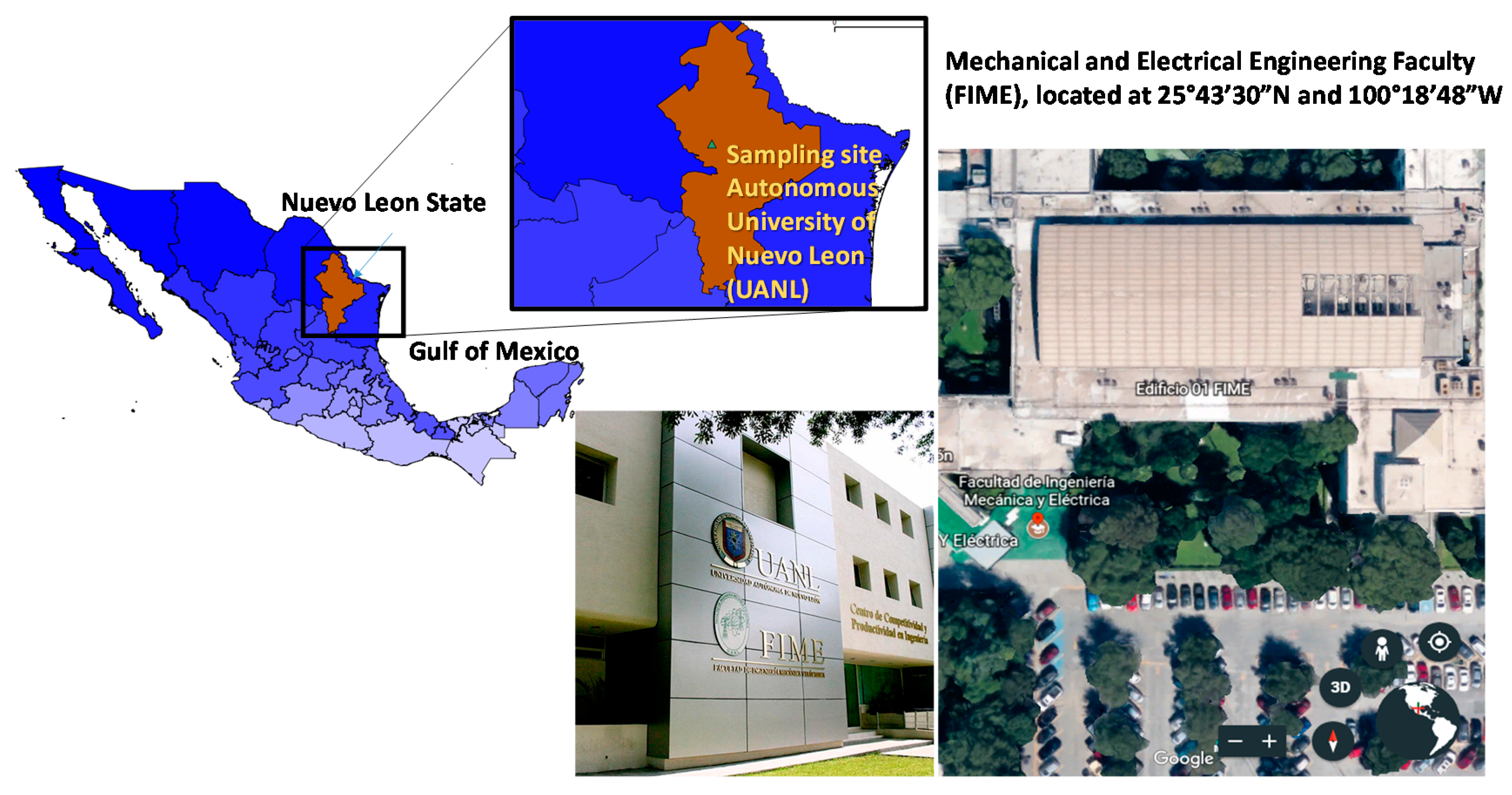
2.1. Sampling Site

This study focused on San Nicolas de los Garza, located in the northeast of MMA where industrial activities and vehicular traffic are common pollution sources. Air samples were collected on a rooftop (20 m above ground level) in the Mechanical and Electrical Engineering School building within the Autonomous University of Nuevo Leon (UANL) facilities (25°43′30″N; 100°18′48″W) (Figure 1). The sampling site is urban, located within an industrial, residential, and commercial area containing avenues with abundant vehicular traffic.

2.2. Statistical Analysis

The Friedman test was used to determine the difference of mean concentrations for benzene and carbonyls among differing sampling seasons and times of day. The Friedman test is a nonparametric test that can be used with block designs, and the underlying assumptions are not as restrictive as an ANOVA procedure. The technique is based on the ranks of the observations within each block (sampling season and diurnal sampling periods). The assumptions pertaining to this study are: (1) The results within one block do not influence the results within the other blocks; and (2) within each block, the observations may be ranked according to some criteria of interest. The hypotheses to be tested are: H0 “the samples come from the same population, that is, there are no significant differences between seasons or between time-of-day sampling periods”, and H1 “the samples did not come from the same population, that is, there are significant differences between seasons or between time-of-day sampling periods”. This analysis was applied to concentration dataset for benzene and carbonyls using XLSTAT statistical software (2016.5 version, New York, NY, USA) [18].

2.3. Measurement of VOCs (Carbonyls and Benzene), Meteorological Parameters, and Criteria Air Pollutants

2.3.1. Sampling and Analysis of Benzene

Benzene was measured in ambient air of the study site. 165 samples were collected from 8 August 2011 to 19 January 2012. Air samples were collected within glass tubes containing 226-01 Anasorb CSC (SKC) using a Universal XR pump model PCXR4 (SKC) at a flow rate of 200 mL min−1 (Method INSHT MTA/MA030/A92; INSHT 1992). 1.5 hour samples were collected during morning (9:00 to 10:30 a.m.), midday (noon to 1:30 p.m.) and afternoon (3:00–4:30 p.m.). After sampling, the adsorption tubes were labeled and capped tightly with PTFE caps and refrigerated until the chemical analysis (samples must be analyzed in a period no greater than 21 days after collection). Samples were analyzed at the Environmental Sciences Laboratory in the Autonomous University of Carmen City (UNACAR).
Collected samples were extracted with 1 mL of CS2 and then analyzed using a gas chromatograph (TRACE GC Ultra Thermo Fisher Scientific Technologies, Inc.; Waltham, MA, USA) and a flame ionization detector (Thermo Fisher Scientific Technologies, Inc.; Waltham, MA, USA) according to the MTA/MA030/A92 Method (INSHT 1992). The analytical column used was a capillary column (57 m, 0.32 mm i.d., 0.25 µm film thickness). The oven temperature program used in the gas chromatography analysis was the following: 40 °C for 4 min, with subsequent temperature increase at a rate of 5 °C/min to 100 °C and maintained for 10 min. Ultra-pure hydrogen and extra-dried air were used in the flame ionization detector (at constant flow: 35 mL min−1 and 350 mL min−1, respectively) and ultra-pure nitrogen (99.999%) was used as carrier gas at a flow rate of 1 mL min−1. The analytical method evaluation (QA/QC) was performed according to Cerón et al. [19]. Calibration with seven points was performed (from 0.10 to 100.00 µg/mL) using an analytical grade reagent of benzene (99.98% from Sigma Aldrich, St Louis, MO, USA). The method detection limit (MDL) for benzene was determined by multiplying the standard deviation obtained from seven replicate measurements of the first calibration level (0.10 µg/mL) by 1.943 (Student-t distribution value for n − 1 = 7 with a confidence of 95%). The MDL was 0.05 µg/mL and the relative standard deviation (RSD) was 8.04%. This value for the MDL is acceptable because the coefficient variation was less than 10%. Method accuracy was estimated through the analysis of seven replicates of benzene solution in the range of 0.10 to 100.00 µg/mL, obtaining an average of 1.03, a RSD of 3.20%, and average error of 2.50% and a linearity with R2 of 0.9998. The acceptance criterion for accuracy was achieved since the coefficient of variation was less than 10%. We can, therefore, establish that the analytical method is accurate and exact in the assessed range of concentration.
Although the analytical method may be used to determine other BTEX compounds, it was decided to consider only benzene because it is the most abundant compound and it has the greatest implications for public health.

2.3.2. Sampling and Analysis of Carbonyls

Formaldehyde and acetaldehyde measurements in ambient air were made from 8 August 2011 to 19 January 2012. Samples were collected at 1.5 h intervals: 9:00–10:30 a.m., noon—1:30 p.m. and 3:00–4:30 p.m. A total of 165 samples were collected. Ambient air was passed through Sep-Pack DNPH-Silica cartridges at a rate of 1800 mL min−1 [20]. The downstream end of the cartridge was connected to a calibrated flow meter. An ozone scrubber was placed upstream of the cartridge to avoid degradation of hydrazone derivatives. Each cartridge was sealed with Teflon® caps immediately after sampling, wrapped in aluminum foil and refrigerated. Refrigeration period prior to analysis should not exceed two weeks. A volume of 162 L was obtained during the sampling. Cartridge collection efficiency was determined by connecting two cartridges in series; values >95% for both carbonyls were obtained. The sample breakthrough of the cartridges is 500 ppbv (considering the combined concentrations of both carbonyls) when a volume of 162 L of air is sampled. Sampling and analytical precision was determined from four sampling devices co-located and simultaneously operated on six occasions; the relative standard deviations (RSD) ranged from 0.3% to 12.1%. Cartridge laboratory blanks and cartridge field controls were analyzed to determine background levels of DNPH derivatives. Carbonyl levels in cartridge field controls were similar to those of the cartridge laboratory blanks. Ambient carbonyl concentrations were corrected for cartridge field blanks. The formed 2,4-dinitrophenylhydrazones were eluted with 5 mL of acetonitrile and 20 μL this solution were analyzed by high performance liquid chromatography (HPLC) with an Agilent 1100 instrument coupled to a UV detector operated at 360 nm, using water-acetonitrile as a mobile phase in a pump gradient program proposed by Method TO-11 A [20], flowing at 1 mL min−1 and using a Zorbax ODS column (250 mm × 2.6 μm DI). Analytical detection limits for formaldehyde and acetaldehyde derivatives were 0.09 and 0.25 μg m−3, respectively, for a sampling volume of 162 L [21].

2.4. Measurements of Criteria Air Pollutants and Meteorological Parameters

Wind speed and direction, relative humidity, temperature, and solar radiation were also monitored from 8 August 2011 to 19 January 2012. A Davis Vantage Pro II portable meteorological station was used to measure the meteorological parameters. Wind roses were constructed using the software WRPLOT [22] for each day during the studied period. 24 h air mass back trajectories were calculated using the NOAA (National Oceanic Administration Agency, Silver Spring, MD, USA) HYSPLIT model in order to infer the probable origin of the air masses [23]. O3, NO, NO2, NOx, CO, and SO2 were measured using automatic analyzers (chemical luminescence, UV photometry, and UV fluorescence) (details about the specific instruments can be found within the Table S1 in Supplementary Material). The criteria air pollutant data were obtained from the Integrated Air Quality Monitoring System of the MMA (Northeast Station of the Atmospheric Monitoring System (SIMA) ), located in San Nicolas de los Garza, N.L. at 25° 44′ 42″ N and 100° 15′ 17″ W at 500 m a.s.l., 5.2 km from the sampling site.

2.5. Principal Component Analysis

Pearson correlations coefficients were determined for all data blocks. Factor analysis (principal component analysis) was applied to assess the relationships between carbonyls, benzene, and criteria air pollutant concentrations and meteorological parameters This method is a well-documented analysis tool for classifying, modelling and interpreting environmental monitoring data [24,25]. Interpretation of PCA results is usually carried out by visualization of the components scores and loadings. The software package used was XLSTAT version 2016.5 [18].

2.6. Health Risk Evaluation

Formaldehyde, acetaldehyde, and benzene have been classified by US Environmental Protection Agency [26] as carcinogenic compounds within groups B1, B2, and A, respectively, based on limited evidence of carcinogenicity in humans and sufficient evidence of carcinogenicity in animals [26,27]. Benzene has been classified as potentially carcinogenic (type I) according to the International Agency for Research on Cancer [28] due to its toxic effects in the central nervous system and in fetuses [29]. The US Environmental Protection Agency have established quantitative risk assessments for the cancer and non-cancer risks of VOCs [5,26]. To estimate these health risks we used the methodology described by Zhang and collaborators [30], considering only inhalation exposure. Daily exposure (E), the hazard quotient for non-hazard risk (HQ), and integrated lifetime cancer risks (ILTCR) were calculated using the following equations:
E = (C × IRa × DA) / BW
where E is the daily exposure expressed in mg/kg per day of an individual by inhalation, C (mg m−3) is the concentration of the air pollutant, IRa is the inhalation rate for adults (0.83 m3 h−1) [31], DA is the exposure duration of an adult (24 h/day), and BW is the body weight of an adult (65 kg) [26]. The integrated lifetime risk (ILTCR) is then calculated as follows:
ILTCR = E × SF
where SF is the slope factor (kg day/mg) of inhalation unit risk for toxics when the exposure-carcinogenic effect is considered as linear. We used SF values in Table 1, provided by the US EPA [32,33]. The non-cancer risk (HQ quotient) is calculated by dividing the yearly average daily-received concentration (CY) by the inhalation reference concentrations of the specific air pollutant (RfC values shown in Table 1)
HQ = CY / RfC
In addition, a hazardous index (HI) was estimated in order to obtain a measure of the overall potential for non-carcinogenic effects posed by more than one chemical. Using the total hazard quotient (∑HQ) for all the individual chemicals [29], a HQ > 1 indicates that long-term exposure may result in adverse health effects:
HI = ∑HQ

3. Results and Discussion

3.1. Diurnal and Seasonal Variations

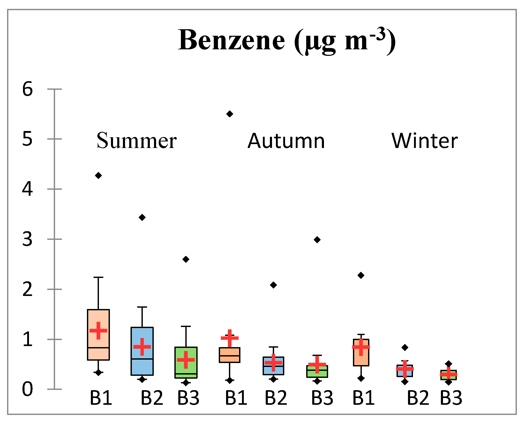
3.1.1. Results for Benzene

Diurnal and seasonal variation and parametric statistics for measured benzene are shown in Figure 2. The mean benzene concentration over the whole period was 0.65 μg m−3. Benzene exhibited a clear seasonal trend, with the highest concentrations during summer (0.8739 μg m−3), decreasing during autumn (0.6860 μg m−3), and reaching minimum values during winter (0.5186 μg m−3). The higher concentrations of benzene during summer may be explained by the potential contribution of fuel and solvent evaporation, which increases in response to the higher temperatures normally observed during this season in the study area. Mean summer benzene concentrations were significantly different than those of autumn and winter, however differences between mean autumn and winter concentrations were not significant (statistical significance corresponds to the 95% level as determined by the Friedman test—see the Table S2 in Supplementary Material). All benzene measurements exhibited a diurnal pattern with the highest concentrations occurring during the morning sampling period (B1), decreasing during midday (B2), and reaching a minimum during the afternoon sampling period (B3). During summer, benzene mean concentrations showed significant differences among the different diurnal sampling periods. During autumn and winter, mean concentrations during midday and afternoon were not significant. The elevated morning concentrations can be attributed to vehicular emissions during rush hour and also to the presence of thermal inversions. Pollutant concentrations are sensitive to the daily evolution of the boundary layer. Following the onset of solar radiation at sunrise, surface temperature and wind speed typically increase as the boundary layer height increases, mixing momentum from aloft and diluting contaminants. Continuing through midday, the deepening boundary layer (particularly during summer) provides a larger volume for the dilution of air pollutants, increasing dispersion and decreasing concentrations. In addition, the higher intensity of solar radiation during afternoon favors the photodecomposition of some air pollutants. At night, nocturnal cooling reduces surface temperature and mixing from aloft, often forming thermal inversions. Inversions, with their increased atmospheric stability and decreased dispersion potential, decrease the depth of the mixed layer and cause pollutants to become more concentrated.
The lower benzene concentrations found during midday (B2) and afternoon (B3) can be attributed to the faster removal of volatile organic compounds by reactions with hydroxyl (•OH) and nitrate (NO3) radicals due to enhanced solar radiation and temperature. Additionally, around noon, the increasing surface air temperature removes the thermal inversion and increases the mixed layer depth to its afternoon maximum. Menchaca-Torre et al. [42] observed the same behavior in afternoon benzene concentrations measured during 2011 and 2012 in a nearby location in Monterrey, including accelerated secondary pollutant production from photochemical reactions, decreasing VOC levels especially between 2:00 and 6:00 p.m.

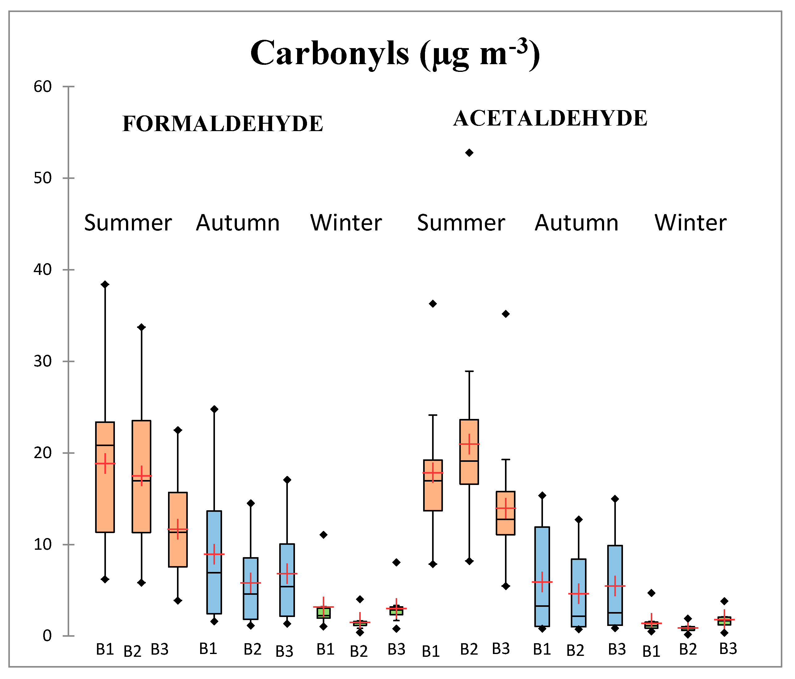
3.1.2. Results for C1-C2 Carbonyls

Parametric statistics, seasonal, and diurnal variation for formaldehyde and acetaldehyde concentrations are shown in Figure 3. Over the entire sampling period, formaldehyde was more abundant than acetaldehyde with concentrations of 9.06 μg m−3 and 8.06 μg m−3, respectively. Ambient carbonyls levels are influenced by various factors, including photochemical production and decomposition, combustion, and vehicular sources, and meteorological conditions (temperature, solar radiation, rainfall intensity, and wind speed). Formaldehyde showed a clear diurnal pattern with the highest mean concentrations during the morning sampling period (10.33 μg m−3 over in all climatic seasons). This behavior is in agreement with that reported by Menchaca-Torre et al. [43] and Facundo-Torres et al. [44] who found higher levels of formaldehyde during the morning in a location near the Metropolitan Area of Monterey. This can be explained by vehicular emissions, since the morning (B1) sampling period coincides with rush hour. During summer formaldehyde showed a different diurnal pattern (B1 > B2 > B3) as compared to autumn and winter seasons (B1 > B3 > B2). The Friedman test (see the Table S3 in Supplementary Material) revealed that there were significant differences in mean formaldehyde concentrations among different diurnal sampling periods, however, a bilateral test (Nemenyi procedure) by multiple comparisons in pairs showed that mean formaldehyde differences between the B1 and B2 sampling periods (morning and midday) during summer and between B1 and B3 (morning and afternoon) during autumn and winter were not significant. During summer mornings, in addition to the anthropogenic source contributions related to vehicular traffic, the conditions of sunlight and radiation were high (See Table 3), initiating photochemical activity from early hours. On the other hand, anthropogenic activity was the dominant source of formaldehyde during autumn and winter seasons.
Acetaldehyde concentrations also exhibited a diurnal pattern, but except for autumn this variability was different than that of formaldehyde. During summer higher concentrations occurred during midday sampling period (B2: 20.99 μg m−3), whereas during autumn and winter concentrations of this carbonyl were higher mean during the morning (B1: 5.93 μg m−3) and afternoon (B3: 1.82 μg m−3) sampling periods. According to the Friedman test results (see the Table S4 in Supplementary Material), differences of mean acetaldehyde levels among the different diurnal sampling periods were significant. However, as was the case for formaldehyde, the bi-lateral test by multiple comparison failed to show significant differences in acetaldehyde concentrations between B1 and B2 during summer, and between B1 and B3 during both autumn and winter.
During summer we found differences in diurnal behavior: formaldehyde was more concentrated in the morning, while acetaldehyde levels were higher during midday. This can be explained by the higher photolysis rate of formaldehyde, which increases its midday photodegradation relative to that of acetaldehyde. In addition, the longer lifetime of acetaldehyde favors accumulation and secondary formation through the reaction of other organic compounds.
On the other hand, the higher formaldehyde concentrations during mornings (summer) may be attributed to a combination of photochemical formation, since photo-oxidation of hydrocarbons in summer begins much earlier than in autumn and winter, and also to anthropogenic sources related to vehicular traffic (the morning sampling period coincides with the rush hour). The lower formaldehyde concentrations during midday (summer) can be explained due to photolysis loss. According to De Andrade et al. [45] the lifetime of formaldehyde is about 6.3 h in the summer and 8.1 h in the winter, due to photolysis, while the lifetime of acetaldehyde is about 3.3 days in the summer and five days in the winter. This can explain the different seasonal behavior of both carbonyls, and may also contribute to the decrease in formaldehyde concentrations during the day. Acetaldehyde levels increase and remain nearly constant because of the low reactivity of this compound, favoring accumulation, and secondary formation through the reaction of other organic compounds.
The two carbonyls exhibited different diurnal patterns during winter: formaldehyde levels were higher during morning, whereas acetaldehyde levels were higher during the afternoon. We can assume that during winter the carbonyls originate from different sources since they correlate neither with CO, nor between themselves. In addition, meteorological analysis showed that formaldehyde had its highest levels of concentration when the winds blew from the west (General Escobedo municipality) while acetaldehyde concentrations were highest when the air masses came from the north (Apodaca municipality).
During autumn both carbonyls behaved similarly throughout the day. Meteorological conditions during this season were relatively stable (lower wind speed values) compared with other seasons, and had less impact on the carbonyl concentrations. From the Pearson correlation analysis it was found that both carbonyls showed good correlation between each other and also have significant correlation with CO and solar radiation, indicating that they had sources in common.
On the other hand, both carbonyls had a marked seasonal trend, showing significant seasonal differences in accordance with the discriminant analysis (Friedman test, p-value < 0.0001) (see the Supplementary Material). The seasonal variation for both carbonyls was the following: summer (formaldehyde: 16.02 μg m−3, acetaldehyde: 17.60 μg m−3) > autumn (formaldehyde: 7.2 μg m−3, acetaldehyde: 5.35 μg m−3 > winter (formaldehyde: 2.56 μg m−3, acetaldehyde: 1.37 μg m−3). Carbonyls mass ratios for summer/winter and autumn/winter were 5.11 and 3.04, respectively, for formaldehyde; and 10.23 and 4.24, respectively, for acetaldehyde. These results suggest that carbonyls measured at the study site were influenced by mixed sources: secondary (photochemical activity) and primary sources (vehicular emissions), and meteorological conditions.
Higher levels of both carbonyls during summer and daytime (morning and midday) suggest that local photo-oxidation of hydrocarbons may be an important source of carbonyls at the study site. This is expected since temperature and sunlight intensity are higher during summer. It is well known that the behavior of air pollutants depends on many factors including development, urbanization, regulations, topography, climate, etc., and thus the spatial and temporal variation of pollutants and their sources varies from one location to another. However, it is interesting to compare the results found in this study with other cities around the world with an equal or greater degree of urbanization and development. We compared our results with those reported in other cities with similar population, with lower population like the Tri-City located in North Poland (Golansk, Gdynia, and Sopot), and with higher population like Nueva Delhi and Jinan. Table 2 shows a comparison of the average concentrations reported in this study with similar analyses reported for other locations around the world. Benzene concentrations in the three monitoring campaigns were similar to those obtained in North Poland by Marć et al. [46] and in Alicante, Spain by Galindo et al. [47], but lower than those reported by Liu et al. [48] in Jinan, China, and by Singh et al. [29] in Delhi, India. Alicante, Spain has similar population, population density and sources as compared to our study site (Table 2). Both North Poland cities have populations seven times less than the study site. All of these areas are classified as medium size cities. Jinan (China), Delhi (India) and Monterrey (Mexico) have larger population, surface area, and population density than the study site (excepting Monterrey, which has a lower population density than San Nicolás de los Garza), so it is expected that COV emissions will be higher in these megacities.
The formaldehyde and acetaldehyde concentrations in the present study were lower than those reported in downtown Monterrey, Nuevo Leon, Mexico by Menchaca-Torre et al. [42] and similar to those reported in Chendu (China) [49], but higher than those reported in Longmen Southern China during 2012–2013 by Guo et al. [50].
Monterrey and Chengdu have twice and 28 times the size of population than the study city (San Nicolás de los Garza), therefore, it is expected that the emissions of VOCs are higher in these cities, in comparison to the present study site. Menchaca-Torre et al. [42] reported a mean value for benzene of 1.5 µg/m3 for Obispado, which is located in the center of Monterrey near San Nicolas de los Garza). This is more than twice the value found in this study. In a second study [42] at this same site these authors reported formaldehyde and acetaldehyde values slightly higher than those reported in this study. The higher benzene concentrations reported at the Obispado site [42] are likely due to the Obispado site’s location not only within an industrial zone, but also 42 km from a Mexican Petroleum Company (PEMEX) refinery (Cadereyta, Nuevo Leon). Despite reporting higher mean concentrations, the diurnal variation in benzene reported by Menchaca et al. [42] was similar to that found in this study: VOCs exhibited a higher concentration in the 6:00–10:00 a.m. time interval, and decreased during the subsequent two sampling intervals. We found higher levels of benzene in other sampling carried out in the center of Monterrey during autumn 2013 [51]. During that study, transport of air masses from the ESE occurred, from the municipalities of Apodaca and Guadalupe, where important industries, high traffic volume, many oil and gas service stations, and the largest airport in this region are found.

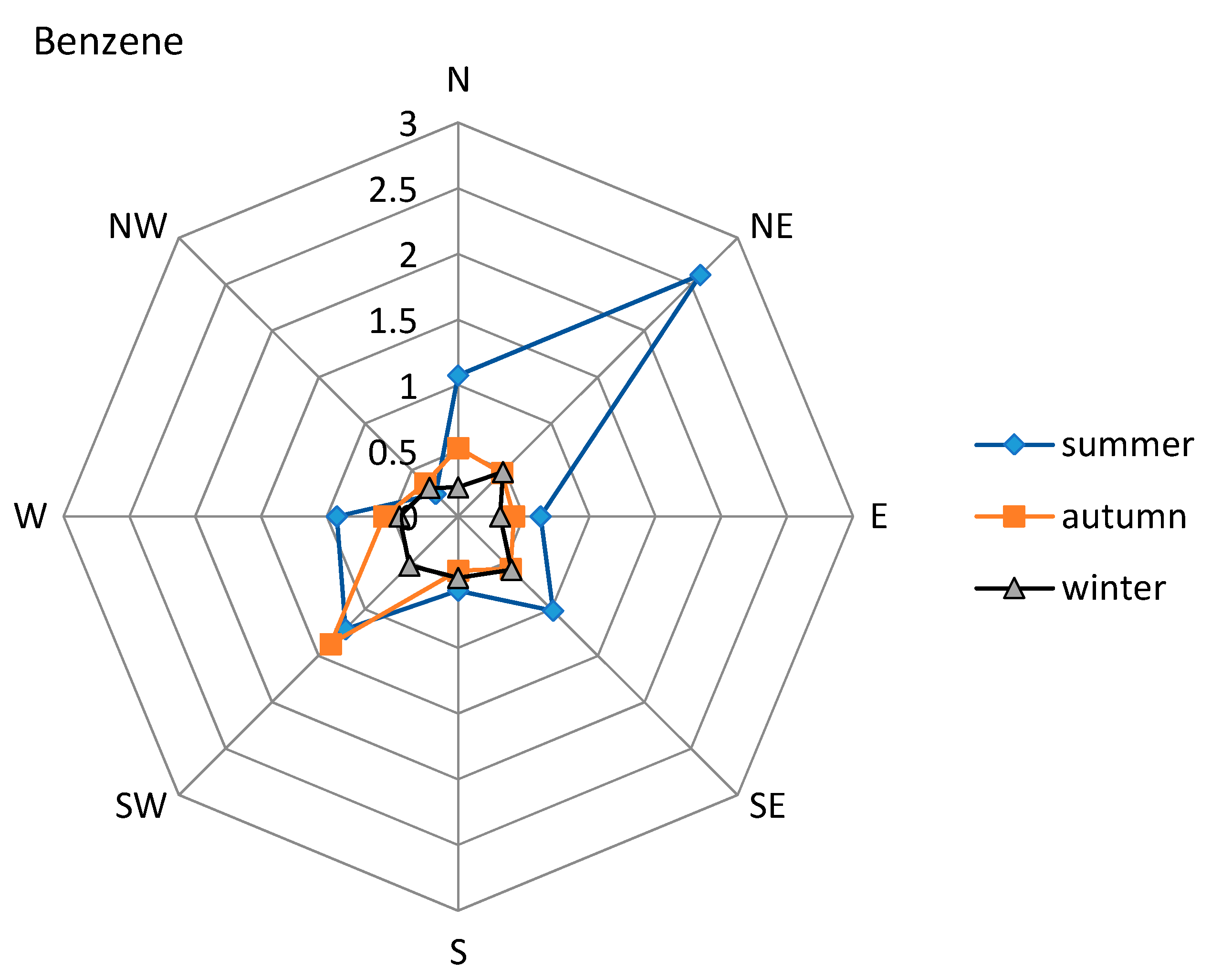
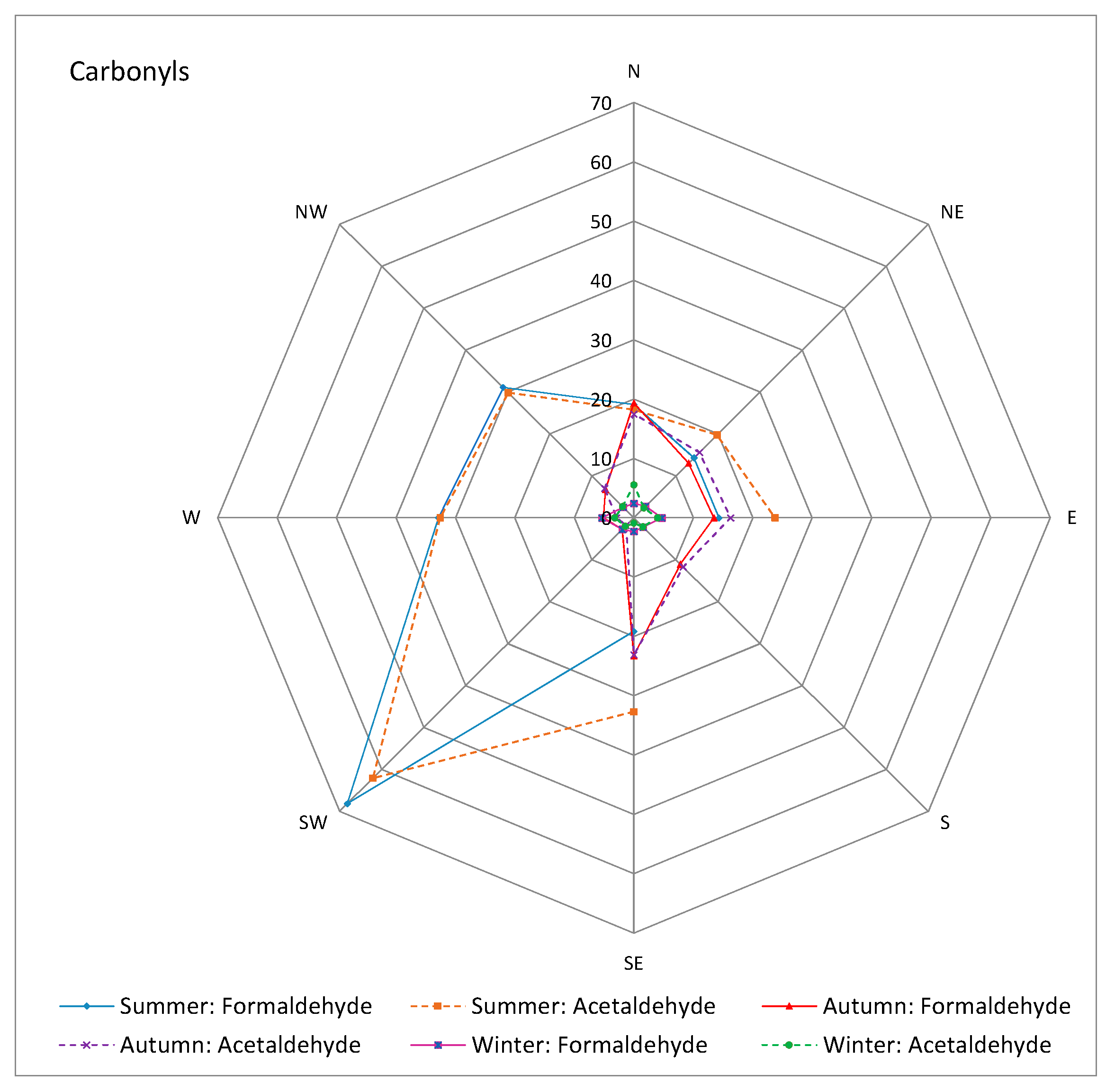
3.2. Meteorological Influence

Variations in VOCs with respect to wind direction have been studied in areas with industrial activity [43,52,53]. Meteorological conditions and criteria air pollutant concentrations (CO, NO, NO2, NOx, O3, and SO2) observed during the sampling campaigns are presented in Table 3. Temperature, solar radiation and wind speed were highest during the midday sampling period (B2), whereas relative humidity (RH) was highest during the morning sampling period (B1) for all seasonal campaigns. Wind direction changed during the morning and afternoon sampling periods, while during the midday sampling the wind direction was always NNE. During summer, autumn, and winter, average temperatures were 30.7 °C, 23.7 °C, and 15.5 °C, respectively. The average wind speed during summer, autumn, and winter was of 7.8 km h−1, 8 km h−1, and 7 km h−1, respectively. The average wind direction was predominantly NNE during summer, from ENE during autumn, and from ENE during winter. Pollutant dispersion characteristics of the region are strongly influenced by these local meteorological variables, and also by surrounding mountains which form a natural physical barrier to wind circulation. In addition, variations in atmospheric stability control the extent to which ground-level pollutants are mixed and diluted. Mixing is greatest during the afternoon, particularly during summer, in response to convection associated with high surface temperatures. Mixing is limited during the morning (B1) period, particularly during winter, when temperature inversions associated with nocturnal cooling commonly occur. CO and O3 showed similar seasonal behavior, with higher concentrations during summer. CO registered higher concentrations during the morning sampling period (B1) during autumn and winter, whereas O3 exhibited higher concentrations during the midday and afternoon sampling periods. NO showed higher concentrations during winter and the morning sampling period (B1). NO2 and NOx had higher levels of concentration during summer afternoon period. SO2 had higher concentration values during autumn and winter, and during the midday and afternoon sampling periods.
In this region, two scenarios could be observed, one for ozone and CO with peaks of concentration in summer period (when higher temperatures and solar radiation intensities are common, favor photochemical activity and tropospheric ozone production); and another scenario for the rest of air criteria pollutants (PM10, NOx, NO2, NO, SO2), which showed higher concentrations during autumn and winter periods, when specific atmospheric conditions are present (a lower boundary layer height, lower solar radiation intensities, higher atmospheric stability, mesoscale atmospheric systems, among which highlight the high pressure systems are prevalent in the cold season). It is important to note that the orographic and climatological conditions of this area favor the development of thermal inversions during early mornings and night, and during autumn and winter periods. This area has a complex orography that include a mountain system constituted by Sierra Madre Oriental, Loma Larga Hill, Las Mitras Hill, Huasteca Hill, and La Silla Hill, which affect ventilation conditions that may cause a mountain-valley effect, increasing air pollutants concentrations when winds remain below 2 km/h on the Beaufort scale.
Figure 4 and Figure 5 illustrate the variation in benzene and carbonyl concentrations with wind direction during summer, autumn, and winter. During summer benzene (Figure 4) showed higher concentrations when winds blew from the NE. During autumn, benzene concentrations were higher with SW winds. During winter sampling, benzene showed higher concentrations with winds from the SE. Formaldehyde and acetaldehyde (Figure 5) showed higher concentrations with SW and S winds during summer and autumn, respectively. During winter, on the other hand, formaldehyde and acetaldehyde showed higher concentrations when winds blew from W and N, respectively (Figure 5) (See also the Figure S1 in Supplementary Material). The municipality of General Escobedo is located to the NE of the sampling site, where the most important industrial area named “Escobedo Industrial Park” is located. Some important avenues with high vehicular traffic are located in this area: Sendero Norte Avenue, Universidad Avenue and the freeway to Nuevo Laredo. The municipality of Apodaca is located at N and NE of the sampling site. Established important companies and industries that produce lubricants, industrial additives, fertilizers, and steel products are located in this area, along with the Apodaca-Dr. Gonzalez road and the “Mariano Escobedo” international airport. The municipality of Monterrey and two important avenues (Morones Prieto and Ruiz Cortinez) are located S and SW of the sampling site, whereas the municipalities of Guadalupe, Juarez, and Cadereyta, where an oil refinery is located, are located to the SE. These industrial and vehicular sources associated with the main avenues and roads are possible contributors to the VOC concentrations sampled at this site during the sampling period.

3.3. Formaldehyde/Acetaldehyde Ratios

A formaldehyde/acetaldehyde ratio is commonly used to compare the results of carbonyl measurement studies at different locations [13,54]. In rural environments, values for this ratio between three and 10 have been reported [55,56]. The relatively high values for this ratio may reflect the local participation of natural reactive hydrocarbons whose oxidation yields more formaldehyde than acetaldehyde [57] or the influence of other important sources of formaldehyde, such as wood combustion [58]. In urban sites, several authors have reported values between 0.22 and 2.6 for this ratio [59,60]. In the present study, values for this ratio ranged from 0.25 to 6.15 during the sampling period (Table 4). Mean values were 0.96, 1.72, and 2.26 for summer, autumn, and winter, respectively. These values indicate that the production of C1-C2 carbonyls at the sampling site were strongly influenced by the local participation of anthropogenic hydrocarbons. The formaldehyde/acetaldehyde ratio usually varies from one to two for urban areas (large cities) to about 10 for forested rural areas. The high formaldehyde/acetaldehyde ratios may reflect the local participation of natural reactive hydrocarbons, such as isoprene, whose oxidation can yield more formaldehyde than acetaldehyde. Isoprene is a major reactive hydrocarbon that can yield a formaldehyde/acetaldehyde ratio of 10, and is mainly a biogenic emission. Values for this ratio lower than one may be found in sites such as Brazil, where oxygenated fuels are commonly used and where acetaldehyde emissions are higher than formaldehyde emissions. In San Nicolas de los Garza, gasoline is the most common fuel and vehicular emissions are the dominant source of VOCs. For this reason and according to the values reported in this study, the local participation of anthropogenic hydrocarbons appears to be important in the production of carbonyls, mainly vehicular emissions. Although caution is needed when comparing the levels of carbonyls among different locations (given differences in sources, fuel types, topography, climate, regulatory policies, among other factors), this reason constitutes a useful tool to understand the possible sources of carbonyls in a given area.
The formaldehyde/acetaldehyde ratios for this study agreed with reported typical values for urban areas, being greater for winter and autumn and lower for summer. This behavior can be understood by considering that in the study area, vehicular emissions are the principal source of carbonyls during winter season, while both vehicular emissions and photochemical reactions are the dominant sources in summer. In addition, the daytime photolysis rate for formaldehyde is larger than that for acetaldehyde, especially around noon and during the summer when solar radiation and photochemical activity are intense. This behavior results in higher levels of acetaldehyde than those registered for formaldehyde (lower formaldehyde/acetaldehyde ratios). It is known that formaldehyde is more associated with gasoline engine emissions than acetaldehyde [61]. Acetaldehyde is associated with other sources beyond vehicular traffic emissions, including restaurant emissions, area sources, and stationary emissions [62]. Comparing our results for formaldehyde/acetaldehyde ratio with those reported for other large cities around the world, we found that Beijing, China (Pang and Mu) [63] and Monterrey, Mexico (Menchaca-Torre et al.) [43] showed similar formaldehyde/acetaldehyde ratios: 2.7–3.9 and 0.86–1.94, respectively. These values are characteristic of urban areas. These cities have similar climate and carbonyl sources (vehicular traffic and photochemical activity) as the present study city. In addition the seasonal variation of air temperature and solar radiation are similar to that found here, causing that photochemical activity to be important in the partition of primary and secondary pollutants in the atmosphere. The location of the present study site is similar to the sampling sites in Beijing [63] and Monterrey [43], being surrounded by main streets; thus, vehicular emissions are among the main anthropogenic carbonyls sources.

3.4. Pearson Correlation and Principal Component Analysis (PCA)

Table 5, Table 6 and Table 7 show the bivariate correlation analysis (Pearson coefficients tables) among benzene, formaldehyde, acetaldehyde, meteorological parameters, and criteria air pollutants during summer, autumn, and winter, respectively. CO showed significant positive correlations with NOx, NO, NO2 and benzene during the three climatic periods, and with acetaldehyde and formaldehyde during the autumn season. CO is considered a tracer of vehicular emissions since in the Metropolitan Area of Monterrey (MMA), 96.5% of the total emissions of this pollutant come from mobile sources [16]. Vehicular traffic influenced the air ambient concentrations for all of these compounds in the study site. This behavior was expected since MMA has a motorization index of 415 vehicles/1000 inhabitants and a vehicular fleet of 1.7 million [64]. Of these, 52% correspond to private vehicles, 40% to pick-up trucks, 3% to trucks, 3% to taxis, and 1% to public transport. In addition, the MMA (2005) reported that 47.2% of the total VOC emissions come from mobile sources.
During summer (Table 5), a negative moderate correlation between CO and acetaldehyde was observed, (−0.506) indicating that photolysis of acetaldehyde may contribute to the formation of CO, since acetaldehyde has three possible decomposition channels [65], but the quantum yield for the third channel (Equation (7)) is <0.01 at all wavelengths above 290 nm and hence can be ignored:
CH3CHO + hv -------→ CH3 + HCO
CH3CHO + hv -------→ CH4 + CO
CH3CHO + hv -------→ CH3CO + H
Although the photolysis rate of acetaldehyde is lower than that for formaldehyde, during summer sampling solar radiation showed a non-significant negative correlation with acetaldehyde concentrations (−0.224), indicating that acetaldehyde photodecomposition occurred during this period (not significantly, but it occurred). At the same time, CO showed a moderate positive correlation with solar radiation (0.449), indicating that a small fraction of the measured CO could be photochemically derived and that another major fraction was emitted from primary sources (vehicular emissions). In addition, higher CO concentrations were found during the summer period, which may indicate that, in addition to vehicular traffic emissions, photochemical activity may have contributed to CO levels during this period. Horowitz and Calvert [66] and Horowitz et al. [67] reported that the second channel (Equation (6)) is an important source of CO from acetaldehyde photolysis due to CH4 and CO formation, not only in Equation (6) (second channel), but through the various possible interactions of the free radicals created in Equation (5) with one another and with acetaldehyde.
CO, NOx, NO2, and benzene showed negative significant correlations with ozone during the three sampling seasons, indicating that these compounds acted as ozone precursors. This is an indicator that photochemical activity was important at the study site.
During summer, solar radiation had a negative moderate correlation with formaldehyde (−0.421), indicating that photolysis during this period was an important sink for formaldehyde (it has been reported that summer photolysis rates are usually 1–2 orders of magnitude faster than autumn and winter). Acetaldehyde also correlated negatively with solar radiation, but this correlation was not significant, since acetaldehyde removal by photolysis is slower than for formaldehyde.
During summer (Table 5) solar radiation had significant negative correlations with ozone and SO2, indicating that SO2 suffered photochemical reactions resulting in its oxidation by O3 and other oxidants commonly present in photochemical smog, i.e., HO•, HOO•, O, NO3, N2O5, ROO•, and RO•. During autumn solar radiation had positive significant correlations with formaldehyde, acetaldehyde, and temperature, indicating that photochemical activity was an important source of these pollutants during this period. Photo-oxidation of hydrocarbons by OH or by reaction of ozone with unsaturated hydrocarbons leads to carbonyl formation. In the atmosphere, carbonyls are removed by photolysis (this process is more significant during summer) but at the same time, carbonyls may be formed by photo-oxidation of hydrocarbons via OH. The competition between photochemical formation (reactions of hydrocarbons with O) and photochemical removal (by photolysis) may result in a net production or a net loss of aldehydes.
Both carbonyls had moderate positive and significant correlations between each other during autumn (Table 6) and summer (Table 5), indicating that they also originate from common sources.
During winter formaldehyde and acetaldehyde did not correlate, indicating that these compounds had different sources. This winter behavior is verified by the wind analysis, as higher concentrations for formaldehyde were registered when the winds blew from the west (General Escobedo municipality) while acetaldehyde showed higher concentrations when the air blew from the north (Apodaca municipality).
PCA results are shown in Table 8. Two factors were required to explain almost 70% of the data variability during summer season. Only significant factor loadings are shown for each variable. The PC1 factor contains pollutants associated with vehicular emissions mainly from light vehicles using gasoline as a fuel (CO, NO2, NOx, formaldehyde, acetaldehyde, and benzene) and compounds related to photochemical activity (NO, O3, and SR). The separate PC2 factor pertains to solar radiation and SO2, a pollutant related to emissions from diesel vehicles and industrial sources. The PCA results are supported by the National Inventory of Emissions Results (SEMARNAT-INE, 2005). Total VOC emissions from vehicular sources in the Metropolitan Area of Monterrey (where San Nicolas de los Garza is located) are apportioned as follows: light vehicles using gasoline contribute 58%, light trucks using gasoline contribute 32%, heavy-duty vehicles using diesel contribute 5%, and the remaining 5% are due to other types of vehicles.
During autumn (Table 8), three principal components (PCs) were necessary to explain 75.18% of the total variance in the dataset: the PC1-factor (pollutants derived from light vehicular emissions) containing CO, NOx, NO, NO2, and benzene; the PC2-factor containing SO2 and relative humidity, indicating that this pollutant was removed from the air column by washout processes; the PC3-factor, which includes variables related to photochemical activity (T, O3, SR, formaldehyde, and acetaldehyde).
During winter, two factors (PCs) were required to explain almost 94% of the variability of data (Table 8): the PC1-factor (pollutants derived from light vehicular emissions) containing higher loads for CO, NOx, NO, NO2,, and benzene and the PC2-factor containing only SO2, with a separate impact, which can be an indicator that this compound has different sources in the study site (98.3% of this compound in San Nicolas de los Garza is emitted from industrial sources, and only 1.5% of the total emissions come from mobile sources using diesel as fuel).
These results suggest that benzene and carbonyls in the study site were influenced by mixed sources: secondary (photochemical activity) and primary sources (vehicular sources).

3.5. Health Risk

The estimated values for average daily exposure are shown in Table 9. Estimated values of ILTCR and HQ for formaldehyde, acetaldehyde, and benzene at the study site are listed in Table 10 and compared with results of other studies. Daily average exposures (mg/kg per day) are found to vary from 7.42 × 10⁻⁵ to 4.67 × 10⁻³ with greater exposure values for children. The individual non-cancer risk quotients (HQ) for each toxic air pollutant was <1, indicating that long-term exposure to these compounds still may not represent a health risk. However, if atmospheric formaldehyde concentrations are not controlled in San Nicolas de los Garza, it may cause adverse effects to health since its HQ value is close to unity. The cumulative non-cancer risk, measured as a hazardous index (HI) considering the hazard quotient for each air pollutant, resulted in a value of 1.83 which exceeds the threshold value (1.0) at the study site. The estimated cancer risks (ILTCR values) found in the present study for adults and children ranged from 3.05 × 10⁻⁶ to 6.11 × 10⁻⁵, which are higher than the 1 × 10⁻⁶ guideline established by the US EPA [26,68]. ILTCR values for both carbonyls exceeded the threshold value established by the World Health Organization (1 × 10⁻⁵) [5]. Comparing HQ and ILTCR values found in this study with those reported in other industrial cities around the world, we found that formaldehyde showed a higher ILTCR value than Kolkata and Bangkok, but lower than that reported for Beijing. Estimated values for risk cancer for acetaldehyde were higher than those reported for Beijing, Bangkok and Kolkata. The estimated ILTCR value for benzene in San Nicolas de los Garza was lower than that reported in Beijing and Kolkata. According to Sexton et al. [69], cancer risks can be classified into three broad groups: a) as definitive risk if ILTCR > 1.0 × 10⁻⁴; b) probable risk if 1 × 10⁻⁵ < ILTCR < 1 × 10⁻⁴; and c) possible risk if 1 × 10⁻⁶ < ILTCR < 1 × 10⁻⁵. Based on this classification, we conclude that the population in San Nicolas de los Garza is at possible risk of contracting cancer from inhalation exposure to these compounds.

4. Conclusions

All benzene measurements exhibited a diurnal pattern with the highest concentrations occurring during the morning sampling period. This behavior was to be expected as it coincides with the rush hour of vehicular traffic, as well as the formation of thermal inversions in the study area. The lower benzene concentrations found during midday and afternoon can be attributed to removal processes by photochemical reactions due to enhanced solar radiation and temperature. Benzene concentrations were largest during summer and decreased during winter. Formaldehyde was more abundant than acetaldehyde and showed a clear diurnal pattern with the highest mean concentrations during the morning sampling period. During summer, formaldehyde showed a different diurnal pattern (morning > midday > afternoon) as compared to autumn and winter seasons (morning > afternoon > midday). Acetaldehyde did not show a clear diurnal pattern: during summer higher concentrations occurred during the midday period, whereas during autumn and winter, the mean concentrations of this carbonyl were higher during the morning and afternoon periods. Both carbonyls showed differences in their diurnal behavior during summer, this can be explained due to differences in their photolysis rate (formaldehyde is photo-degraded faster than acetaldehyde) and atmospheric lifetimes (formaldehyde’s lifetime is much shorter than acetaldehyde’s).
Meteorological analysis revealed that sources to the NE and SW of the sampling site (avenues with high vehicular traffic, and commercial and industrial areas) are likely contributors to the measured benzene levels, and sources located to the SW and S of the study site could contribute to carbonyl levels.
Formaldehyde/acetaldehyde concentration ratios indicated that the production of C1-C2 carbonyls at the sampling site were strongly influenced by the local participation of anthropogenic hydrocarbons.
From the PCA results we could find that vehicular traffic influenced the air ambient concentrations for all measured compounds in the study site during the three sampling periods. Photochemical activity was important at the study site since CO, NOx, NO2, and benzene showed negative significant correlations with ozone during the three sampling seasons. NO, NOx, and NO2 had positive significant correlations between each other during all the study, suggesting that they originated from common sources. Both carbonyls had sources in common during autumn but different sources during summer and winter, due to they probably originated from sources other than vehicular traffic and photochemical activity, most likely from area sources, including evaporative emissions, painting, cooking processes, storage, and distribution stations of gasoline and petroleum liquefied gas, among others.
A health risk assessment showed that exposure to carbonyls and benzene exceeded the value of 1 × 10⁻⁶ for the integrated lifetime cancer risk. Individual values for the hazard quotient (HQ) for each air pollutant considered did not exceed unity; however, a synergic effect should be considered since the sum of HQ individual values was greater than 1.0. We conclude that the population of San Nicolas de los Garza has a probable risk of suffering cancer in its lifetime due to inhalation exposure to these compounds. It is, therefore, necessary to improve the environmental policies to control benzene and carbonyl levels in San Nicolas de los Garza. These strategies could include changes in policies related to transport systems, promoting the usage of alternative energy sources, and especially improved control of area source emissions.

Supplementary Materials

The following are available online at https://www.mdpi.com/2073-4433/8/10/196/s1.

Acknowledgments

We appreciate the support provided by The Atmospheric Monitoring System (SIMA) belonging to the Office of Urban Development and the Environment of the Nuevo Leon State (SIMA Monterrey).

Author Contributions

Julia Griselda Cerón Bretón and Rosa María Cerón Bretón designed the experiment, analyzed the data and carbonyls samples by HPLC-UV, and wrote the paper; María de la Luz Espinosa Fuentes, Jonathan D. W. Kahl, and Evangelina Ramírez Lara carried out the statistical and meteorological analysis; Reyna del Carmen Lara-Severino and Marcela Rangel Marrón conducted the fieldwork; and Martha Patricia Uc Chi carried out chemical analysis by GC-FID.

Conflicts of Interest

The authors declare no conflict of interest.

References

  1. National Research Council (NRC). Human Exposure to Airborne Pollutants: Advances and Opportunities; National Academy Press: Washington, DC, USA, 1991. [Google Scholar]
  2. Atkinson, R. Atmospheric chemistry of VOCs and NOX. Atmos. Environ. 2000, 34, 2063–2101. [Google Scholar] [CrossRef]
  3. Hoque, R.R.; Khillare, P.S.; Agarwal, T.; Shridhar, V.; Balachandran, S. Spatial and temporal variation of BTEX in the urban atmosphere of Delhi, India. Sci. Total Environ. 2008, 392, 30–40. [Google Scholar] [CrossRef] [PubMed]
  4. Báez, A.; Padilla, H.; Garcia, R.; Torres, M.C.; Rosas, I.; Belmont, R. Carbonyl levels in indoor and outdoor air in Mexico City and Xalapa, Mexico. Sci. Total Environ. 2003, 302, 211–226. [Google Scholar] [CrossRef]
  5. WHO Regional Publications. Air Quality Guidelines for Europe. Available online: http://www.euro.who.int/__data/assets/pdf_file/0005/74732/E71922.pdf (accessed on 16 August 2017).
  6. Civan, M.Y.; Elbir, T.; Seyfioglu, R.; Kuntasal, Ö.O.; Bayram, A.; Doğan, G.; Yurdakul, S.; Andiç, Ö.; Müezzinoğlu, A.; Sofuoglu, S.C.; et al. Spatial and temporal variations in atmospheric VOCs, NO2, SO2, and O3 concentrations at a heavily industrialized region in Western Turkey, and assessment of the carcinogenic risk levels of benzene. Atmos. Environ. 2015, 103, 102–113. [Google Scholar] [CrossRef]
  7. De Blas, M.; Navazo, M.; Alonso, L.; Durana, N.; Gomez, M.C.; Iza, J. Simultaneous indoor and outdoor on-line hourly monitoring of atmospheric volatile organic compounds in an urban building. The role of inside and outside sources. Sci. Total Environ. 2012, 426, 327–335. [Google Scholar] [CrossRef] [PubMed]
  8. Anderson, L.G.; Lanning, J.A.; Barrell, R.; Miyagishima, J.; Jones, R.H.; Wolfe, P. Sources and sinks of formaldehyde and acetaldehyde: An analysis of Denver’s ambient concentration data. Atmos. Environ. 1996, 30, 2113–2123. [Google Scholar] [CrossRef]
  9. Wang, X.M.; Sheng, G.Y.; Fu, J.M.; Chan, C.Y.; Lee, S.C.; Chan, L.Y.; Wang, Z.S. Urban roadside aromatic hydrocarbons in three cities of the Pearl River Delta, People’s Republic of China. Atmos. Environ. 2002, 36, 5141–5148. [Google Scholar] [CrossRef]
  10. Vega, E.; Mugica, V.; Carmona, R.; Valencia, E. Hydrocarbon source apportionment in Mexico City using the chemical mass balance receptor model. Atmos. Environ. 2000, 34, 4121–4129. [Google Scholar] [CrossRef]
  11. Mugica, V.; Watson, J.; Vega, E.; Reyes, E.; Ruiz, M.E.; Chow, J. Receptor Model source apportionment of nonmethane hydrocarbons in Mexico City. Sci. World J. 2002, 2, 844–860. [Google Scholar] [CrossRef] [PubMed]
  12. Arriaga-Colina, J.L.; West, J.J.; Sosa, G.; Escalona, S.S.; Ordúñez, R.M.; Cervantes, A.D.M. Measurements of VOCs in Mexico City (1992–2001) and evaluation of VOCs and CO in the emissions inventory. Atmos. Environ. 2004, 38, 2523–2533. [Google Scholar] [CrossRef]
  13. Cerón, R.M.; Cerón, J.G.; Muriel, M. Diurnal and seasonal trends in carbonyl levels in a semi-urban coastal site in the Gulf of Campeche, Mexico. Atmos. Environ. 2007, 41, 63–71. [Google Scholar] [CrossRef]
  14. Cerón, J.G.; Ramírez, E.; Cerón, R.M.; Carballo, C.; Aguilar, C.; López, U.; Ramírez, A.; Gracia, Y.; Naal, D.; Campero, A.; et al. Diurnal and seasonal variation of BTX in ambient air of one urban site in Carmen City, Campeche, Mexico. J. Environ. Prot. 2013, 4, 40–49. [Google Scholar] [CrossRef]
  15. National Institute of Statistics and Geography (INEGI). Statistical Yearbook. Nuevo Leon. Mexico. 2011. Available online: http://www.beta.inegi.org.mx/app/biblioteca/ficha.html?upc=702825202019 (accessed on 27 June 2017).
  16. Secretary of Environment and Natural Resources SEMARNAT. INE. Emissions Inventory of the North Frontier States of Mexico. 2005. Available online: http://www3.cec.org/islandora/es/item/2204a-inventario-de-emisiones-de-los-estados-de-la-frontera-norte-de-mexico-1999-summary-es.pdf (accessed on 5 June 2017).
  17. Ortínez, A.; Mateos, A. Evaluación Preliminar de las Condiciones Atmosféricas y Climatología Química en el Área Metropolitana de Monterrey. Available online: http://aire.nl.gob.mx/rep_pm2_5.html (accessed on 27 June 2017).
  18. Statistical Software and Data Analysis Add-on for Excel (XLSTAT), 2016.5 Version. Available online: https://www.xlstat.com/en/ (accessed on 27 March 2017).
  19. Cerón, J.G.; Cerón, R.M.; Vivas, F.; Barceló, C.; Espinosa, M.L.; Ramírez, E.; Rangel, M.; Montero, J.A.; Rodríguez, A.; Uc, M.P. Characterization and sources of Aromatic Hydrocarbons (BTEX) in the atmosphere of two urban sites located in Yucatan Peninsula in Mexico. Atmosphere 2017, 8, 107. [Google Scholar]
  20. United States Environmental Protection Agency (USEPA). Determination of Formaldehyde in Ambient Air Using Adsorbent Cartridge Followed by High Performance Liquid Chromatography (HPLC). Available online: https://www3.epa.gov/ttnamti1/files/ambient/airtox/to-11ar.pdf (accessed on 21 June 2017).
  21. Miller, J.C.; Miller, J.N. Estadística Para Química Analítica, 1st ed.; Addison-Wesley Iberoamericana: Wilmington, DE, USA, 1993; ISBN 0-201-60140-0. [Google Scholar]
  22. Lakes Environmental. WRPLOT View Version 7.0: Wind Rose Plots for Meteorological Data. 2011. Available online: http://www.weblakes.com/products/wrplot/index.html (accessed on 23 July 2017).
  23. Air Resources Laboratory (ARL). HYSPLIT: Hybrid Single-Particle Lagrangian Integrated Trajectory. Available online: http://www.ready.noaa.gov/READYcmet.php (accessed on 22 July 2017).
  24. Geng, F.; Cai, C.; Tie, X.; Yu, Q.; An, J.; Peng, L.; Zhou, G.; Xu, J. Analysis of VOC emissions using PCA/APCS receptor model at city Shanghai, China. J. Atmos. Chem. 2009, 62, 229–247. [Google Scholar] [CrossRef]
  25. Vukovich, F.M. Weekday/Weekend differences in OH reactivity with VOCs and CO in Baltimore, Maryland. J. Air Waste Manag. Assoc. 2000, 50, 1843–1851. [Google Scholar] [CrossRef] [PubMed]
  26. United States Environmental Protection Agency (USEPA). Guidelines for Carcinogen Risk Assessment. Risk Assessment Forum. Available online: https://ofmpub.epa.gov/eims/eimscomm.getfile?p_download_id=437005 (accessed on 28 July 2017).
  27. International Agency for Research on Cancer (IARC). Monographs on the Evaluation of Carcinogenic Risk to Humans. Available online: http://monographs.iarc.fr/ENG/Monographs/vol109/mono109.pdf (accessed on 23 July 2017).
  28. International Agency for Research on Cancer (IARC). Monographs on the Evaluation of Carcinogenic Risk to Humans, Formaldehyde, 2-Butoxyethanol and 1-tert-Butoxypropan-2-ol. Available online: http://monographs.iarc.fr/ENG/Monographs/vol88/mono88.pdf (accessed on 23 July 2017).
  29. Singh, D.; Kumar, A.; Singh, B.P.; Anandam, K.; Singh, M.; Mina, U.; Kumar, K.; Jain, V.K. Spatial and Temporal variability of VOCs and its source estimation during rush/non-rush hours in ambient air of Delhi, India. Air Qual. Atmos. Health 2016, 9, 483–493. [Google Scholar] [CrossRef]
  30. Zhang, Z.; Wang, X.; Zhang, Y.; Lü, S.; Huang, Z.; Huang, X.; Wang, Y. Ambient air benzene at background sites in China’s most developed coastal regions: Exposure levels, source implications and health risks. Sci. Total Environ. 2015, 511, 792–800. [Google Scholar] [CrossRef] [PubMed]
  31. United States Environmental Protection Agency (USEPA). Integrated Risk Information System (IRIS); US Environmental Protection Agency: Washington, DC, USA, 1998.
  32. United States Environmental Protection Agency (USEPA). Guidelines for Carcinogen Risk Assessment. In Risk Assessment Forum; U.S. Environmental Protection Agency: Washington, DC, USA, 2005. [Google Scholar]
  33. United States Environmental Protection Agency (USEPA). Risk Assessment Guidance for Superfund Volume I: Human Health Evaluation Manual Part F, Supplemental Guidance for Inhalation Risk Assessment: Final; Office of Superfund Remediation and Technology Innovation, Environmental Protection Agency: Washington, DC, USA, 2009.
  34. US Department of Health and Human Services (US DHHS). Public Health Service. In Toxicological Profile for Benzene; Agency for Toxic Substances and Disease Registry: Atlanta, GA, USA, 2007. Available online: https://www.atsdr.cdc.gov/toxprofiles/tp3.pdf (accessed on 12 July 2017).
  35. The Risk Assessment Information System (RAIS). RAIS Toxicity and Properties. Chemical Values for Acetaldehyde. Available online: https://rais.ornl.gov/cgi-bin/tools/TOX_search (accessed on 10 April 2017).
  36. The Risk Assessment Information System (RAIS). RAIS Toxicity and Properties. Chemical Values for Formaldehyde. Available online: https://rais.ornl.gov/cgi-bin/tools/TOX_search (accessed on 10 April 2017).
  37. United States Environmental Protection Agency (USEPA). Toxicological Review of Benzene (Noncancer Effects) (CAS No. 71–43–2). In Support of Summary Information on the Integrated Risk Information System (IRIS) EPA/635/R-02/001F; U.S. Environmental Protection Agency: Washington, DC, USA, 2002. Available online: https://cfpub.epa.gov/ncea/iris/iris_documents/documents/toxreviews/0276tr.pdf (accessed on 23 May 2017).
  38. United States Environmental Protection Agency (USEPA). Risk Assessment for Carcinogenic Effects. Available online: https://www.epa.gov/fera/risk-assessment-carcinogenic-effects (accessed on 16 May 2017).
  39. United States Environmental Protection Agency (USEPA). An SAB Report: Formaldehyde Risk Assessment Update—Review of the Office of Toxic Substance’s Draft Formaldehyde Risk Assessment Update by the Environmental Protection Agency. Available online: https://nepis.epa.gov/Exe/ZyNET.exe/9100CAMU.TXT?ZyActionD=ZyDocument&Client=EPA&Index=1991+Thru+1994&Docs=&Query=&Time=&EndTime=&SearchMethod=1&TocRestrict=n&Toc=&TocEntry=&QField=&QFieldYear=&QFieldMonth=&QFieldDay=&IntQFieldOp=0&ExtQFieldOp=0&XmlQuery=&File=D%3A%5Czyfiles%5CIndex%20Data%5C91thru94%5CTxt%5C00000023%5C9100CAMU.txt&User=ANONYMOUS&Password=anonymous&SortMethod=h%7C-&MaximumDocuments=1&FuzzyDegree=0&ImageQuality=r75g8/r75g8/x150y150g16/i425&Display=hpfr&DefSeekPage=x&SearchBack=ZyActionL&Back=ZyActionS&BackDesc=Results%20page&MaximumPages=1&ZyEntry=1&SeekPage=x&ZyPURL (accessed on 6 June 2017).
  40. International Agency for Research on Cancer (IARC). IARC Monographs on the Evaluation of the Carcinogenic Risk of Chemicals to Humans: Allyl Compounds, Aldehydes, Epoxides and Peroxides. Volume 36. World Health Organization, Lyon, 1985. Available online: https://monographs.iarc.fr/ENG/Monographs/vol1–42/mono36.pdf (accessed on 14 June 2017).
  41. United States Environmental Protection Agency (USEPA). Carcinogenic Effects of Benzene: An Update. EPA/600/P-97/001F April 1998; National Center for Environmental Assessment–Washington Office: Office of Research and Development U.S. Environmental Protection Agency: Washington, DC, USA, 1998. Available online: https://webcache.googleusercontent.com/search?q=cache:yrS9K6L5IQoJ:https://ofmpub.epa.gov/eims/eimscomm.getfile%3Fp_download_id%3D428659+&cd=2&hl=es-419&ct=clnk&gl=mx (accessed on 26 June 2017).
  42. Menchaca-Torre, H.L.; Mercado-Hernandez, R.; Mendoza-Dominguez, A. Diurnal and seasonal variation of volatile organic compounds in the atmosphere of Monterrey, Mexico. Atmos. Pollut. Res. 2015, 6, 1073–1081. [Google Scholar] [CrossRef]
  43. Menchaca-Torre, H.L.; Mercado-Hernández, R.; Rodríguez-Rodríguez, J.; Mendoza-Domínguez, A. Diurnal and seasonal variations of carbonyls and their effect on ozone concentrations in the atmosphere of Monterrey, Mexico. J. Air Waste Manag. Assoc. 2015, 65, 500–510. [Google Scholar] [CrossRef] [PubMed]
  44. Facundo-Torres, D.M.; Ramírez-Lara, E.; Cerón-Bretón, J.G.; Cerón-Bretón, R.M.; García-Vasquez, Y.; Miranda-Guardiola, R.; Rivera de la Rosa, J. Measurement of Carbonyls and its relation with Criteria Pollutants (O3, NO, NO2, NOx, CO and SO2) in an Urban site within the metropolitan area of Monterrey, in Nuevo León, México. Int. J. Energy Environ. 2012, 6, 524–531. [Google Scholar]
  45. De Andrade, J.B.; Andrade, M.V.; Pinheiro, H.L.C. Atmospheric Levels of Formaldehyde and Acetaldehyde and their Relationship with the Vehicular Fleet Composition in Salvador, Bahia, Brazil. J. Braz. Chem. Soc. 1998, 9, 219–223. [Google Scholar] [CrossRef]
  46. Marć, M.; Bielawska, M.; Simeonov, V.; Namieśnik, J.; Zabiegala, B. The effect of anthropogenic activity on BTEX, NO2, SO2 and CO concentrations in urban air of the spa city of Sopot and medium-industrialized city of Tczew located in North Poland. Environ. Res. 2016, 147, 513–524. [Google Scholar] [CrossRef] [PubMed]
  47. Galindo, N.; Varea, M.; Gil-Moltó, J.; Yubero, E. BTX in urban areas of eastern Spain: A focus on time variations and sources. Environ. Sci. Pollut. Res. 2016, 23, 18267–18276. [Google Scholar] [CrossRef] [PubMed]
  48. Liu, Z.; Li, N.; Wang, N. Characterization and Source identification of ambient VOCs in Jinan, China. Air Qual. Atmos. Health. 2016, 9, 285–291. [Google Scholar] [CrossRef]
  49. Ho, K.F.; Hang, H.S.S.; Huang, R.J.; Dai, W.T.; Cao, J.J.; Tian, L.; Deng, W.J. Spatiotemporal distribution of carbonyl compounds in China. Environ. Pollut. 2015, 197, 316–324. [Google Scholar] [CrossRef] [PubMed]
  50. Guo, S.; He, X.; Chen, M.; Tan, J.; Wang, Y. Photochemical production of atmospheric carbonyls in a rural area in Southern China. Arch. Environ. Contam. Toxicol. 2014, 66, 594–605. [Google Scholar] [CrossRef] [PubMed]
  51. Cerón-Bretón, J.G.; Cerón-Bretón, R.M.; Kahl, J.D.W.; Ramírez-Lara, E.; Guarnaccia, C.; Aguilar-Ucán, C.; Montalvo-Romero, C.; Anguebes-Franseschi, F.; López-Chuken, U. Diurnal and seasonal variation of BTEX in the air of Monterrey, Mexico: Preliminary study of sources and photochemical ozone pollution. Air Qual. Atmos. Health 2015, 8, 469–482. [Google Scholar] [CrossRef]
  52. Srivastava, A.; Joseph, A.E.; Devotta, S. Volatile organic compounds in ambient air of Mumbai-India. Atmos. Environ. 2006, 40, 892–903. [Google Scholar] [CrossRef]
  53. Badol, C.; Locoge, N.; Galloo, J.C. Using a source-receptor approach to characterise VOC behaviour in a French urban area influenced by industrial emissions: Part II: Source contribution assessment using the Chemical Mass Balance (CMB) model. Sci. Total Environ. 2008, 389, 429–440. [Google Scholar] [CrossRef] [PubMed]
  54. Grosjean, D.; Williams, E.L., II; Grosjean, E. Peroxyacyl nitrates at southern California mountain forest locations. Environ. Sci. Technol. 1993, 27, 110–121. [Google Scholar] [CrossRef]
  55. Shepson, P.B.; Hastie, D.R.; Schiff, H.I.; Polizzi, M.; Bottenheim, J.W.; Anlauf, K.; Mackay, G.I.; Karecki, D.R. Atmospheric concentrations and temporal variations of C1–C3 carbonyl compounds at two rural sites in central Ontario. Atmos. Environ. 1991, 25, 2001–2015. [Google Scholar] [CrossRef]
  56. Jacob, D.J.; Wofsy, S.C. Photochemistry of biogenic emissions over the Amazon forest. J. Geophys. Res. 1988, 93, 1477–1486. [Google Scholar] [CrossRef]
  57. Lloyd, A.C.; Atkinson, R.; Lurmann, F.W.; Nitta, B. Modelling potential ozone impacts from natural hydrocarbons-I. Development and testing of a chemical mechanism for the NOx-air photooxidations of isoprene and α-pinene under ambient conditions. Atmos. Environ. 1983, 17, 1931–1950. [Google Scholar] [CrossRef]
  58. Hellén, H.; Hakola, H.; Pirjola, L.; Laurila, T.; Pystynen, K.H. Ambient air concentrations, source profiles and source apportionment of 71 different C2-C10 volatile organic compounds in urban and residential areas of Finland. Environ. Sci. Technol. 2006, 40, 103–108. [Google Scholar] [CrossRef] [PubMed]
  59. Ho, K.F.; Lee, S.C.; Louie, P.K.K.; Zou, S.C. Seasonal variation of carbonyl compound concentrations in urban area of Hong Kong. Atmos. Environ. 2002, 36, 1259–1265. [Google Scholar] [CrossRef]
  60. Okada, Y.; Nakagoshi, A.; Tsurukawa, M.; Matsumura, C.; Eiho, J.; Nakano, T. Environmental risk assessment and concentration trend of atmospheric volatile organic compounds in Hyogo Prefecture, Japan. Environ. Sci. Pollut. Res. 2012, 19, 201–213. [Google Scholar] [CrossRef] [PubMed]
  61. Báez, A.P.; Padilla, H.; Cervantes, J.; Pereyra, D.; Torres, M.C.; Garcia, R.; Belmont, R. Preliminary study of the determination of ambient carbonyls in Xalapa City, Veracruz, Mexico. Atmos. Environ. 2001, 35, 1813–1819. [Google Scholar] [CrossRef]
  62. Alves, C.A.; Evtyugina, M.; Cerqueira, M.; Nunes, T.; Duarte, M.; Vicente, E. Volatile organic compounds emitted by the stacks of restaurants. Air Qual. Atmos. Health 2014, 8, 401–412. [Google Scholar] [CrossRef]
  63. Pang, X.; Mu, X. Seasonal and diurnal variations of carbonyl compounds in Beijing ambient air. Atmos. Environ. 2006, 40, 6313–6320. [Google Scholar] [CrossRef]
  64. National Institute of Statistics, Geography and Informatics (INEGI). Environmental Statistics for the Metropolitan Area of Monterrey in 2001. Available online: www.inegi.gob.mx (accessed on 17 June 2017).
  65. Finnlayson-Pitss, B.J.; Pitts, J.N. Chemistry of the Upper and Lower Atmosphere: Theory, Experiments, and Applications, 1st ed.; Academic Press: San Diego, CA, USA, 1999; ISBN 0–12–257060-x. [Google Scholar]
  66. Horowitz, A.; Kershner, C.J.; Calvert, J.G. Primary Processes in the Photolysis of Acetaldehyde at 3000 A and 25 °C. J. Phys. Chem. 1982, 86, 3094–3105. [Google Scholar]
  67. Horowitz, A.; Calvert, J.G. Wavelength Dependence of the Primary Processes in Acetaldehyde Photolysis. Phys. Chem. 1982, 86, 3105–3114. [Google Scholar] [CrossRef]
  68. Du, Z.; Mo, J.; Zhang, Y. Risk assessment of population inhalation exposure to volatile organic compounds and carbonyls in urban China. Environ. Int. 2014, 73, 33–45. [Google Scholar] [CrossRef] [PubMed]
  69. Sexton, K.; Linder, S.H.; Marko, D.; Bethel, H.; Lupo, P.J. Commentary Comparative assessment of air pollution-related health risks in Houston. Environ. Health Perspect. 2007, 115, 1388–1393. [Google Scholar] [PubMed]
  70. Zhang, Y.; Mu, Y.; Liu, J.; Mellouki, A. Levels, sources and health risks of carbonyls and BTEX in the ambient air of Beijing, China. J. Environ. Sci. 2012, 24, 124–130. [Google Scholar] [CrossRef]
  71. Tunsaringkarn, T.; Siriwong, W.; Prueksasit, T.; Sematong, S.; Zapuang, K.; Rungsiyothin, A. Potential Risk Comparison of Formaldehyde and Acetaldehyde Exposures in Office and Gasoline Station Workers. Int. J. Sci. Res. Pub. 2012, 6, 2250–3153. [Google Scholar]
  72. Dutta, C.; Som, D.; Chatterjee, A.; Mukherjee, A.K.; Jana, T.K.; Sen, S. Mixing ratios of carbonyls and BTEX in ambient air of Kolkata, India and their associated health risk. Environ. Monit. Assess. 2009, 148, 97–107. [Google Scholar] [CrossRef] [PubMed]
Figure 1. Sampling site location.
Atmosphere 08 00196 g001
Figure 2. Diurnal, seasonal variation and parametric statistics for benzene in the study site. B1: morning sampling period (09:00–10:30 h); B2: midday sampling period (12:00–13:30 h); and B3: afternoon sampling period (15:00–16:30 h). The red crosses correspond to the means. The central horizontal bars are the medians. The lower and upper limits of the box are the first and third quartiles, respectively. The points are the minimum and maximum values for each station. The horizontal width of the box has no statistical significance; it is only for better visualization.
Atmosphere 08 00196 g002
Figure 3. Diurnal, seasonal variation, and parametric statistics for formaldehyde and acetaldehyde in the study site. B1: Morning sampling period (09:00–10:30 h); B2: Midday sampling period (12:00–13:30 h); and B3: Afternoon sampling period (15:00–16:30 h). The red crosses correspond to the means. The central horizontal bars are the medians. The lower and upper limits of the box are the first and third quartiles, respectively. The points are the minimum and maximum values for each station. The horizontal width of the box has no statistical significance; it is only for better visualization.
Atmosphere 08 00196 g003
Figure 4. Benzene concentration and wind direction diagrams (µg m−3).
Atmosphere 08 00196 g004
Figure 5. Carbonyl concentration and wind direction diagrams (µg m−3).
Atmosphere 08 00196 g005
Table 1. Toxicity profiles for formaldehyde, acetaldehyde, and benzene.
(a) Toxicity Profiles (USD HHS) [34]
PollutantCAS No.RfC a (mg m−3)Inhalation Cancer Slope Factor (SF) b (kg day/mg)Carcinogenicity c
Formaldehyde50,0009.83 × 10−32.1 × 10⁻²Group B1 d
Acetaldehyde75,0709 × 10−31 × 10−2Group B2 e
Benzene71,4323 × 10−22.89 × 10⁻²Group A f
a [35,36,37] (RAIS, USEPA); b [33] USEPA; c [38] USEPA; d [39] SAB; e [40] IARC; f [41] USEPA.
Table 2. Comparison of average concentrations of measured VOCs in this study (benzene, formaldehyde, and acetaldehyde) with results found in other studies around the world.
Sampling SiteCharacteristics of Study AreaBenzene (µg m−3)Formaldehyde (µg m−3)Acetaldehyde (µg m−3)Author
San Nicolas de los Garza, N.L., Mexico, 2011 (this study)Urban and Industrialized Area;
Population: 443,273 inhabitants;
Surface Area: 86.8 km2;
Population density: 5493 inhabitants/km2;
Main Sources: Mobile and Area sources
0.87 (summer);
0.68 (autumn)
;0.51 (winter)
15.27 (summer);
7.89 (autumn);
3.10 (winter)
15.91 (summer);
5.70 (autumn);
1.61 (winter)
Ceron et al. (this study)
Tcew, North Poland 2013Medium size city (Industrialized Area);
Population: 60,279 inhabitants;
Surface Area: 22.3 km2;
Population density: 2700 inhabitants/km2;
Main Sources: Diesel engine emissions and low-quality coal burning emissions
0.75 Marć et al. 2016 [46]
Sopot, North Poland 2014Medium size city (rural area);
Population: 40,000 inhabitants;
Surface Area: 17.31 km2;
Population density: 2200 inhabitants/km2;
Main Sources: Mobile source emissions
0.53 Marć et al. 2016 [46]
Alicante, Spain 2008Medium size city (rural area);
Population: 330,525 inhabitants;
Surface Area: 201.27 km2;
Population density: 1642 inhabitants/km2;
Main Sources: Mobile source emissions
1.2 Galindo et al. 2016 [47]
Delhi, IndiaUrban and Industrialized Area;
Population: 18,980,000 inhabitants;
Surface Area: 1484 km2;
Population density: 11,312 inhabitants/km2;
Main Sources: Diesel/gasoline internal combustion engines emissions
26.2 Singh et al. 2016 [29]
Jinan, China 2010–2011Urban and Industrialized Area;
Population: 7,080,000 inhabitants;
Surface Area: 8177 km2;
Population density: 1400 inhabitants/km2;
Main Sources: Vehicular traffic, industry and biomass combustion emissions
2.42 Liu et al. 2016 [48]
Longmen Southern China 2012–2013Rural area;
Population: 7000 inhabitants;
Surface Area: 27.17 km2;
Population density: 260 inhabitants/km2;
Main Sources: Photochemical activity
2.402.46Guo et al. 2014 [50]
Center of Monterrey, Mexico (Obispado) 2011–2012Urban and Industrialized Area;
Population: 1,135,512 inhabitants;
Surface Area: 894 km2;
Population density: 1170 inhabitants/km2;
Main Sources: vehicular traffic, fuel leaks and solvent usage
1.59 a16–42 b9–27 bMenchaca-Torre et al. 2015 [42,43] a, b
Monterrey, Nuevo Leon, México 2013Urban and Industrialized Area;
Population: 1,135,512 inhabitants;
Surface Area: 894 km2;
Population density: 1170 inhabitants/km2;
Main Sources: vehicular traffic, fuel leaks and solvent usage
21.07 (autumn) Cerón-Bretón et al. 2015 [51]
Chengdu, China 2010–2011Urban and Industrialized Area;
Population: 14,430,000 inhabitants;
Surface Area: 14,378 km2;
Population density: 11,388 inhabitants/km2;
Main Sources: anthropogenic emissions and photochemical reactions
0.52–21.860.32–17.33Ho et al. 2015 [49]
a: Menchaca-Torre et al. 2015 [42]; b: Menchaca-Torre et al. 2015 [43].
Table 3. Meteorological conditions and Air Criteria Pollutants concentrations.
Meteorological ConditionsSummer 2011Autumn 2011Winter 2011–2012
B1B2B3B1B2B3B1B2B3
Temperature (°C)28.933.729.622.126.322.813.0719.2614.3
Relative Humidity (%)61.737.835.7254.336.949.4148.935.1234.93
Solar Radiation (kW m−2)0.91.30.70.720.840.630.40.480.18
Wind DirectionNNENNEENENWNNEENEENNEENE
Wind Speed (km h−1)6.811.195.49.795.68.58
Air Criteria Pollutants Average ConcentrationsSummer 2011Autumn 2011Winter 2011–2012
B1B2B3B1B2B3B1B2B3
CO (ppm)0.621.521.531.260.900.991.130.790.78
NOx (ppb)111414382022742927
O3 (ppb)145248223533173442
SO2 (ppb)344555367
NO (ppb)445208751107
NO2 (ppb)8910191315241920
Table 4. Formaldehyde/acetaldehyde concentration ratios.
Formaldehyde/Acetaldehyde Concentration Ratios
Climatic SeasonMorning Sampling (B1)Midday Sampling (B2)Afternoon Sampling (B3)
Summer
RangeMeanRangeMeanRangeMeanRangeMean
0.25–2.790.960.54–2.791.130.25–1.410.880.25–1.50.92
Autumn
RangeMeanRangeMeanRangeMeanRangeMean
0.9–2.851.721.0–3.351.940.94–2.851.600.9–2.851.62
Winter
RangeMeanRangeMeanRangeMeanRangeMean
0.5–6.152.260.7–5.822.510.7–6.132.130.57–6.152.06
Mean values0.55.821.860.26.131.540.26.151.53
Table 5. Pearson correlation coefficients for benzene, formaldehyde, acetaldehyde, meteorological parameters, and criteria air pollutants during summer.
Summer 2011
VariablesCONOxO3SO2NONO2SRRHBZFORACEWDIRTEMP
CO1
NOx1.0001
O3−0.9660.9631
SO20.4160.4060.6381
NO0.9750.9720.9990.6081
NO21.0000.9990.9720.4390.9801
SR0.4490.458−0.2010.6260.2380.4261
RH0.9480.9520.8340.1060.8540.9400.7091
BZ0.8760.8810.721−0.0750.7460.8630.8240.9841
FOR0.1690.1820.298−0.0340.0560.2330.421−0.1550.0551
ACE−0.5060.156−0.063−0.2610.1900.111−0.2240.0540.0620.4721
WDIR0.1770.3380.2350.2500.4760.1930.1260.4220.1260.0780.1541
TEMP0.2930.1780.4010.213−0.5370.0270.179−0.7600.1780.1240.172−0.5371
Note: BZ: benzene; FOR: formaldehyde; ACE: acetaldehyde; WDIR: wind direction; TEMP: temperature; SR: solar radiation; RH: relative humidity. Values in blue italics letters are statistically significant.
Table 6. Pearson correlation coefficients for benzene, formaldehyde, acetaldehyde, meteorological parameters, and criteria air pollutants during autumn.
Autumn 2011
VariablesCONOxO3SO2NONO2SRRHBZFORACEWDIRTEMP
CO1
NOx0.9831
O3−0.994−0.9971
SO2−0.271−0.0890.1681
NO0.9560.994−0.9820.0231
NO20.9970.967−0.984−0.3390.9331
SR−0.1290.0560.0230.0960.167−0.1991
RH0.9320.983−0.965−0.9890.9970.9040.2391
BZ0.9460.989−0.9750.0560.9990.9200.2000.9991
FOR0.960−0.2920.419−0.250−0.274−0.3210.8580.1780.3111
ACE0.619−0.3690.531−0.288−0.377−0.4430.7280.1270.3190.9411
WDIR−0.0490.330−0.5020.1420.3550.187−0.0170.091−0.015−0.100−0.2981
TEMP0.555−0.3540.661−0.188−0.344−0.3440.719−0.1280.6500.7020.799−0.2981
Table 7. Pearson correlation coefficients for benzene, formaldehyde, acetaldehyde, meteorological parameters, and criteria air pollutants during winter.
WINTER 2011
VariablesCONOxO3SO2NONO2SRRHBZFORACEWDIRTEMP
CO1
NOx1.0001
O3−0.935−0.9441
SO20.0410.0120.3171
NO0.9980.999−0.954−0.0191
NO20.9980.996−0.9090.1060.9921
SR0.2330.260−0.563−0.9620.2910.1691
RH1.0001.000−0.9390.0280.9990.9970.2461
BZ0.9830.988−0.984−0.1410.9930.9700.4050.9861
FOR0.2580.2300.2840.3500.1890.350−0.0030.0220.6501
ACE−0.124−0.115−0.014−0.133−0.106−0.1330.1000.3950.500−0.1181
WDIR−0.099−0.041−0.333−0.2980.026−0.2980.3470.2990.0250.3470.0281
TEMP0.2250.1180.7450.5240.0100.5240.440−0.6430.4000.421−0.1700.5131
Table 8. Factor loadings for benzene, formaldehyde, acetaldehyde, criteria air pollutants, and meteorological parameters for the three sampling periods (only significant factor loadings are shown). TEMP: temperature; RH: relative humidity; SR: solar radiation; BZ: benzene; FOR: formaldehyde; ACE: acetaldehyde; WDIR: wind direction. Only statistically significant loadings are showed.
Climatic SeasonSummer 2011 Autumn 2011Winter 2011–2012
Variables/PCsPC1PC2PC1PC2PC3PC1PC2
T-- -0.834--
CO0.989-0.942--0.983-
NOX0.990-0.988--0.988-
O3−0.917-−0.973--−0.984-
SO2-0.961-0.988--0.989
NO0.931-0.999--0.992-
NO20.985-0.916--0.968-
SR0.576−0.410--0.771--
RH-- −0.978---
BZ0.938-1.000--1.000-
FOR0.837---0.8090.635-
ACE0.525---0.8960.587-
WDIR-------
Table 9. Estimated values for exposure for formaldehyde, acetaldehyde and benzene found in this study.
Estimated Values for Exposure, Associated Non-Cancer Hazard, and Cancer Risk
PollutantYearly Average Concentration (mg m−3)E: Daily Average Exposure (mg/kg per Day)
Formaldehyde9.06 × 10−3Adult: 2.77 × 10⁻³
Children: 2.91 × 10⁻³
Acetaldehyde8.068 × 10−3Adult: 2.47 × 10⁻³
Children: 4.67 × 10⁻³
Benzene0.242 × 10−3Adult: 7.42 × 10⁻⁵
Children: 1.4 × 10⁻⁴
Table 10. Estimated values for associated non-cancer hazard (HQ) and cancer risk for (ILTCR) formaldehyde, acetaldehyde, and benzene found in this study and comparison with other studies.
Study SiteHQILTCRAuthor
San Nicolas de los Garza, Nuevo Leon, MexicoFormaldehydeAcetaldehydeBenzeneFormaldehydeAcetaldehydeBenzeneThis study
0.92160.89640.008Adult: 5.82 × 10⁻⁵
Children: 6.11 × 10⁻⁵
Adult: 2.47 × 10⁻⁵
Children: 4.67 × 10⁻⁵
Adult: 2.14 × 10⁻⁶
Children: 4.05 × 10⁻⁶
Beijing, China (an urban site)3.308.341.579.11 × 10−51.84 × 10−54.19 × 10−5Zhang et al. 2012 [70]
Bangkok, Thailand (gasoline station)0.160.05-1.14 × 10−51.60 × 10−6-Tunsaringkarn et al. 2012 [71]
Kolkata, India (a heavy traffic site)0.8210.5710.7762.14 × 10−52.26 × 10−63.63 × 10−5Dutta et al. 2009 [72]
Note: HQ: Non-cancer risk quotient; ILTCR: Integrated lifetime cancer risk.

