A Support Vector Machine Hydrometeor Classification Algorithm for Dual-Polarization Radar

Abstract

An algorithm based on a support vector machine (SVM) is proposed for hydrometeor classification. The training phase is driven by the output of a fuzzy logic hydrometeor classification algorithm, i.e., the most popular approach for hydrometer classification algorithms used for ground-based weather radar. The performance of SVM is evaluated by resorting to a weather scenario, generated by a weather model; the corresponding radar measurements are obtained by simulation and by comparing results of SVM classification with those obtained by a fuzzy logic classifier. Results based on the weather model and simulations show a higher accuracy of the SVM classification. Objective comparison of the two classifiers applied to real radar data shows that SVM classification maps are spatially more homogenous (textural indices, energy, and homogeneity increases by 21% and 12% respectively) and do not present non-classified data. The improvements found by SVM classifier, even though it is applied pixel-by-pixel, can be attributed to its ability to learn from the entire hyperspace of radar measurements and to the accurate training. The reliability of results and higher computing performance make SVM attractive for some challenging tasks such as its implementation in Decision Support Systems for helping pilots to make optimal decisions about changes inthe flight route caused by unexpected adverse weather.

1. Introduction

During the last few decades, most worldwide weather radar infrastructure has been upgraded to dual-polarization. New meteorological products and applications based on dual-polarization radar measurements have been proposed and made available to end users, likeweather services, to improve precipitation estimation and better understand the nature of precipitating clouds for predicting their evolution in the short term. Among these products, the identification of hydrometeor type has become one of the most popular, having attracted the interest of researchers and weather radar users. Different Hydrometeor Classification Algorithms (HCA) have been proposed so far. Most of the HCAs implemented at operational radars are based on empirical approaches, allowing us to deal with approximate knowledge of the actual relationships between radar measurements and precipitation microphysics such as the fuzzy logic (FL) methods (see [1,2,3,4,5] among others), but there are also algorithms based on a Bayesian approach [6]. Typically, HCAs classify hydrometeors by analyzing the set of dual-polarization measurements pertinent to a single radar measurement volume. Most of the recent literature on fuzzy logic HCA aimed at improving the membership functions (e.g., [7]) also focusing on specific classes [8,9]. Steps forward to improve the robustness of the fuzzy logic approach are the semi-supervised approach in [10], which improved the spatial coherency of classification maps by exploiting measurements in the neighboring bins, and the unsupervised clustering approach [11] to define the number of classes and the membership functions. More recently, a semi-supervised approach, that exploits fuzzy logic approach for defining the constraints of an unsupervised approach was presented [12].

Supervised learning models based on a Support Vector Machine (SVM) are widely used for classifying different remote sensing imageries (see [13] for a review), including meteorological satellite observations (e.g., [14]). Therefore, the SVM approach is worth investigating for hydrometeor classification using dual-polarization radar measurements. Actually, a few HCA implementations based on supervised learning methods can be found in the literature. Neural networks have been used in [1] to automatically adjust membership functions based on observed data and fuzzy logic classification results, while in [15] an SVM model has been used as part of a hydrometeor classification scheme to define hydrometeor classes based on 2D Video disdrometer measurements.

The development of the SVM hydrometeor classification algorithm illustrated in this paper was stimulated by research and development projects funded in the framework of the Clean Sky Joint Technology Initiative (JTI) of the European Commission (www.cleansky.eu). Such projects aimed at improving the state of the art of the weather radars used on-board civil aircrafts to detect adverse weather during the flight. Current systems are pulsed single polarization X-bands radars that estimate the effective radar reflectivity factor. This is then displayed in a few colors according to the specific standards, where, typically, areas in red on the pilot’s display need to be avoided. Some radar systems have Doppler capabilities and allow, within a certain distance, the detection of turbulence associated with the motion of cloud particles. Dual polarization offers several appealing advantages for civil aircraft applications. The main advantage is the ability to compensate for the X-band attenuation due to precipitation, thus avoiding to underestimate the risk associated with convective cells. Moreover, the possibility of implementing automated hydrometeor classification procedures to detect the presence of dangerous weather conditions such as that characterized by the presence of hydrometeors like hail or graupel, typically associated with convection, and improving pilot awareness of weather along the route [16].A scheme of a possible radar data processing on a specific avionic device (the Electronic Flight Bag) that includes a hydrometeor classification module is described in Appendix A. The procedure for classifying hydrometeors based on avionic weather radar (AWR) measurements needs to satisfy some strict requirements in terms of computing time. It was noticed that SVM algorithms perform better from the computational point of view than fuzzy logic. A benchmark test comparing fuzzy logic and SVM classification algorithms was performed; in particular, computational time (namely the number of labels per second) has been tested on a machine running a Linux operating system (details in Appendix A). However, the SVM HCA developed and shown in this paper is generic and can be effectively used for ground-based weather radar. In fact, evaluation shown in Section 4 is applied to dual-polarization ground-based X- and C-band weather radar.

The major implementation problem of the SVM classifier is the learning phase. In fact, performance in classification is strictly dependent on relationships between input variables and class labels, established during the learning phase. For the case of hydrometeor classification, this process has been implemented with the support of results obtained by a fuzzy logic classifier. In case of quasi-real-time classification product, the learning phase is performed offline, reducing the calculation time.

A further challenging task in HCA development is the evaluation of the performance. In fact, it is difficult and expensive to collect independent and coincident measurements of hydrometeors within a radar resolution volume [17,18]. Even when these measurements are available, the comparison is not easy at all due to the different nature of the measurements involved, such as the radar measurements relative to a wide resolution volume and reference measurements collected by a probe on a research aircraft that samples a much smaller volume. Consequently, most of the validation examples reported in the literature are qualitative (e.g., in [7,11]). In this paper, the output of the Weather Research and Forecast (WRF) model with an explicit microphysics scheme is used, jointly with simulation of weather radar measurements, with the objective to validate SVM HCA [18,19,20]. This approach is applied to a real weather scenario obtained from an intense convective event that occurred on 15 October 2012 in the Southern Mediterranean. The WRF microphysics output is considered the truth reference for validating the SVM HCA output, where synthetic weather radar measurements are used as input. Such an analysis also allows us to investigate important aspects related to the SVM implementation of HCA, such as the size of the training set. Finally, the SVM HCA is tested on real data collected by a C-band and an X-band dual-polarization ground-based radar. The C-band datasets consist of 16 case studies of intense convective events observed by the C-band Doppler dual polarization radar Polar 55C located in Rome, Italy in 2012 and 2015. The second dataset includes two intense precipitation events that occurred in 2013 in Sicily, observed by the X-band dual-polarization radar of the airport in Catania, Italy.

The paper is structured as follows: Section 2 recalls the concepts of support vector machine classification and its implementation based on a working fuzzy logic classifier; Section 3 illustrates the validation of the approach based on a precipitation microphysics scenario produced by a weather model that is used as a true reference for investigating the performance of the SVM classifier. Evaluation of the performance of the SVM classifier, with respect to the corresponding fuzzy logic classifier by means of weather radar measurements collected at C and X-band is then shown in Section 4. Finally, the main results found are summarized in Section 5.

2. The SVM Hydrometeor Classification Algorithm

2.1. Support Vector Machine Description

Machine learning approaches and supervised models like SVM are used to establish an input–output relationship directly from the data, with no a priori assumptions. Briefly, an SVM classification algorithm consists of two phases: the training phase, in which the relationship between input variables (i.e., radar measurements) and class labels output (i.e., hydrometeor classes) is established, and the prediction phase, in which the most likely class is assigned to input sample measurements. Although updates are possible, the supervised algorithm is trained once and the training is performed outside of the classification prediction scheme: once training is complete, classification prediction can work with a reduced computational time. These characteristics make machine learning models very competitive in terms of applicability to a wide range of problems that require high classification speed.

The SVM classifier usually proceeds for the two-class problem in three stages. The first one is the basic margin classifier, where separation between two classes is tested with a linear decision boundary (a hyperplane). For problems that are not separable by a linear decision, a second step is performed in which the classifier is modified to tolerate misclassification (soft margin) by introducing a penalty. At the last stage, the classifier can be nonlinearly generalized by using a kernel method. In our case, the samples are the set of radar measurements related to each radar resolution volume, while the classes are the types of hydrometeor dominant in a radar resolution volume and can be classified.

An SVM model classifies samples by finding the best hyperplane that separates all data points of one class from those of the other class with the largest margin between the two classes. Therefore the margin can be defined as the maximal width of the slab parallel to the hyperplane that has no internal data points. The support vectors (w) are the data points that are closest to the separating hyperplane. Finding the support vectors corresponds to solve a primal-dual problem [21]. When samples cannot be completely separated by a hyperplane, SVM can use a soft margin (the second step defined above) determining a hyperplane separating a significant number of samples. The typical approach used in SVM to solve the non-linear problem is to make use of the kernel formulation. In this work, the kernel is a radial basis function (RBF).

All the calculations for hyperplane classification do not use more than inner products. Therefore, nonlinear kernels can use identical calculations and solution algorithms, and obtain classifiers that are nonlinear. The resulting classifiers are hypersurfaces in some space S, but the space S does not have to be identified or examined [22,23].

In its basic form, the support vector machine [21] is a linear classifier, which finds the best linear separation between samples belonging to two classes. This binary scheme can be extended for multiclass classification by combining several binary classifiers, while one-step multiclass solutions are generally more computationally expensive. An accurate strategy used for this purpose is the one-against-all (OAA) [24] that is used in this work to obtain six hydrometeor classes. The OAA method consists of applying binary SVM to separate members of one class from members of other classes. The algorithm is based on a parallel architecture composed by N SVMs, one for each class.

To build the hydrometeor classification based on SVM, the LIBSVM library [25] has been used. It is composed of a set of libraries written in C and Python languages and run by a MATLAB script for training and validating SVM (software run on a 64-bit Linux Red Hat 4.4.7-4 machine). Following the processing chain of civil aircraft radar shown in Appendix A, the SVM training output is preloaded and the prediction phase need low computational performance. The Electronic Flight Bag (EFB) product, running a Certified Linux Operating System, DO178 Level C, is enough to run the SVM predict phase (see details of EFB characteristics in

Table A1. Astronautics’ NEXIS EFB characteristics.

CPU	2 GHz Core i7 Intel
Display Touch Screen	8″ XGA 1024 × 768 Pixels
Memory	4GB DDR3 1066 MHz
Ethernet	4 full duplex Ethernet channels (10/100 Base)
USB ports	1 USB port on display unit, 2 USB ports on electronic unit
Operating System	Certified Linux Operating System, DO178 Level C

).

2.2. Support Vector Machine Implementation of HCA

The SVM training phase provides the grounds of the algorithm: the support vectors are defined through some unknown linear relations between observations for which labels are known. Thus, going through this phase is critical to the performance of the predict phase and, in the case of hydrometeor classification, it could involve processing of large sets of data. Since fuzzy logic is a rather popular approach for HCA, a FL-HCA is used to support the training phase. Fuzzy logic HCAs differ from each other because of input and output sets (radar measurements and hydrometeor classes, in our case), and membership functions that, calculated for each class for each radar-sampled volume, define the degree of truth of the class of hydrometeor. They can be determined both by investigating physical scattering and propagation behavior of the different hydrometeors and by analyzing empirical measurements. The FL-HCA used in this paper is that used at the Institute of Atmospheric Sciences and Climate of the Italian National Research Council (ISAC–CNR) [26]. It is mostly based on [17] and is tailored to identify meteorological targets, with a particular emphasis on the hydrometeors involved in convective events. Recent updates are described in [9,27], for X-band and C-band, respectively, that show the membership functions used. Such functions are not so different from those reported in the literature and therefore the results obtained should not be significantly influenced by the choice of FL classifier. Input measurements are reflectivity factor (Z_h), differential reflectivity (Z_dr), specific differential phase shift (K_dp), copolar correlation coefficient (ρ_hv) [28], and the height of the 0° isothermal. For the C-band validation, the standard deviation of differential phase shift σ(Ф_dp) substitutes the copolar correlation coefficient. The output set comprises the six classes of hydrometeors described below:

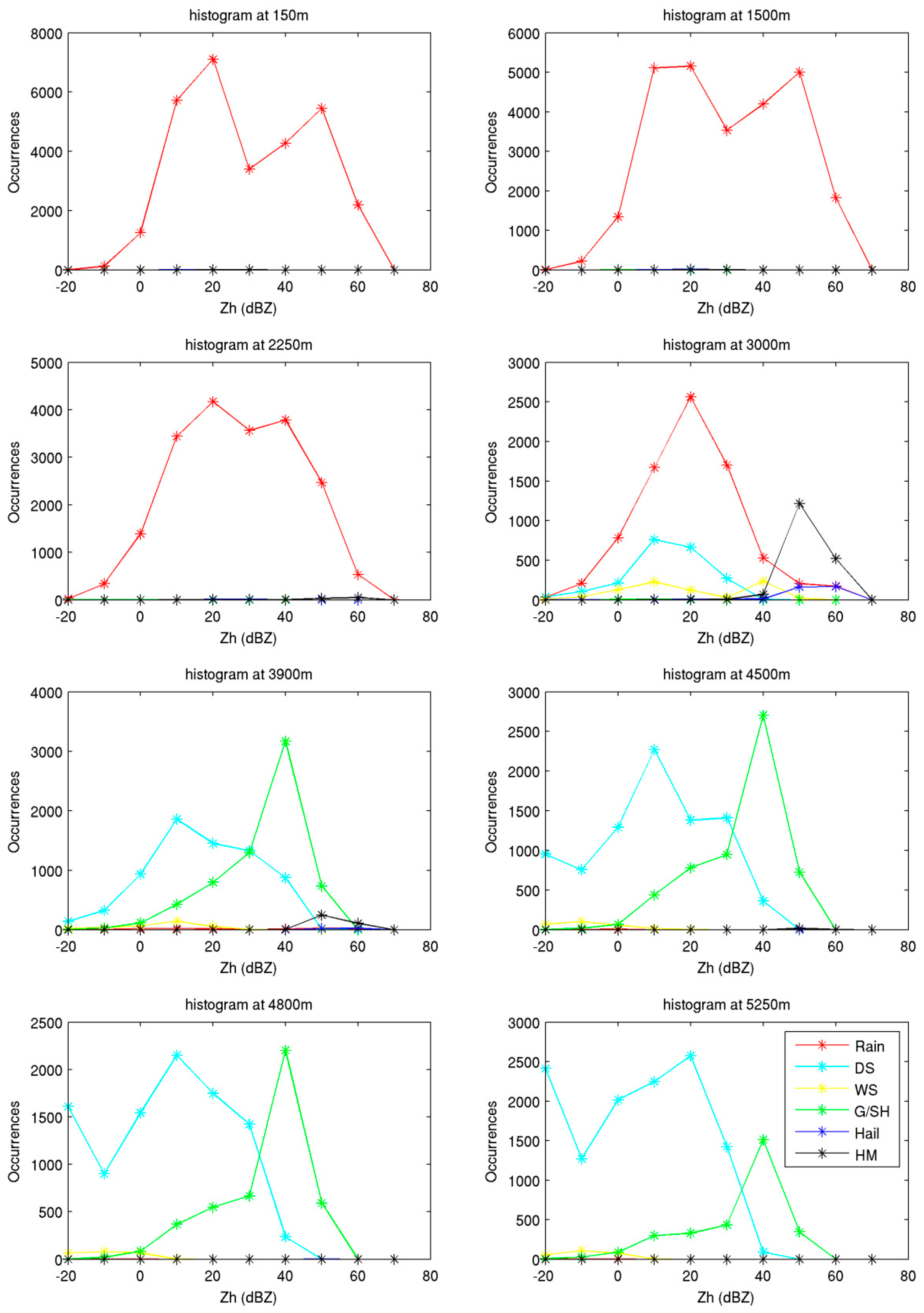
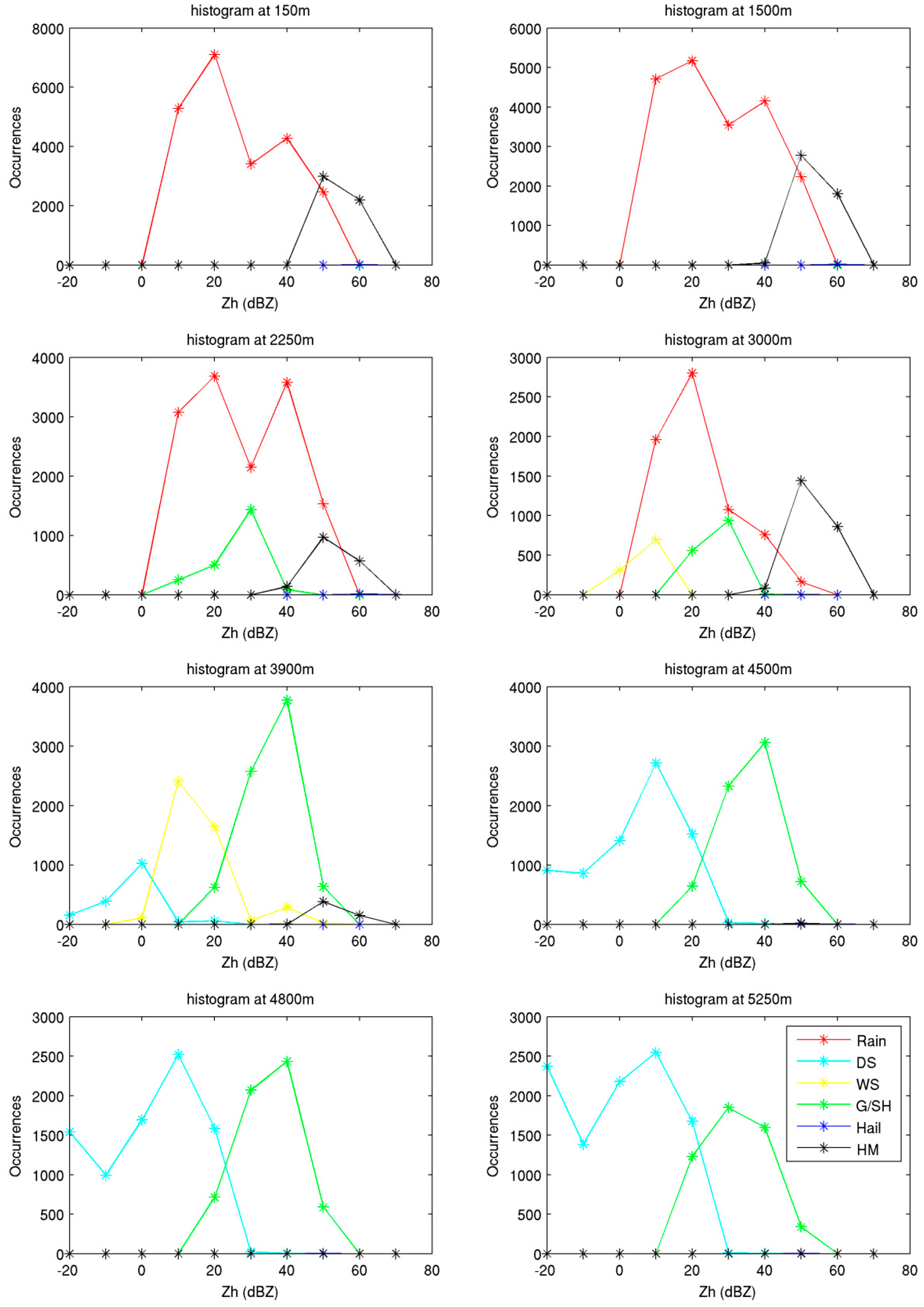
• Rain: this class includes, light rain, moderate rain and heavy rain (characteristics of convective events). For this reason, Z_h spans from 10 to 60 dBZ and Z_dr assumes positive values due to the oblate shape of rain. The liquid hydrometeors are typically detectable below the melting layer (ML).
• Dry Snow: this class includes all the non-wet ice particles, such as aggregates, plates, and columns, which determine the relatively low values of Z_h. Such particles are typically detectable above the ML.
• Wet Snow: this class typically refers to ice particles in the melting phase, which typically present in the ML. These hydrometeors are usually ice particles or aggregated ice particles covered by a film of water that result in high values of Z_h.
• Graupel: these hydrometeors are detectable both above and within the melting layer: usually these particles melt below the ML, but they may reach the ground during convective events with intense downdraft. They are smaller than hail and thus are associated with Z_h values lower than those found in hail. They produce Z_dr levels around 0, but conical graupel can produce negative Z_dr values.
• Hail: the presence of hailstones characterizes convective events. They are typically found in the core of the deep convective cells and are detectable from the ground up to several kilometers above the ML. The updraft of the convective cell drives the growth of these particles, whose dimensions can reach the order of centimeters. Hailstones have high variability in their size and shape distribution. A typical signature of these particles is high values of Z_h and Z_dr and K_dp values around 0 (due to tumbling).
• Hail Mix: these hydrometeors occur from ground to few kilometers above the ML. The hydrometeors in this class are representative of a mix, present within the radar resolution volume, of raindrops lifted by updraft, supercooled raindrops, hail, small hail, and graupel. The typical signature is high values of Z_h and low values of ρ_hv (these values decrease for the increase of hail amount of different size and increases with increasing mixing) while Z_dr spans from negative to positive values.

Since the training phase of the SVM is the core of the HCA set-up, the training set should be as representative as possible of the physical phenomena to be classified. For this purpose, a large number of cases, including different types of meteorological events, have to be included in the training set. The given set of available weather radar observations is divided into two subsets: the first is selected to perform the training phase, namely training observations (l), while the other one consists of the test observations (m).

A few processing steps are necessary to run both the SVM and FL HCAs:

• Unreliable data removal. pixel affected by ground clutter, anomalous propagation, and non-meteorological targets were identified and removed by applying a set of thresholds on Z_h and on the standard deviations of φ_dp and Z_dr [28].
• Estimation of specific differential phase. Different methods are used to estimate K_dp from differential phase shift measurements. For C-band datasets, K_dp is estimated using the finite difference method [28], while for X-band datasets an iterative moving-window range scheme was adopted [29].
• Attenuation correction for Z_h and Z_dr. Measurements propagated along paths below the 0°C level are corrected using a linear relation of K_dp with specific attenuation and specific differential attenuation (A_h, A_dp, respectively) i.e., A_h,dp = γ_h,dpK_dp. The parameterizations adopted to obtain γ_h,dp coefficients at X-band and C-band are performed by T-matrix scattering simulations using three years of disdrometer observations collected in Rome by a disdrometer [30].
• Correction of polarimetric variables for elevation angle. The values of the polarimetric variables of the same ensemble of scatterers change with the elevation angle. The most affected are Z_dr and K_dp, while Z_h typically does not change more than 1 dBZ, which is the intrinsic uncertainty due to noise. In general, Z_dr and K_dp exhibit their maxima at 0° elevation and their values gradually decrease to 0 when reaching vertical incidence. In this work, Z_dr and K_dp are corrected for elevation angles by recalculating their values as observed at 0° of elevation [31].
• Estimation of 0 °C level. The 0 °C level is estimated using vertical profiling soundings from the closest sounding station. If the processing is referred to the AWR, this level can be estimated directly from measurements collected by devices on-board an airplane.
• Input SVM data organization. The dual-polarization measurements Z_h, Z_dr, K_dp, and ρ_hv (or σ(Ф_dp) at C-band) and the height of 0° level are stored in an organized structure. The organization for the data access is made by n-tuples (a row of the whole structure contains a single n-tuple of polarimetric features).

The SVM algorithm is trained on classification maps generated by a FL classification approach. For each class the SVM descriptors (organized in the so-called support vector, SV) are extracted. In the case of operational classification, on the ground or during flight, the training is performed off the processing chain. Before performing the training procedure, input data are prepared. A training set is made up of a certain number (l) of n-tuples, depending on the accuracy needed by the user and on the related computational load (the higher the number of n-tuples, the more time required by the training phase). Furthermore, the data are scaled into a specific range. This step is necessary because, in general, the input features contained in each n-tuple may have values of different scales and therefore are not commensurable. The scaling of the data is performed on the test set as well as on the training set.

Furthermore, for nonlinear SVM using RBF kernel, the penalty parameter, C, and the kernel parameter, γ, need to be estimated. These parameters determine the capability of the algorithm to separate the hyperplanes. The better these parameters are identified, the more accurate is the prediction of the classifier. The identification of the best C and γ is performed during the training phase using a cross-validation (CV) procedure, a standard technique to adjust the parameters of prediction algorithms (details of this procedure are shown in Section 3.2). The SVM model, if trained on a large set of “representative” events, can be used to classify any set of data since its training can reach a high level of reliability. The results are used to configure the SVM model.The SVM model retrieved in the previous step is used to classify the whole dataset, providing as output a label for each n-tuple of input. In this way, a label is associated with each radar sample, providing the spatial distribution of the hydrometeors that build up the weather phenomena occurring in a specific geographical area.

3. SVM HCA Validation Using a Simulated Scenario

In general, it is very hard to get appropriate simultaneous measurements for physical validation of HCAs, while the microphysical output of a numerical weather model allows the straightforward evaluation of the capability of the HCA of interpreting the input radar variables to find the most probable hydrometeor class. In this section, the validation of the SVM algorithm using a synthetic set of measurements is shown. After having introduced the weather scenario and the radar simulated variables, the algorithm performances are evaluated in terms of accuracy of the prediction of the hydrometeor classes. First, the ability of SVM to find the correct parameters by varying the size of the training set is presented, then the results of the physical validation based on WRF outputs are shown in terms of confusion matrix.

3.1. Set-Up of a Weather Scenario and Simulation of Radar Observations

The Weather Research and Forecasting model (WRF) is used to provide a set of microphysical descriptors from which the radar observables are extracted. WRF model implementations exist at different temporal and spatial resolution. In this work, the non-hydrostatic model at the horizontal resolution of 1–3 km, able to simulate moist convection and advanced microphysical processes, is used [32]. The WRF loads the General Regularly-distributed Information in Binary form (GRIB) file describing a meteorological event chosen by the user and generates a synthetic 3D scenario providing several meteorological parameters in output (e.g., pressure, wind, temperature, moisture). Using the Millbrandt–Yau two-moment microphysics option [33,34] in WRF, microphysical parameters such as the mixing ratio (q, in kg·kg⁻¹),which is the ratio of the water vapor mass to the mass of dry air, and the concentration of particles (N_T, in m⁻³), can be obtained. Each microphysical parameteris available for four different classes of hydrometeors: rain, snow, graupel, and hail. The WRF outputs are used to generate microphysical parameters and, in combination with the T-matrix code, the corresponding scattering and propagation characteristics are obtained. In particular, in order to set the T-matrix simulation for each hydrometeor class, WRF outputs (wind fields, temperature, and microphysical parameters) have been used to define the size distributions of the particles and the probability density function of the aspect angle and the canting angle. Details on the use of WRF microphysics and additional assumption for running T-matrix are found in [20]. T-matrix provides the covariance matrix of the voltages at the radar receiver for each hydrometeor type from which polarimetric radar parameters can be obtained. Since each element of the WRF volume can contain a mixture of hydrometeors, the sum of individual voltage covariance matrix of the separate components is calculated [28]. This means that the different types of hydrometeors contribute separately to the covariance matrix, and the contributions of the covariance matrices of the different hydrometeor types can be added together to build the bulk covariance matrix.

A problem in training and testing the HCA using WRF outputs is that there are just four hydrometeor classes available from WRF, while for HCA there are sixclasses.

In this work, the classes of WRF are determined using the mixing ratio q in each volume, as shown in

Table 1. Hydrometeor Classification Algorithms (HCA) classes determined by values of q obtained from the WRF model. The percentages are the mixing ratio quantity of a given hydrometers with respect to the sum of q of all classes. DS stand for dry snow, WS for wet snow, and HM for hail mix. For instance, the rain class is defined when the percentage of q_rain is greater than 90%, while WS class is defined when q_rain is greater than 30% and q_snow is greater than 60%.

	Rain	DS	WS	Graupel	Hail	HM
qrain	>90%	0	>30%	0	0	>30%
qsnow	0	>90%	>60%	0	0	0
qgraup	0	0		>90%	0
qhail	0	0		0	>90%	>60%

. To obtain the six HCA classes, some were generated by mixing two separate WRF classes. Differences are in the snow class (HCA splits snow in two classes: wet snow and dry snow), and in the hail mix class (this class is present only in HCA and it is a mixture of rain and hail). This classification will be referred to as WRF-class the following.

The intense precipitation event that occurred on the afternoon of 15 October 2012 in the Southern Mediterranean and off the coast of Tunisia is selected as the test case to run the WRF model. The WRF scenario selected is composed of a cubic volume of 800 × 682 × 52 elements, whose resolution is 300 m × 300 m × 150 m, the last being the vertical resolution. WRF provides for each element of the cube and for each hydrometeor class the microphysical characteristics (q and N_T), and the meteorological variables (pressure, temperature, wind speed, and direction). Using the T-matrix code, the polarimetric radar parameters are calculated for each element of the WRF scenario. The polarimetric parameters obtained in this way are ideal values. In order to generate realistic polarimetric variables as would be measured by a real radar system, an error term simulating the effect of signal fluctuations is added. A radar system with a three-degree antenna beamwidth (a typical aperture of radar antennas mounted on civil aircrafts), operating at a frequency of 9.353 GHz, with a range resolution of 150 m has been assumed. Then, Gaussian distributed random variables have been added to ideal radar parameters obtained by WRF output. The standard deviations are set to 1 dB for Z_h, 0.2 dB for Z_dr and 0.01 for ρ_hv, while the K_dp standard deviation is calculated using the following formula [28]:

$$\sigma \left(K_{dp}\right)=\frac{\sigma \left({\mathsf{\Phi }}_{dp}\right)}{L}\sqrt{\frac{3}{\left[N-\left(\frac{1}{N}\right)\right]}}$$

(1)

where σ(Ф_dp) is the standard deviation of Ф_dp, fixed at 5°, L is the path length along which derivative estimation is performed, fixed at 1.5 km, and N is the number of range bins that are 10 in this case. The resulting value of σ(K_dp) is approximately 0.1° km^–1.

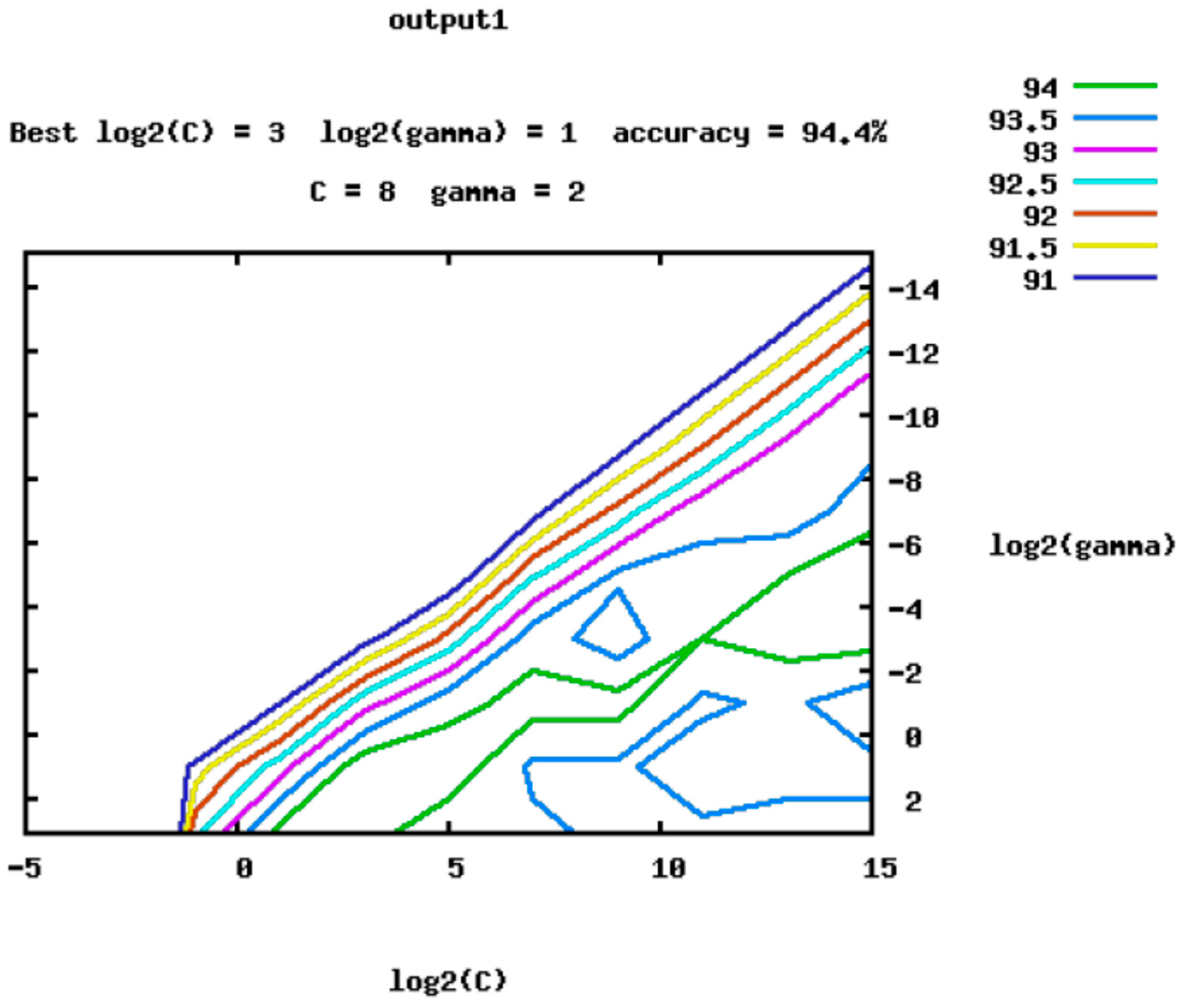
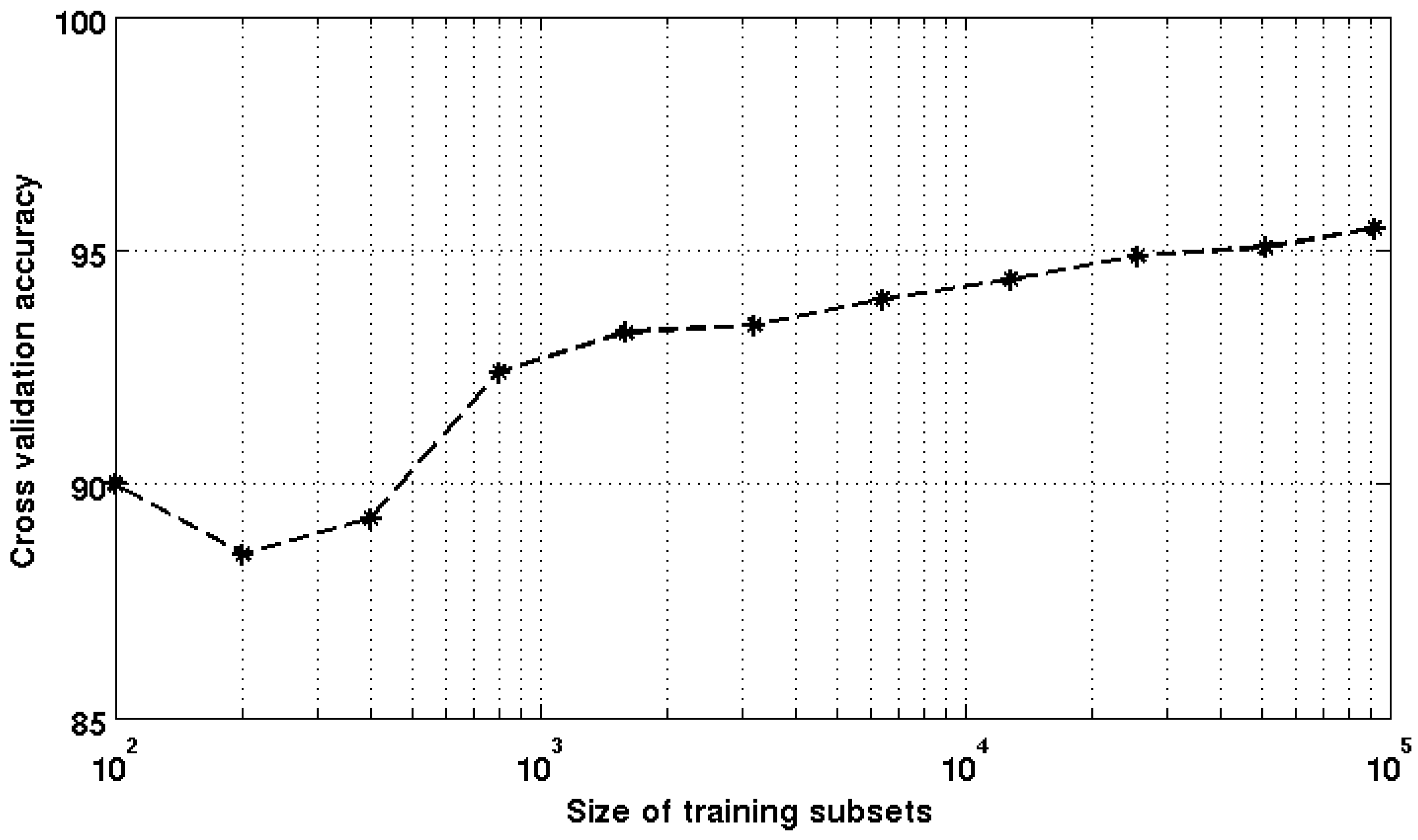
3.2. SVM Parameters Optimization

A SVM HCA algorithm has been implemented for the WRF scenario using realistic radar measurements (with noise added) and the height of 0 °C level given by the WRF model. The training set is obtained random sampling the elements of thevolume of data and includes 10⁵ samples, while a test set of 3 × 10⁶ samples (randomly sampled and excluding the samples belonging to the training set) was used to test the classifier. In order to get an estimate of SVM algorithm accuracy on predicting the membership functions of a certain class, typical steps are: (i) finding optimal tuning parameters; (ii) training a model using these optimal parameters on the full training set and (iii) testing this model on the test set. For the SVM scheme used in this work (with RBF kernel) the values of C and γ (see Section 2.1) need to be identified. It is not known beforehand which are the best values of C and γ for a given problem. A cross-validation procedure is used to get an accurate idea of the generalization error when certain tuning parameters are used, and an accurate CV can prevent the overfitting. A “grid-search “on C and γ using CV is performed: different pairs of (C,γ) values are tried and the one with the best CV accuracy is picked. To identify good parameters, a useful method is to try exponentially growing sequences of C and γ. Figure 1 shows the final grid plot of the grid-search process, in which a 94.8% accuracy was found for this SVM model for the best values C = 8 and γ = 2. In order to find how large the training set selected should be to achieve the desired degree of accuracy of prediction, the CV is performed at different size of the training set that varied from 10² up to 10⁵. Figure 2 shows that larger training subsets increase the CV accuracy, but also that when a certain size (in this case 10⁴) is exceeded, the CV accuracy does not increase significantly (the CV increase from 10⁴ to 10⁵ is around 1%): therefore, when this size is reached the code can be stopped. These processes demonstrate that 10⁴ observations are sufficient to train the SVM model with a high accuracy (94.8%) and in a reasonable processing time (less than 1 minute on an x86_64 Linux machine Eight core, Intel-i7@2,80GHz processor).

CV accuracy is a good measurement to optimize a SVM algorithm, but it does not allow us to evaluate whether all the classes in the training set are well represented by the SV. In fact, when the training is performed using random sampling, the classes that have low occurrences could not be sampled enough to establish a robust relationship. In order to allow adequate representation of all the classes in the model, the training set is quasi-equally dived among the classes. To assume such equiprobability of classes, the training set should be partitioned equally in to six classes. In this work, the maximum number of elements of the less numerous class is used to limit the number of element of each class that composed the training set.

3.3. SVM HCA Validation Using WRF Model Output

In addition to the performance of the SVM in separating hyperplanes, i.e., in finding the optimal parameters, we have also evaluated the classification results in terms of ability to identify hydrometeor classes.The validation of the classes predicted by the SVM with respect to the WRF microphysics expressed in terms of the q parameter (WRF-class) has been performed through the following method. The confusion matrix (CM) has been calculated between the truth and the predicted hydrometeor classes applied at the same test set. The element CM(i, j) contains the number of observations classified in the ith class, which in reality belong to the jth class. The diagonal contains the same classification for both algorithms (correct classification). Given the CM, the global performance of the SVM is quantified by the overall accuracy (OA), defined as

$$OA=\frac{{\sum }_{i=1}^{L}CM\left(i,i\right)}{m}\times 100$$

(2)

and the Cohen’s Kappa (K),

$$\mathsf{{\rm K}}=\frac{OA-P_e}{1-P_e}$$

(3)

where

$$P_e=\frac{{\sum }_{i=1}^L({\sum }_{j=1}^{L}C{M}_{j,i}{\sum }_{j=1}^{L}C{M}_{i,j})}{m^2}$$

(4)

where L is the total number of classes (L = 6) and m is the total number of observations. K takes into account the correct predictions that might occur by chance (P_e) and is a robust metric in the case of unbalanced classes.

In this study, the six classes of WRF-class are used to build up the microphysical validation set. The WRF scenario contains 2.8 × 10⁷ samples, each one associated to a vector of five elements (radar measurements and height), which implies a huge amount of data to be processed. In order to reduce the number of samples to be processed, and consequently, to reduce the computation time, 2 × 10⁵ elements are randomly extracted from the WRF cubic volume. A Monte Carlo method is applied to each sample of the subset in order to generate 100 sets of polarimetric variables, randomly extracting 100 realizations of a set of radar realistic variables and generating a dataset of 100 × 2 × 10⁵ samples. The dataset obtained by the Monte Carlo method is then used to implement the SVM model, splitting it in two sub-datasets, one for training (by extracting 10⁴ samples and respecting the equal distribution of samples among the six classes) and the other (consisting of the samples left) for testing. The SVM classification is applied to each set of random variables generating a synthetic dataset of 100 realizations. These synthetic scenarios allow us to estimate the confidence intervals (CIs, namely the 10th and 90th percentile) of the established metrics, calculating for each realization the CM and the respective OA and K coefficients. The CM with the CIs intervals is shown in

Table 2. Confusion matrix per class of the WRF scenario obtained by using 100 × 2 × 10⁵ observations for each realization (infinite values are excluded in the CM). For each element, the CIs intervals (found using, the 10th, 50th, and 90th percentiles) are shown. Classifications matched by WRF and SVM are found along the diagonal and misclassifications are in the off-diagonal entries.

	Model (WRF)
Predicted (SVM)		Rain	DS	WS	Graupel	Hail	HM
		51,390.0	1252.5	6289.0	567.0	210.0	913.5
	Rain	51,447.0	1275.0	6320.0	592.5	222.0	941.0
		51,511.0	1290.0	6351.0	610.5	231.5	967.0
		823.0	41,477.5	9689.0	5136.0	6.0	6.0
	DS	835.5	41,524.0	9702.5	5172.0	8.0	7.0
		852.0	41,585.5	9714.5	5209.0	10.0	9.0
		902.0	1940.0	2308.0	2382.0	13.0	172.0
	WS	917.0	1964.0	2327.0	2422.5	16.0	180.0
		935.5	1993.0	2345.0	2454.5	20.0	190.0
		4566.5	7401.5	916.5	17,119.0	2.0	17.0
	Graupel	4601.0	7457.5	951.0	17,168.5	4.0	22.0
		4648.5	7515.5	980.5	17,219.5	6.0	27.0
		1087.0	0.0	0.0	48.5.0	1311.0	1627.5
	Hail	1112.5	0.0	0.0	56.5	1352.5	1668.0
		1151.0	0.0	0.0	67.0	1407.0	1719.0
		7059.5	0.0	0.0	124.5	16,346.0	16,029.0
	HM	7106.5	0.0	0.0	135.0	16,396.0	16,082.5
		7144.5	0.0	1.0	147.0	16,443.0	16,120.0

. Main differences are found for wet snow and hail mix, that are additional to the four default classes of the WRF model. The wet snow class of WRF is distributed between rain, dry snow, wet snow and graupel, of SVM classes; the hail class of WRF is mostly associated with the hail mix of SVM class. Details on the radar dual-polarization signatures of WRF-class classes comparing to HCA classes are presented in Appendix B.

In spite of the differences between the WRF and SVM classes, good performances are obtained for SVM classifications using the metric described above and calculating the respective CIs. The CI found for the OA is [64.89 64.95 65.02]% and for the K is [0.5506 0.5513 0.5522]. CIs are very narrow, meaning that measurement errors do not impact on classification results. Moreover, results obtained from the comparison between WRF microphysics and SVM HCA using CM highlight that SVM model gives a fairly good prediction of WRF classes via the FL training set. More results relative to SVM classification performance are shown in Section 4, describing the behavior of the SVM HCA applied to real datasets.

The structure of the SVM is easily reconfigurable: it possible to train the algorithm using any type of adequate validation dataset available. For hydrometeor classification purposes, different data sources can be investigated to train the algorithm, such as different Numerical Weather Prediction model outputs or other sensor information, e.g., disdrometer measurements [15].

4. Evaluation of the SVM Hydrometeor Classification with Real Measurements

The SVM model presented in Section 2 has been applied to measurements collected by X- and C-band ground based systems. Two datasets have been analyzed: one includes measurements collectedon 2013 by an X-band dual-polarization Doppler radar operating within Catania airport, and the other includes measurements collected on 2012 and 2015 by the Polar 55 C, C-band dual-polarization Doppler located in Rome. The training phase was implemented with the support of the fuzzy logic classification scheme according to the approach explained in Section 2.2.

4.1. C-Band Dataset

Sixteen intense precipitation events that occurred over Central Italy in September–October 2012 during the Special Observation Period 1 (SOP1) of the Hydrological cycle in Mediterranean Experiment (HyMeX) and an event that occurred on 12 October 2015 [9,35] were selected to evaluate the SVM HCA algorithm. Although these events have predominantly convective characteristics, they include parts during which the precipitation was less intense and exhibit stratiform characteristics. These events were observed by the Polar 55C radar located in Rome (latitude: 41.842° N, longitude: 12.646° E, 132 m above sea level) at ISAC-CNR. Polar 55C is a research-grade C-band (5.6 GHz frequency) Doppler dual polarization radar (details of the system characteristics can be found in [36]). The data selected were collected with a volume scanning composed of 7 or 8 Plane Position Indicator (PPI) at different elevations (from 0.6° to 12°) performed every 5 min. In addition, some sweeps along the vertical were performed for Z_dr calibration and for detailing the vertical structure of precipitation. Moreover, sweeps at fixed azimuths with varying elevation (Range Height Indicator, RHI) were also performed to scan the most intense convective cells. The range resolution was 75 m, corresponding to a pulse duration of 0.5 μs. The pulse repetition frequency was 1200 Hz while the maximum range was limited to 120 km. To test the classification performance, the SVM HCA was applied to all the volume scans (in total 1257 volumes consisting of 7–8 PPIs depending on the case study) and the 33 RHI scans (in each map 360 × 1600 samples). Data were corrected for attenuation due to propagation as described in Section 2.2. The training set was obtained by a random selection of 100 volumes classified by the FL scheme that contains different type of precipitation regimes (convective and stratiform). After the random selection, a human inspection on the 100 volumes was made in order to check that these volumes include both convective and stratiform precipitation regimes (at least 20% and 80%). Finally, from these datasets 10⁴ samples (not empty) were randomly extracted (respecting the equipartition of sampled per the class) to build the training set.

4.2. X-Band Dataset

The case studies considered occurred on 21 February and 21 August 2013 in Sicily and were observed by the Selex-Gematronik 50 DX system (with a 3 dB antenna beamwidth of 1.3° and a transmit peak power of 50 kW) of the Department of Civil Protection of Italy, operational at the airport of Catania [27]. The radar performed a volume scan made of 12 sweeps at different antenna elevation angles ranging from 1° to 21.6°, and an additional one at vertical incidence. The range resolution was 200 m and the maximum unambiguous range was 80 km, corresponding to a PRF of 1875 Hz. The dataset consists of 19 volumes collected during the intense part of the 21 February event and 55 volumes during the 21 August 2013 event. Each radar volume contains 1.7 × 10⁶ samples. As demonstrated in Section 3.2, 10⁴ samples are sufficient to train the SVM model. Ten radar volumes among the 74 available were selected for the training phase (and excluded from the test set), from which a subset of 10⁴ samples was obtained by a random selection respecting the equipartition of samples per class.

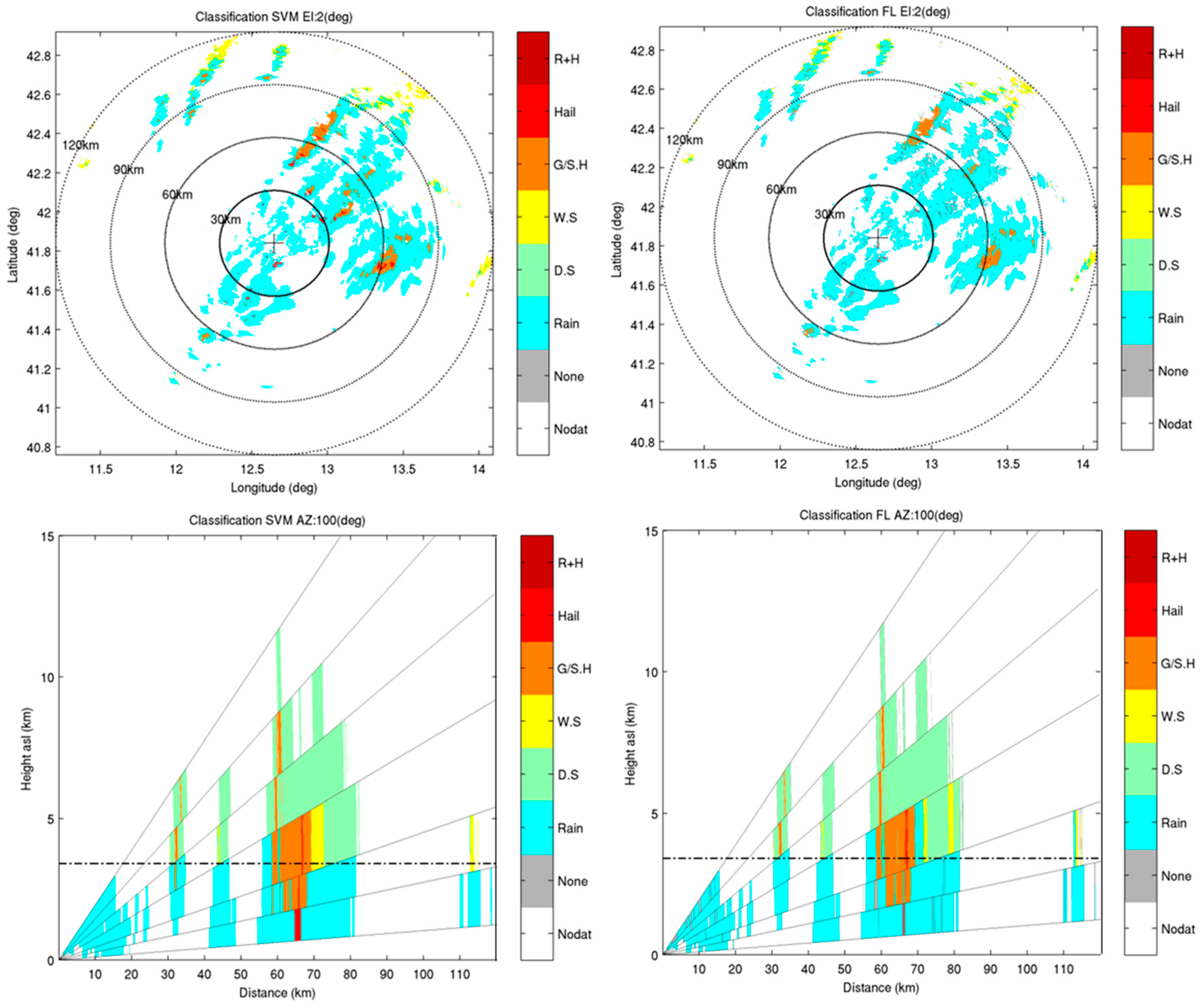
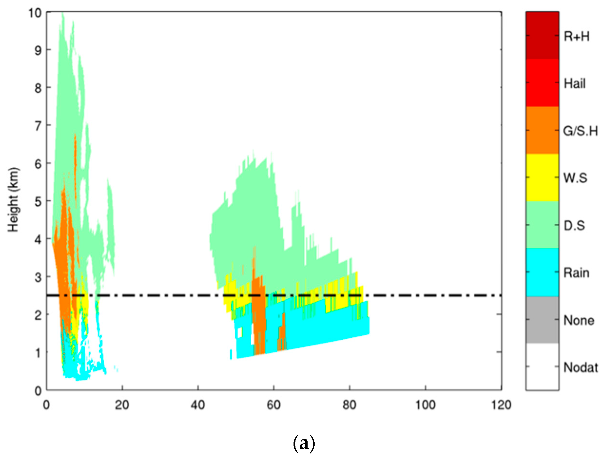
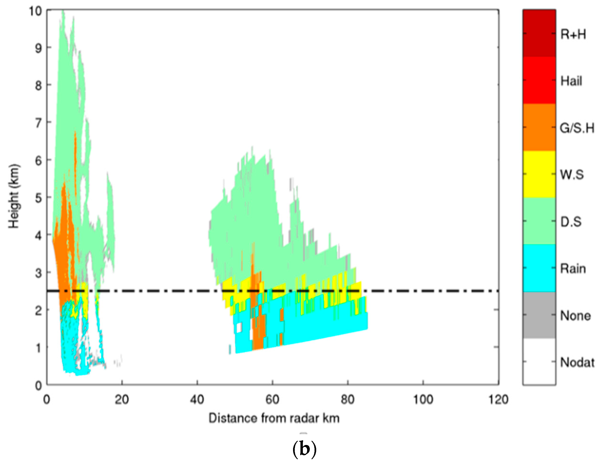
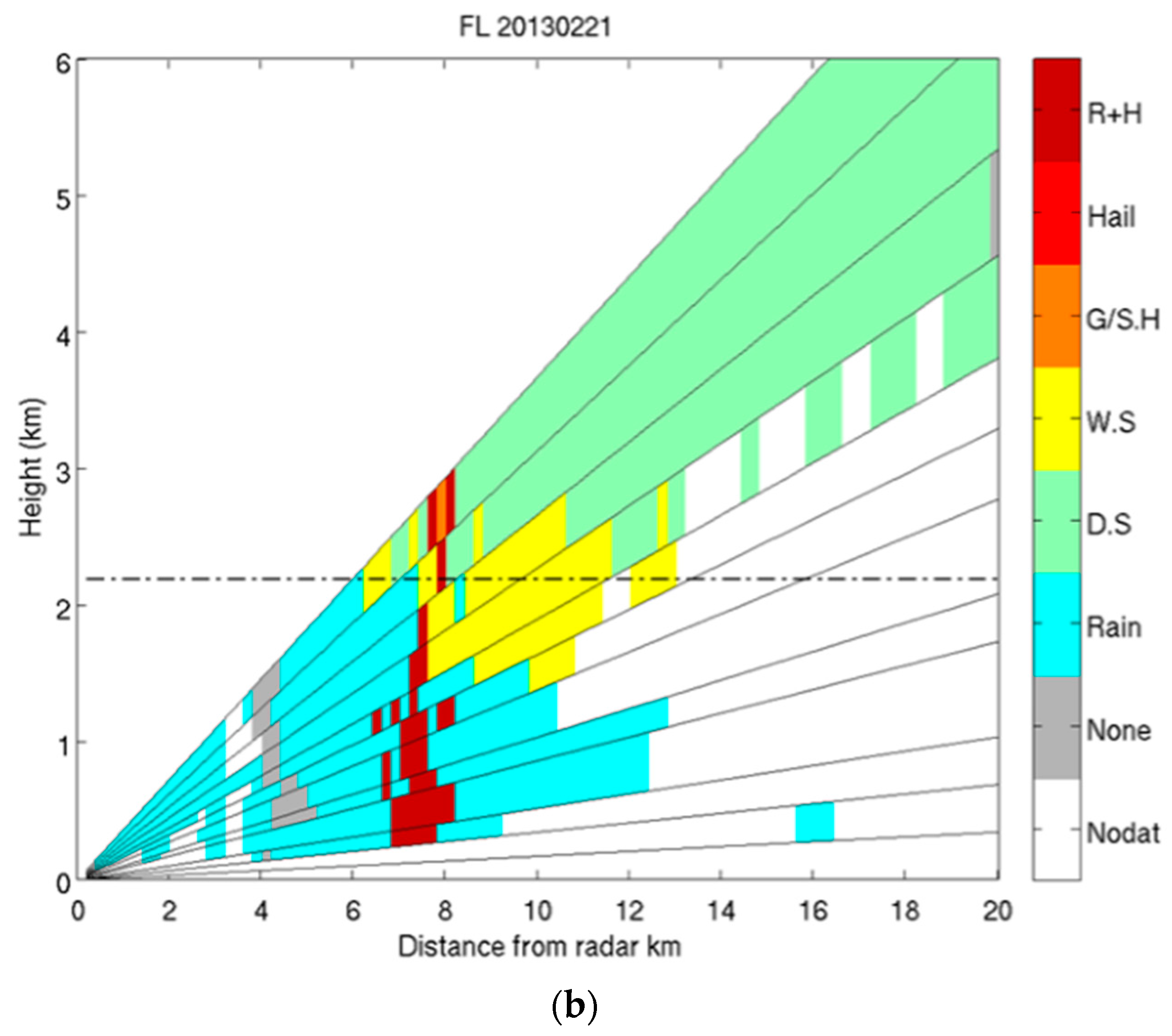
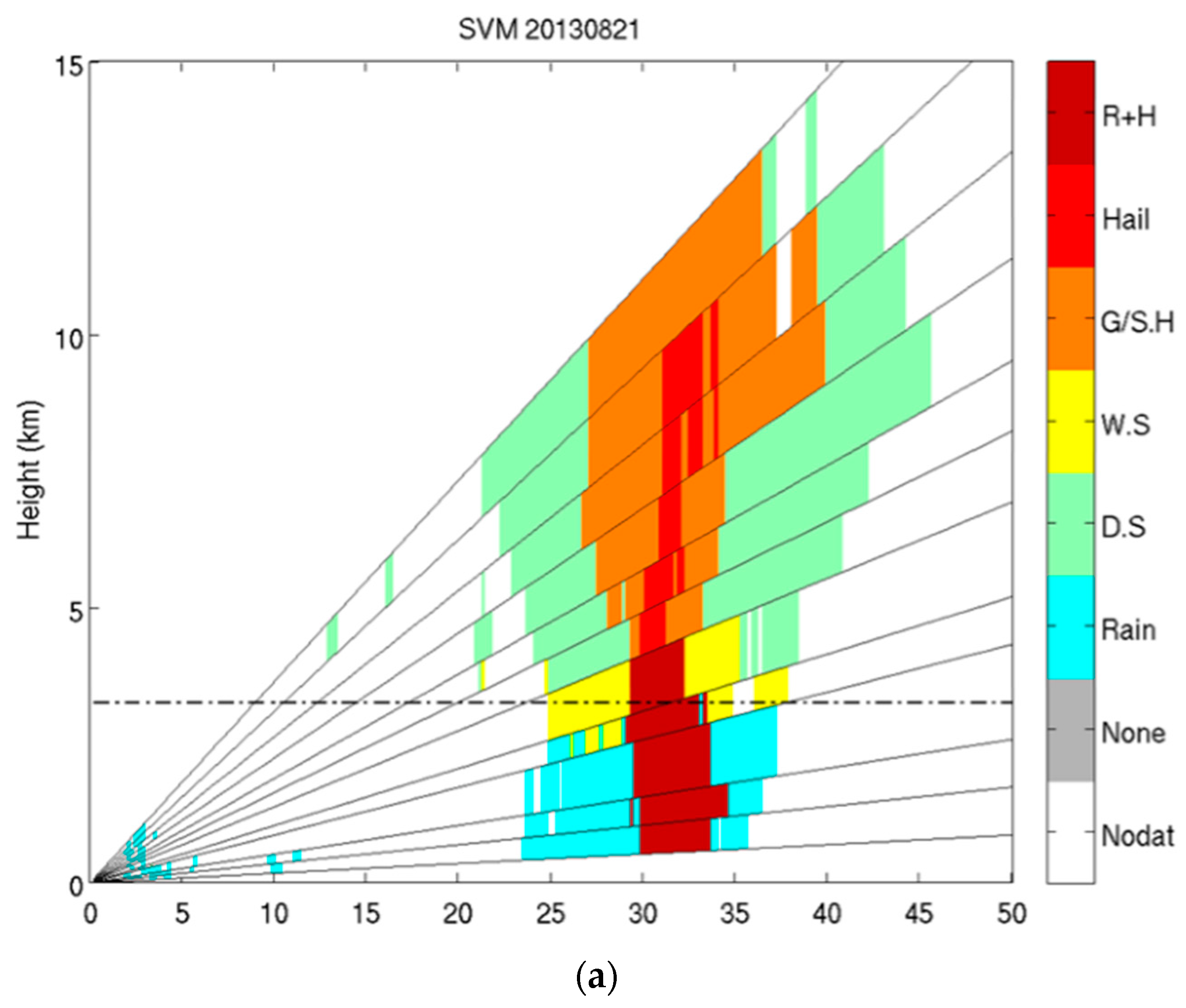
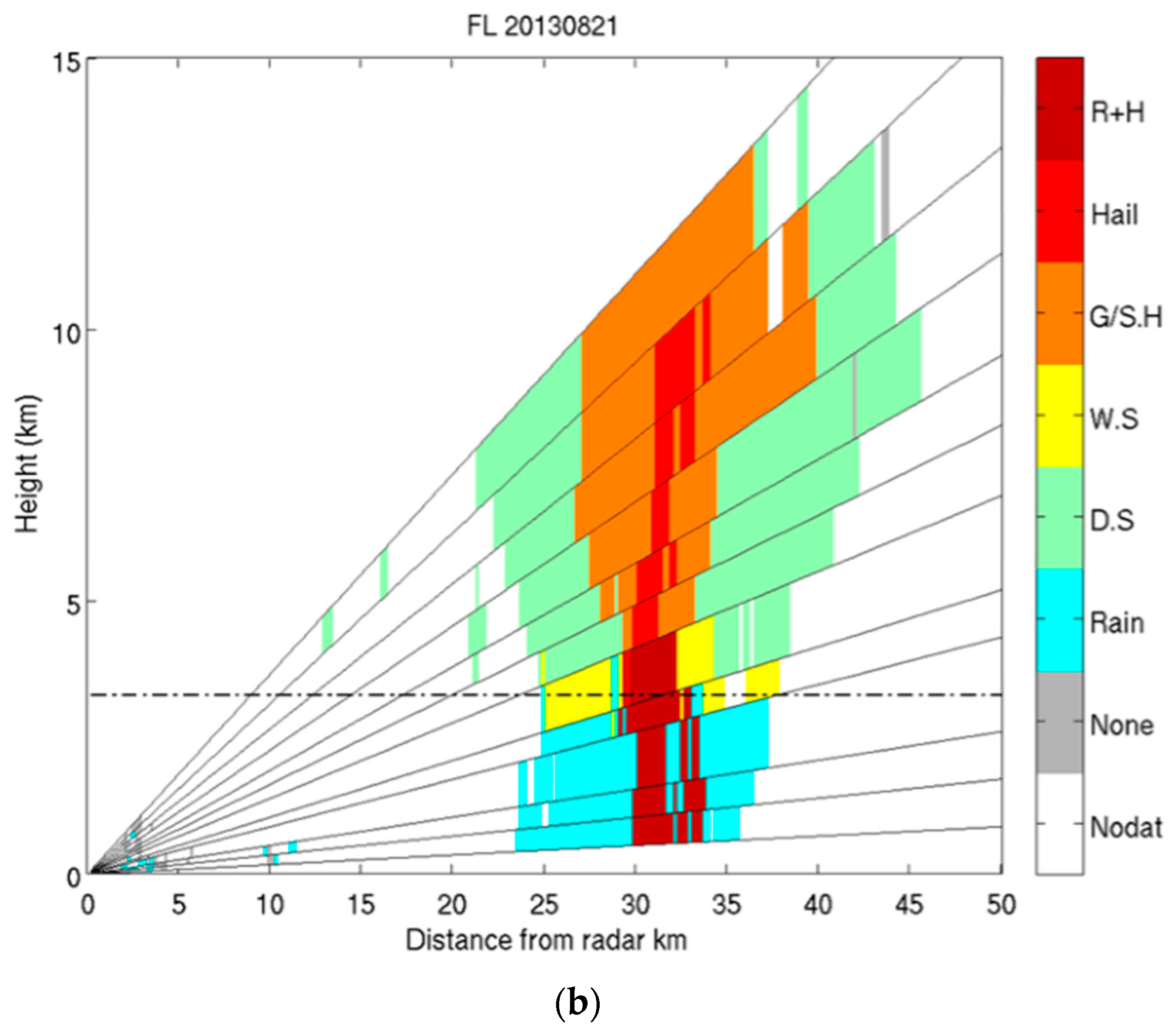
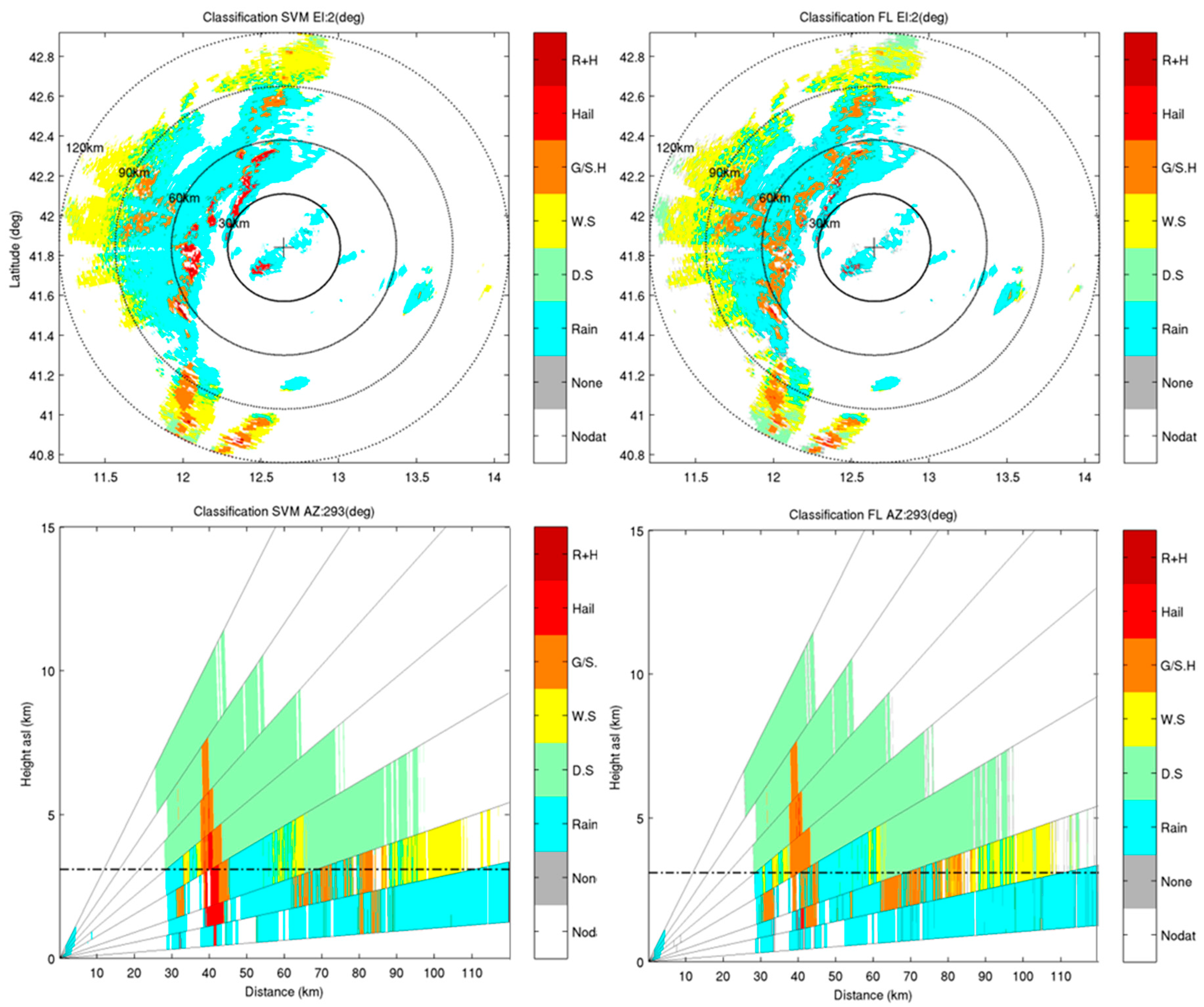
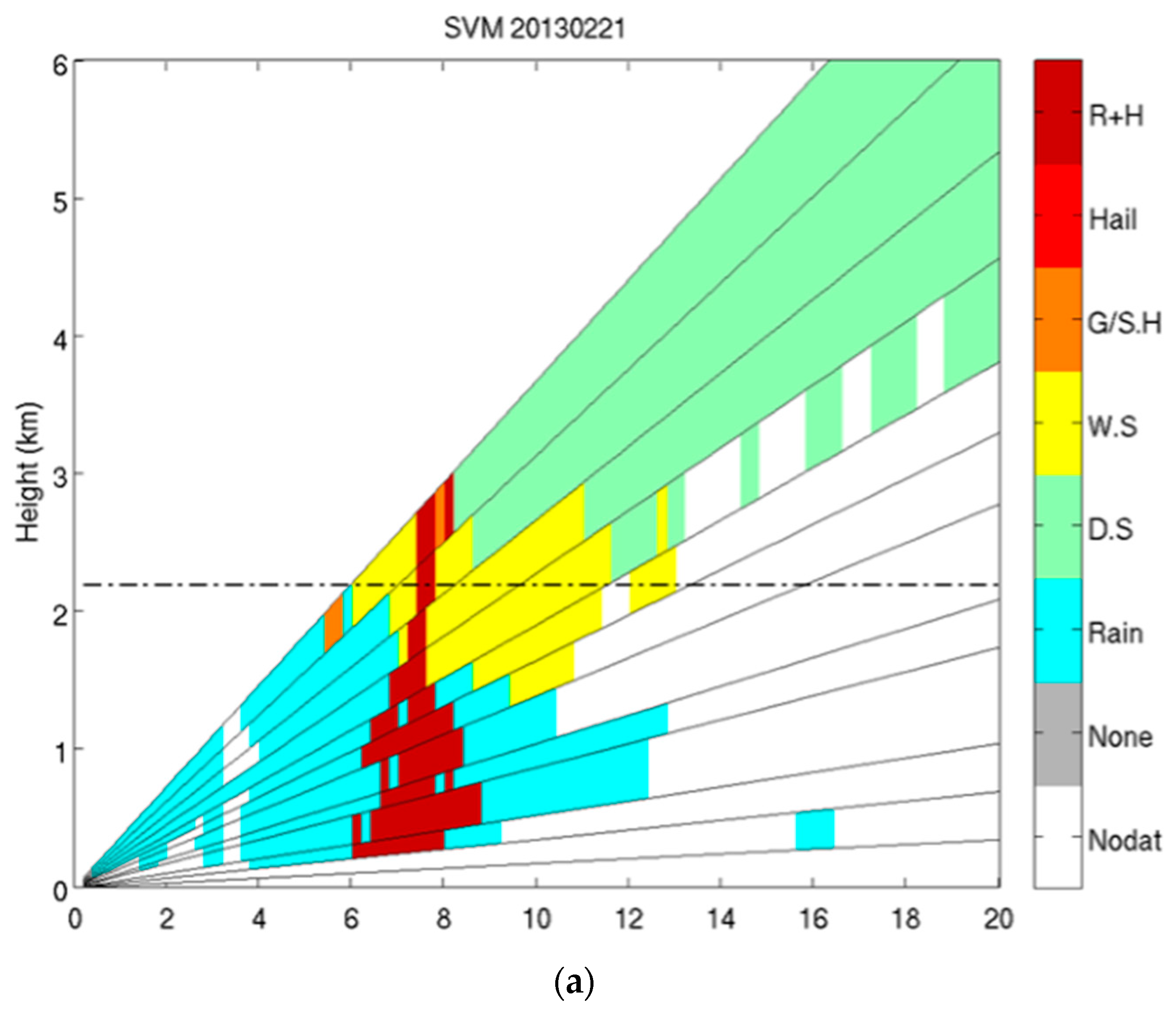
4.3. Comparison of Results from SVM and FL Classification

In order to evaluate the performance of SVM model with real data, qualitative and quantitative comparisons with output provided by the FL classification are discussed in this section. SVM classification results applied to Polar 55C quasi-horizontal sweeps are shown in Figure 3 and Figure 4 for two volumes collected on 15 October 2012 and 12 October 2015 during intense precipitation. Upper panels show a PPI presentation of the classification results pertinent to data collected at 1.6° elevation, while bottom panels show the pseudo RHI reconstructed from volume data along specific rays. The output of the SVM (panels in left column) is compared, for the same data, with the output of the FL classifier (panels in right column). At first glance, the results do not differ much from each other, as expected. However, it can be noticed that the SVM classifier is able to classify data that are not classified (labeled as “None” and plotted in gray) by the FL classifier. In fact, the last stage of FL process consists in assigning a class based on rule strength. If it falls below a certain threshold [28], a pixel is labeled as not classified, while the SVM model always assigns a class label to a set of radar measurements. Furthermore, the SVM output appears more homogeneous and less noisy than the FL output. For example, the graupel area detected by the SVM shown on the pseudo RHI of Figure 3 (left panel) is less fragmented than the corresponding area classified by the FL (right panel). Nevertheless, since both classification approaches are applied on a point-by-point basis, such results can be attributed to the ability of SVM to learn from the entire hyperspace of radar measurements and to the accurate training of the model that includes high number of maps used (i.e., each class is assigned by SVM HCA based on relations obtained combining in several ways polarimetric radar variable). More impressive is the performance of SVM applied to the data shown in the RHI plots of Figure 5, where spatial homogeneity and spatial coherence are more evident with respect to the classification map obtained with the FL. Two convective cells are well distinguished, the first one close to the radar (at less than 20 km) and extended up to 8 km height, and the other one at around 50 km of distance, reaching 5 km height. Both cells are characterized by a core of graupel and rain close to ground, but the SVM classifier (upper panel) well identifies these cells detecting homogenous graupel region, while the FL classification (bottom panel) of these cells is fragmented in non-identified and spurious hydrometeors types. Figure 6 and Figure 7 show the pseudo-RHI for the two X-band case studies classified using SVM model (Figure 6a and Figure 7a) and FL schemes (Figure 6b and Figure 7b). Even at X-band, it can be noticed that the SVM classification results appear more spatially homogeneous in terms of image texture.

Besides the qualitative comparison between classification maps, the SVM model performance can be objectively evaluated with respect to the FL classification. Since a “true” reference is not available, some quantitative indicators must be used. A number of quantitative indices have been calculated, such as texture image parameters, connected component labeling (CCN), and labels classified by SVM respect to unclassified by FL. The following parameters have been evaluated from the co-occurrence matrix considering horizontal neighboring resolution cell separated by distance 1, as illustrated in [37]:

$$Co\left(i,j\right)= {\displaystyle \sum }_m{\displaystyle \sum }_n\{\begin{array}{c}1, if I\left(m,n\pm 1\right)=i and I\left(m,n\right)=j\\ 0, otherwise\end{array}$$

(5)

where m, n are the position indices and i, jare the indices of the class values (from 1 to 6). The normalized co-occurrence matrix, N_d(i, j) is obtained dividing the Co matrix by the sum of its elements ${\sum }_n{\sum }_{m}Co\left(n,m\right)$. From N_d are derived:

$$Energy= {\displaystyle \sum }_i{\displaystyle \sum }_j{N}_d^2\left(i,j\right)$$

(6)

$$Entropy= -{\displaystyle \sum }_i{\displaystyle \sum }_j{N}_d\left(i,j\right){\log }_2{N}_d\left(i,j\right)$$

(7)

$$Homogeneity= {\displaystyle \sum }_i{\displaystyle \sum }_j\frac{N_d\left(i,j\right)}{1+\left|i-j\right|}$$

(8)

These features are frequently used to characterize images. Energy measures the textural uniformity, i.e., pixel pairs’ repetition, by detecting disorders in textures. High energy values occur when the class distribution has a periodic pattern. The entropy is a feature that measures the randomness of class distribution. The entropy is large when the image is not texturally uniform and Co matrix elements have very small values. Complex textures tend to have high entropy. Entropy is strongly, but inversely, correlated to energy. Homogeneity measures image homogeneity as it assumes larger values for small differences in pair elements. It is more sensitive to the presence of near diagonal elements in the Co matrix. It is at a maximum when all elements in the image are identical. In this work these indices are compared one to one for the same image in order to get information on possible improvement of SVM classifications in term of hydrometeor spatial coherence with respect to the FL classification. Energy and homogeneity are features that measure the uniformity of class distribution and their values are expected to be high. The spatial homogeneity is also assessed by the CCN technique. Given a map the number of connected region N_r(k), where k is the class label, are identified by the CCL algorithm [38] checking eight connections and the regions are sequentially labeled. A hydrometeor class can be considered spatially homogeneous when the CCL algorithm detects a low number of N_r(k) for that class. In this metric, when the two classification maps (SVM and FL) for the same scene are compared, the one that presents the smallest number of CCL, calculated by the index $S={\sum }_k{N}_r\left(k\right)$, is the one with the highest spatial homogeneity. Quantitative indices are calculated for corresponding classification map pairs.

Since RHI maps at C-band and volumes of PPI at X-band are of the order of tens, quantitative indices are calculated for selected maps. The SVM classification for the RHI map (upper panel in Figure 5) is clearly spatial homogenous and coherent with respect to the FL classification. These qualitative considerations are confirmed by good performances obtained by the quantitative indices listed in

Table 3. Quantitative indices for classification results obtained by the SVM and FL HCAs. Scores are referred to the C-band RHI shown in Figure 5.

	None	Energy	Entropy	Homogeneity	S
	20121015 1738UTC
SVM	0	0.424	0.369	0.957	281
FL	2404	0.341	0.365	0.893	323

. Quantitative indices for classification results obtained by the SVM and FL HCAs. Scores are referred to the C-band RHI shown in Figure 5. Major improvements are registered in terms of homogeneity and energy, while entropy does not vary. Despite the high number of CCL found in this scene, there are 42 CCL less in the SVM classification map than in the FL one and 2404 pixels not classified in the FL classification map are instead labeled by the SVM HCA. X-band scores related to the SVM classification for the two scenes shown in Figure 6 and Figure 7, exhibit slight improvements on all indices compared to the scores related to the FL classification (

Table 4. As in Table 3, scores refer to two X-band classification maps shown in Figure 6 (upper lines) and Figure 7 (lower lines).

	None	Energy	Entropy	Homogeneity	S
	20130821 0450UTC
SVM	0	0.255	0.951	0.977	29
FL	73	0.247	0.939	0.958	37
	20130221 1520UTC
SVM	0	0.333	0.689	0.952	17
FL	24	0.336	0.678	0.937	19

).

The number of test maps available for C-band is 1257, considering all the PPI scans in the volumes for all the case studies. In order to obtain a consistent statistical sample, 100 pairs of maps have been randomly extracted (without replacing samples) and the quantitative indices calculated comparing each couple of maps.

Table 5. Quantitative indices for classification results obtained by the SVM and FL HCA. The dataset consists of 100 PPIs collected by Polar 55C at 1.6° elevation angle extracted randomly from the entire dataset. The CIs for each index are derived from the 10th, 50th, and 90th percentiles are listed for each classification approach.

	None	Energy	Entropy	Homogeneity	S
SVM	0	0.645	0.105	0.933	87
	0	0.820	0.339	0.964	448.5
	0	0.981	0.784	0.996	1691.5
FL	900.5	0.414	0.102	0.790	77.5
	3062.5	0.663	0.334	0.861	473.5
	9527.5	0.790	0.776	0.917	2126

shows the CIs for each quantitative index, calculating the 10th, 50th, and 90th percentiles. The SVM classification exhibits good performances for all indices with respect to the FL classification. Noticeable are homogeneity scores: the SVM values are very close to one (the lower limit of CIs is 0.93 and the upper limit is 0.99). Furthermore, an index of low fragmentation texture of the maps is found in the SVM classification, where they exhibit a smaller CCL (448.5 at 50th percentile) with respect to the FL maps (473.5 at 50th percentile). Finally, 3062.5 non-classified pixels are found at 50th percentile inthe FL classification maps, which are instead assigned in the SVM classification maps.

5. Conclusions

A supervised hydrometeor classification approach based on a learning machine method, a Support Vector Machine, is presented in this work. The algorithm, after having established robust relations between input variables and known samples (training phase), is able to predict the membership class of an unknown sample (prediction phase). Input variables are four dual-polarization radar measurements and the height of the 0 °C level. Results obtained by a fuzzy logic HCA, one of the most used hydrometeor classification approaches based on empirical rules, have been used as reference to train the SVM algorithm.The challenging task of validation has been achieved with realistic scenarios generated by the numerical weather prediction model WRF. Validation skills in hydrometeor identification of the SVM algorithm have been evaluated by using the output of the WRF model in which microphysical scheme are explicit. Hydrometeor classification has been performed in each grid point of WRF in which microphysics characteristics, denoted by mixing ratio for four hydrometeor class, were known. Six hydrometeor classes that include two additional classes with respect to WRF scheme (obtained by mixing two classes) have been derived by quantifying the mixing ratio. From the WRF model outputs, realistic polarimetric radar measurements were simulated by using the T-matrix code and adding random errors to each radar variable. The HCA-SVM classification and the WRF outputs were compared (on 2 × 10⁵ samples of the WRF scenario) by calculating a confusion matrix matching the six hydrometeor classes: good performances were obtained finding 65% of overall accuracy and 0.55 of Cohen’s coefficient.

The HCA algorithm has also been applied to real radar measurements collected by two ground based radar systems at X- and C-band. Two case studies occurred during 2015 in Sicily were observed by the X-band dual polarization Doppler radar located at Catania’s airport, while several observations were made in Central Italy during 2012 and 2015 by the C-band dual-polarization Doppler radar located in Rome at ISAC. Data collected using scanning modes (PPI volumes and RHI) were included in the dataset. The SVM algorithm has been trained by randomly sampling a part of the dataset and the rest part was used as test. To evaluate the SVM classification results, operational classification product obtained by using the FL approach has been applied to the same dataset. Qualitative comparisons between FL and SVM classification maps have revealed several positive features of the SVM classifier: (i) the texture of the maps is more homogeneous and less noisy; (ii) the maps appear more spatially coherent and homogeneous; and (iii) pixels not classified by the FL classification are classified by the SVM in a manner that appears consistent with the classes of the neighboring pixels. In order to quantify these SVM skills, some quantitative indices, mainly related to textural analysis, have been calculated for each pair of classification maps. Such a quantitative analysis has confirmed the benefits conferred by the SVM classification. In particular, RHIs classification maps have shown the highest scores: energy and homogeneity have increased of 20% and 10%, respectively, and more than 2400 not classified pixels have been assigned to a hydrometeor class by SVM HCA. Thanks to a large availability of PPI volumes at C-band (1257 volumes), a dataset of 100 maps has been selected and quantitative indices calculated at the 10th, 50th, and 90th percentiles. Indices related to texture analysis of image, energy and homogeneity, increased around 21% and around 12% (at the 50th percentile), respectively. The improvements found by SVM classifier with respect to FL, even though both classification approaches are applied pixel-by-pixel, can be attributed: (i) to thousands of pixels classified by SVM (not classified in FL); (ii) to the ability of SVM to learn from the entire hyperspace of radar measurements and (iii) to the accurate training of the model, which includes a large number of maps.

Besides the good performance of SVM in terms of hydrometeor identification shown in this work, the SVM approach has also exhibited a superior computational efficiency with respect to the FL approach. This suggests the possibility of using the SVM HCA in quasi-real-time tasks, as could be required by avionic applications running on devices that process radar measurements collected during the flight, with the purpose of avoiding areas characterized by hazardous weather.

References

1. Liu, H.; Chandrasekar, V. Classification of hydrometeor type based on multiparameter radar measurements: Development of a fuzzy logic and neuro fuzzy systems and in-situ verification. J. Atmos. Ocean. Technol. 2000, 17, 140–164. [Google Scholar] [CrossRef]
2. Straka, M.; Zrnic, D.S.; Ryzhkov, A.V. Bulk hydrometeor classification and quantification using polarimetric radar data: Synthesis of relations. J. Appl. Meteorol. 2000, 39, 1341–1372. [Google Scholar] [CrossRef]
3. Dolan, B.; Rutledge, S.A. A theory-based hydrometeor identification algorithm for X-band polarimetric radars. J. Atmos. Ocean. Technol. 2009, 26, 2071–2088. [Google Scholar] [CrossRef]
4. Dolan, B.; Rutledge, S.A.; Lim, S.; Chandrasekar, V.; Thurai, M. A robust C-band hydrometeor identification algorithm and application to a long-term polarimetric radar dataset. J. Appl. Meteorol. Climatol. 2013, 52, 2162–2186. [Google Scholar] [CrossRef]
5. Zrnić, D.S.; Ryzhkov, A.; Straka, J.; Liu, Y.; Vivekanandan, J. Testing A Procedure for Automatic Classification of Hydrometeor Types. J. Atmos. Ocean. Technol. 2001, 18, 892–913. [Google Scholar] [CrossRef]
6. Marzano, F.S.; Scaranari, D.; Vulpiani, G.; Montopoli, M. Supervised classification and estimation of hydrometeors using C-band dual-polarized radars: A Bayesian approach. IEEE Trans. Geosci. Remote Sens. 2008, 46, 85–98. [Google Scholar] [CrossRef]
7. Al-Sakka, H.; Boumahmoud, A.A.; Fradon, B.; Frasier, S.J.; Tabary, P. A new fuzzy logic Hydrometeor Classification Scheme applied to the French X-, C-, and S-band polarimetric radars. J. Appl. Meteorol. Climatol. 2013, 52, 2328–2344. [Google Scholar] [CrossRef]
8. Thompson, E.J.; Rutledge, S.A.; Dolan, B.; Chandrasekar, V.V.; Cheong, B. A Dual-Polarization Radar Hydrometeor Classification Algorithm for Winter Precipitation. J. Atmos. Ocean. Technol. 2014, 31, 1457–1481. [Google Scholar] [CrossRef]
9. Roberto, N.; Adirosi, E.; Baldini, L.; Casella, D.; Dietrich, S.; Gatlin, P.; Panegrossi, G.; Petracca, M.; Sanò, P.; Tokay, A. Multi-sensor analysis of convective activity in central Italy during the HyMeX SOP 1.1. Atmos. Meas. Technol. 2016, 9, 535–552. [Google Scholar] [CrossRef]
10. Bechini, R.; Chandrasekar, V. A semisupervised robust hydrometeor classification method for dual-polarization radar applications. J. Atmos. Ocean. Technol. 2015, 32, 22–47. [Google Scholar] [CrossRef]
11. Grazioli, J.; Tuia, D.; Berne, A. Hydrometeor classification from polarimetric radar measurements: A clustering approach. Atmos. Meas. Tech. 2015, 8, 149–170. [Google Scholar] [CrossRef] [Green Version]
12. Besic, N.; Figuerasi Ventura, J.; Grazioli, J.; Gabella, M.; Germann, U.; Berne, A. Hydrometeor classification through statistical clustering of polarimetric radar measurements: A semi-supervised approach. Atmos. Meas. Tech. 2016, 9, 4425–4445. [Google Scholar] [CrossRef]
13. Mountrakis, G.; Im, J.; Ogole, C. Support vector machines in remote sensing: A review. ISPRS J. Photogramm. Remote Sens. 2011, 66, 247–259. [Google Scholar] [CrossRef]
14. Lee, Y.; Wahba, G.; Ackerman, S.A. Cloud classification of satellite radiance data by multicategory support vector machines. J. Atmos. Ocean. Technol. 2004, 21, 159–169. [Google Scholar] [CrossRef]
15. Grazioli, J.; Tuia, D.; Monhart, S.; Schneebeli, M.; Raupach, T.; Berne, A. Hydrometeor classification from two-dimensional video disdrometer data. Atmos. Meas. Tech. 2014, 7, 2869–2882. [Google Scholar] [CrossRef]
16. Yanovsky, F.; Ostrovsky, Y.; Marchuk, V. Hydrometeor Type and Turbulence Intensity Recognition with Doppler-Polarimetric Radar. In Proceedings of the Radar Conference, Amsterdam, The Netherlands, 30–31 October 2008. [Google Scholar]
17. Lim, S.; Chandrasekar, V.; Bringi, V.N. Hydrometeor classification system using dual-polarization radar measurements: Model improvements and in situ verification. IEEE Trans. Geosci. Remote Sens. 2005, 43, 792–801. [Google Scholar] [CrossRef]
18. Roberto, N.; Baldini, L.; Adirosi, E.; Lischi, S.; Lupidi, A.; Cuccoli, F.; Barcaroli, E.; Facheris, L. Test and validation of particle classification based on meteorological model and weather simulator. In Proceedings of the 13th European Radar Conference (EuRAD), London, UK, 11–13 October 2016. [Google Scholar]
19. Lupidi, A.; Lischi, S.; Berizzi, F.; Cuccoli, F.; Roberto, N.; Baldini, L. Validation of the advanced polarimetric Doppler weather radar simulator with Polar55C Real Observations. In Proceedings of the 15th International Radar Symposium (IRS), Gdansk, Poland, 16–18 June 2014. [Google Scholar]
20. Lischi, S.; Lupidi, A.; Martorella, M.; Cuccoli, F.; Facheris, L.; Baldini, L. Advanced Polarimetric Doppler Weather Radar Simulator. In Proceedings of the 15th International Radar Symposium (IRS), Gdansk, Poland, 16–18 June 2014. [Google Scholar]
21. Scholkopf, B.; Smola, A.J. Learning with Kernels: Support Vector Machines, Regularization, Optimization, and Beyond; MIT Press: Cambridge, MA, USA, 2001. [Google Scholar]
22. Boser, B.E.; Guyon, I.; Vapnik, V. A training algorithm for optimal margin classifiers. In Proceedings of the Fifth Annual Workshop on Computational Learning Theory, Pittsburgh, PA, USA, 27–29 July 1992. [Google Scholar]
23. Cortes, C.; Vapnik, V. Support-vector network. Mach. Learn. 1995, 20, 273–297. [Google Scholar] [CrossRef]
24. Hastie, T.; Tibshirani, R.; Friedman, J. The Elements of Statistical Learning, 2nd ed.; Springer: New York, NY, USA, 2008. [Google Scholar]
25. Chang, C.C.; Lin, C.J. LIBSVM: A Library for Support Vector Machines. Available online: http://www.csie.ntu.edu.tw/~cjlin/libsvm (assessed on 21 June 2017).
26. Baldini, L.; Gorgucci, E.; Chandrasekar, V.; Peterson, W. Implementations of CSU Hydrometeor Classification Scheme for C-Band Polarimetric Radars. Available online: https://ams.confex.com/ams/32Rad11Meso/techprogram/paper_95865.htm (assessed on 21 June 2017).
27. Vulpiani, G.; Baldini, L.; Roberto, N. Characterization of Mediterranean hail-bearing storms using an operational polarimetric X-band radar. Atmos. Meas. Tech. 2015, 8, 4681–4698. [Google Scholar] [CrossRef]
28. Bringi, V.N.; Chandrasekar, V. Polarimetric Doppler Weather Radar: Principles and Applications; Cambridge University Press: Cambridge, UK, 2005. [Google Scholar]
29. Vulpiani, G.; Montopoli, M.; DelliPasseri, L.; Gioia, A.; Giordano, P.; Marzano, F.S. On the use of dual-polarized C-bandradar for operational rainfall retrieval in mountainous areas. J. Appl. Meteorol. Climatol. 2012, 51, 405–425. [Google Scholar] [CrossRef]
30. Adirosi, E.; Baldini, L.; Roberto, N.; Vulpiani, G.; Russo, F. Using disdrometer measured raindrop size distributions to establish weather radar algorithms. In AIP Conference Proceedings; AIP Publishing: Melville, NY, USA, 2015; pp. 110–128. [Google Scholar]
31. Baldini, L.; Roberto, N.; Gorgucci, E.; Fritz, J.; Chandrasekar, V. Analysis of dual polarization images of precipitating clouds collected by the COSMO SkyMed constellation. Atmos. Res. 2013, 144, 21–37. [Google Scholar] [CrossRef]
32. Michalakes, J.; Dudhia, J.; Gill, D.; Henderson, T.; Klemp, J.; Skamarock, W.; Wang, W. The Weather Reseach and Forecast Model: Software Architecture and Performance. In Use of High Performance Computing in Meteorology, Proceedings of the 11th ECMWF Workshop on the Use of High Performance Computing in Meteorology; Reading, England, October 2004; World Scientific: Singapore, 2005. [Google Scholar]
33. Milbrandt, J.A.; Yau, M.K. A multimoment bulk microphysics parameterization. Part I: Analysis of the role of the spectral shape parameter. J. Atmos. Sci. 2005a, 62, 3051–3064. [Google Scholar] [CrossRef]
34. Milbrandt, J.A.; Yau, M.K. A multimoment bulk microphysics parameterization. Part II: A proposed three-moment closure and scheme description. J. Atmos. Sci. 2005b, 62, 3065–3081. [Google Scholar] [CrossRef]
35. Montopoli, M.; Roberto, N.; Adirosi, E.; Gorgucci, E.; Baldini, L. Investigation of Weather Radar Quantitative Precipitation Estimation Methodologies in Complex Orography. Atmosphere 2017, 8, 34. [Google Scholar] [CrossRef]
36. Sebastianelli, S.; Russo, F.; Napolitano, F.; Baldini, L. On precipitation measurements collected by a weather radar and a rain gauge network. Nat. Hazards Earth Syst. Sci. 2013, 13, 605–623. [Google Scholar] [CrossRef]
37. Haralick, R.M.; Shanmugam, K.; Dinstein, I. Textural Featuresfor Image Classification. IEEE Trans. Syst. Man Cybern. 1973, 6, 610–621. [Google Scholar] [CrossRef]
38. Haralick, R.M.; Linda, G.S. Computer and Robot Vision; Addison-Wesley Longman: Boston, MA, USA, 1992; pp. 28–48. [Google Scholar]
39. Federal Aviation Administration: Guidelines for the Certification, Airworthiness, and Operational Use of Electronic Flight Bags. Available online: https://www.faa.gov/documentLibrary/media/Advisory_Circular/AC_120-76C.pdf (assessed on 21 June 2017).
40. Sermi, F.; Cuccoli, F.; Mugnai, C.; Facheris, L. Aircraft hazard evaluation for critical weather avoidance. MetroAeroSpace 2015. [Google Scholar] [CrossRef]
41. Serafino, G. Multi-objective Aircraft Trajectory Optimization for Weather Avoidance and Emissions Reduction. In International Workshop on Modelling and Simulation for Autonomous Systems; Springer: Cham, Switzerland, 2015; pp. 226–239. [Google Scholar]
Figure 1. Example of parameter estimation (C and γ) using a grid search process during the cross-validation.
Atmosphere 08 00134 g001
Figure 2. The cross-validation accuracy (in percentage) versus the size of the training subsets.
Atmosphere 08 00134 g002
Figure 3. Hydrometeor classification applied to the volume collected on15 October 2012 at 1016 UTC by the Polar 55C radar. Left column: Support Vector Machine (SVM) approach results; Right column: FL approach results. Upper panels show the Plane Position Indicator (PPI) at 1.6° and the bottom panels show the pseudo Range Height Indicator (RHI) at 100° azimuth. In the legend of this and of the following figures “R+H” stands for hail mix; “G/S:H” stands for graupel; “WS” stands for wet snow; “DS” stands for dry snow; “none” stands for not classified; “nodat” stands for no data.
Atmosphere 08 00134 g003
Figure 4. Hydrometeor classification applied to 12 October 2015 at 1305 UTC case study: SVM approach in first column and FL in second column. Upper panels show the PPI at 1.6° and bottom panels show the pseudo RHI for 66° azimuth.
Atmosphere 08 00134 g004
Figure 5. RHI sweep performed by Polar 55C on 15 October 2012 at 1738 UTC (293° azimuth) classified by SVM (a) and FL (b).
Atmosphere 08 00134 g005aAtmosphere 08 00134 g005b
Figure 6. Vertical cut of SVM classification (a) and FL classification (b) applied to data gathered by the X-band radar at 4° azimuth on 21 February 2013 at 1520 UTC.
Atmosphere 08 00134 g006aAtmosphere 08 00134 g006b
Figure 7. As in of Figure 6, vertical cuts for SVM and FL classifications applied to data gathered at 122° azimuth on 21 August 2013 at 0450 UTC.
Atmosphere 08 00134 g007aAtmosphere 08 00134 g007b