Tropospheric Ozone at Northern Mid-Latitudes: Modeled and Measured Long-Term Changes


1
ETH Zurich, Universitaetstrasse 16, 8092 Zurich, Switzerland
2
Bodeker Scientific, Christchurch 8041, New Zealand
*
Author to whom correspondence should be addressed.
Atmosphere 2017, 8(9), 163; https://doi.org/10.3390/atmos8090163
Submission received: 8 June 2017
/
Revised: 11 August 2017
/
Accepted: 13 August 2017
/
Published: 29 August 2017
(This article belongs to the Special Issue Tropospheric Ozone and Its Precursors)
Abstract
:In this paper, we investigate why current state-of-the-art chemistry-climate models underestimate the tropospheric ozone increase from the 1950s to the 1990s by approximately 50%. The accuracy of these models is vital, not only for understanding and predicting air quality globally, but also since they are used to quantify the contribution of ozone in the troposphere and lower stratosphere to climate change, where its greenhouse effect is largest. We briefly describe available northern mid-latitude ozone measurements, which include representative and reliable data from European sites that extend back to the 1950s. We use the SOCOLv3 (Solar Climate Ozone Links version 3) global chemistry-climate model to investigate the individual terms of the tropospheric ozone budget. These include: inflow from the stratosphere, dry deposition, and chemical formation and destruction. For 1960 to 2000 SOCOLv3 indicates a tropospheric ozone increase at 850 hPa over the Swiss Alps (Arosa) of 17 ppb, or around 30%. This increase is smaller than that seen in the surface ozone measurements but similar to other chemistry-climate models, including those with more complex NMVOC (Non Methane Volatile Organic Compound) schemes than SOCOLv3’s. It is likely that the underestimated increase in tropospheric ozone could be explained by issues in the underlying emissions inventories used in the model simulations, with ozone precursor emissions, particularly NOx (NO + NO2), from the 1960s being too large.
1. Introduction
High ozone concentrations in the troposphere were first observed near Los Angeles, USA, after the end of World War II, where record-breaking ozone values of up to 680 ppb were recorded up to the late 1960s [1]. This was described as a new form of air pollution termed “photo-oxidant pollution” or “summer smog” [2]. Ozone and other photo-oxidants are formed from various precursor species, namely volatile organic compounds (VOCs), carbon monoxide (CO), and nitrogen oxides (NOx = NO + NO2) in the presence of sunlight. Photochemical models can explain the large decrease in photo-oxidant maxima around Los Angeles in response to massive reductions in anthropogenic precursor emissions starting in the 1970s [3]. However, the great success in reducing ozone maxima in the Los Angeles area is rather unique, and is likely also related to special regional meteorological characteristics and to the very high ozone values observed in the 1960s. Further research in the field of regional photo-oxidation studies including particulates remains important, particularly in developing countries. It must be noted that present-day maximum levels in Los Angeles remain very high with hourly maxima still exceeding 150 ppb. Over the last 7 years, ozone concentrations have frequently violated the 2015 US Federal Standard, which states that 8-h mean ozone concentrations should be less than 70 ppb [4].
In recent decades, besides local and regional foci, tropospheric ozone has become of interest on hemispheric and global scales due to its role as a greenhouse gas and air pollutant. The best available tools to investigate the tropospheric ozone budget and simulate its long-term evolution are chemistry-climate models (CCMs), that interactively couple an atmospheric chemistry scheme to a general circulation model. In recent years, CCMs have been used to address policy-relevant questions and to inform international assessments, such as the reports on stratospheric ozone depletion conducted by the World Meteorological Organization, WMO [5], and the reports on climate change by the Intergovernmental Panel on Climate Change, IPCC [6]. The simulations were used to assess feedbacks between chemistry and climate and, thus, to determine the effects of anthropogenic climate change evolving under different assumptions for future climate scenarios on chemical composition. In the last IPCC it was confirmed that ozone is the third most important individual greenhouse gas that contributed 410 m W m−2 to radiative forcing since preindustrial time caused by increase in emissions of anthropogenic ozone precursors.
In 2005 the Hemispheric Transport of Air Pollution (HTAP [7]) Task Force was organized under the auspices of the United Nations Economic Commission for Europe (UNECE) Convention on Long-range Transboundary Air Pollution (LRTAP Convention). This Task Force aims to coordinate international scientific research to improve our understanding of intercontinental transport of air pollution across the Northern Hemisphere. The Task Force also addresses the question of whether hemispheric intercontinental transport of ozone might jeopardize efforts to reduce ozone maxima through local air quality controls, because of ozone being advected from one continent to another or being influenced by changes in lower stratospheric ozone. For example, strong increases in ozone precursor emissions from South and East Asia, including China, have been shown to affect western North America [8,9], and stratospheric ozone is known to affect European ozone levels at least episodically [10]. Questions addressed by HTAP have been investigated with both CCMs or chemistry-transport models (CTMs), which are forced by meteorological observations.
As well as being an air pollutant, tropospheric ozone is an important greenhouse gas and therefore ozone increases, particularly when they occur close to the tropopause, are relevant for climate change [6]. The Atmospheric Chemistry and Climate Model Intercomparison Project (ACCMIP) was timed such that it could serve the fifth IPCC assessment with a series of 10-year “time slice” simulations (i.e., constantly repeating conditions), including detailed chemistry diagnostics to provide information about historical and future climate change forcings between 1850 and 2100 [11,12,13,14].
Several international model intercomparisons besides for HTAP and ACCMIP have been organized by different groups, including the EU ACCENT (Atmospheric Composition Change: the European Network of Excellence) project and the SPARC/IGAC CCMI (Chemistry Climate Modeling Initiative) projects. In all intercomparisons, the contributing models follow protocols to ensure comparability of results, however, the aims of each intercomparison project have varied. For example, while ACCMIP focused on time slices and included the condition of the “pre-industrial atmosphere”, CCMI requested transient simulations spanning the recent past (1960–2010) and various future scenarios (until 2100), as described in more detail below.
Parrish et al. [15] compared results from three state-of-the-art CCMs with surface ozone measurements [16,17]. They reported that these models (i) capture only about 50% of the ozone increase observed from European ozone measurements covering the past five to six decades; and (ii) likely represent the changes in the seasonal cycle differently from the observations. While it is essential that model simulations are validated against long-term measurements, the proper selection of reliable long-term ozone measurements is a critical and difficult task. Section 2 of this paper provides a short summary of tropospheric ozone measurements most relevant in this context. In Section 3 we briefly introduce the SOCOLv3 [18,19] simulations used in this study to examine tropospheric ozone budget (Section 4) (note that the numerical runs used here are analyzed and discussed in more detail in [18,20]) and to compare with long-term measurements of the Alpine sites Arosa and Zugspitze/Sonnblick/Jungfraujoch (Section 5) to assess whether similar results to [15] are found. Section 6 includes discussion and conclusions.
2. Ozone Measurements
Here we provide a short overview of historical ozone measurements most suitable for comparison with the output of tropospheric chemistry models to evaluate long-term changes. No attempt is made to provide an overview of measurements from current networks, which is provided by the International Global Atmospheric Chemistry (IGAC) Tropospheric Ozone Assessment Report (TOAR) [21].
In the last IPCC report (AR5) [6], radiative forcing attributable to anthropogenic ozone changes is calculated from simulations of preindustrial and present-day tropospheric ozone concentrations. The reliability of those radiative forcing estimates depends on the models’ ability to realistically capture long-term ozone changes. Reliable historical ozone measurements going back to the 19th century would be very desirable for model evaluation of these simulations. In ACCMIP, simulated preindustrial ozone was compared with ozone levels determined from the so-called Schönbein papers [14]. Soon after the discovery of ozone in 1839, Schönbein explored whether ozone was present in ambient air [22]. He developed a method based on paper strips impregnated with starch-iodide that show a characteristic color when exposed to ozone. He was thus able to provide evidence that ozone is a constituent of ambient air. However, the quantitative reliability of data obtained using Schönbein papers was questioned from the middle of the 19th century onwards. For example, Wolf [23] analyzed ozone measurements using Schönbein papers at two sites (Bern (Switzerland), and Strasbourg (France)) for comparison with mortality of human population using a simple statistical methodology. The many ozone measurements from Bern and Strasbourg show very large variability in ozone mixing ratios which, given present knowledge, are not likely to be realistic. It also appears that Wolf [23] was aware of some of the issues related to the method as he writes “Prof. Schönbein might put a crown on the method of the ozonometer by improving the calibration scale”. The method was also criticized [24] since the change in color also depends on other compounds in ambient air, such as water vapor. Furthermore, it was later shown that the discoloration is not linearly dependent on the dose of exposure [25]. The extended study of Pavelin et al. [26] highlights several open questions about the quantitative reliability of these measurements. Thus, it appears that the Schönbein papers likely provide only semi-quantitative results. At the Montsouris observatory, 4 km south of downtown Paris (see below), Schönbein papers were compared to measurements using the “arsenite method” [27], which was proposed to “calibrate” the Schönbein paper observations. The “arsenite method” measurements, made continuously from 1876 to 1910, suggest ambient ozone concentrations of approximately 10 ppb [27]. The apparatus utilizing the “arsenite method” was reconstructed by Volz and Kley [27] and showed quantitatively reliable results. However, measurements with this apparatus also indicated that the method suffers from interference from sulfur dioxide (SO2). SO2 originates from coal burning, which was widespread in Paris in the late 1800s. The results were screened using local wind observations to remove air masses directly advected from downtown Paris that were expected to have high levels of SO2 [27]. However, it remains uncertain whether using wind measurements from just one point is sufficient to efficiently remove all measurements contaminated by SO2. We therefore recommend caution when regarding the Montsouris ozone levels of approximately 10 ppb as representative.
Comparisons of simulations from ACCMIP and Schönbein measurements showed poor agreement, with the models showing much larger values than the observations at most sites [14]. However, the bad agreement is not surprising keeping in mind the serious problems of the Schönbein paper method described above and it appears that no reliable measurements exist for ozone in the “pre-industrial atmosphere”.
In the 1920s reliable measurements of column (total) ozone were made using sun photometers (e.g., in Marseille (France), Arosa (Switzerland) and Oxford (UK)), however, information on atmospheric ozone profiles was still very uncertain [28]. At the time, several researchers, such as F.W. Paul Götz, were interested in ozone levels in ambient air and particularly in estimating the contribution of the tropospheric part to the total column. This was the motivation behind several measurement campaigns that took place in the 1930s at Arosa (1860 m) and Jungfraujoch (3580 m, both located in the Swiss Alps). Most of these measurements were based on spectroscopic techniques [29].
In the 1940s reliable chemical methods (using sulfite instead of arsenite) were further developed to measure ozone in ambient air. These methods required less time than older spectroscopic methods available at the time and therefore could be used to obtain representative measurements. These measurements, however, also suffer from SO2 interference and measurements from urban regions during this period should be assessed critically. Surface ozone measurements are available from several European sites [29], most of them on a campaign basis. At Arosa, more continuous and therefore more representative measurements from the 1950s are available. Unfortunately, surface ozone measurements at Arosa were discontinued thereafter, and were resumed only in 1989. Surface ozone measurements at Arkona, Germany, started in 1956 and continued in 1991 at the nearby station Zingst, Germany both on the Baltic Sea, provide the only continuous long-term record directly showing the large increase in surface ozone in the European (marine) planetary boundary layer (PBL) [16]. In the last decades, surface ozone has been measured using UV absorption techniques and a very valuable marine PBL ozone series originates from Mace Head on the west coast of Ireland starting in 1987 [30]. A comprehensive analysis of surface ozone data from the Northern mid-latitudes was presented as part of HTAP [16,17]. For these studies, surface ozone measurement sites were selected to represent lower tropospheric baseline ozone concentrations in the northern mid-latitudes, i.e., they were judged to be (mostly) free of interference from local and regional primary pollutants.
Ozone measurements at high mountain sites are particularly valuable for estimates of tropospheric background values, as their footprint is large and their measurement coherence is high. Jungfraujoch (3580 m, Switzerland), Sonnblick (3106 m, Austria) and Zugspitze (2962 m, Germany) are only occasionally exposed to air lifted from the PBL, and are therefore suitable for monitoring background conditions as the effect of the polluted air masses on mean ozone concentrations is negligible e.g., [31].
Ozonesondes, i.e., small sensors that measure ozone from balloons (as used for meteorological observations), were developed in the 1950s to obtain reliable ozone profiles around the tropopause and in the stratosphere. Various sensor types have been developed over the decades since then [32]. The Brewer-Mast sonde was used for routine observations at three European sites from the late 1960s onwards and is still in operation at one site (Hohenpeissenberg, Germany, see e.g., [33]). Other sensors, such as those used in the former German Democratic Republic are known to provide less reliable measurements. Available ozonesonde measurements were evaluated within the Assessment of Operating Procedures for Ozonesondes (ASOPOS) project [34] and ozonesonde data from several sites are currently being reevaluated and homogenized (personal communication with Herman Smit, Forschungszentrum Julich, Germany). Currently, most sites use Electro Chemical Cell (ECC) sondes [34] as it turned out that preparation of the sondes prior to flight for reliable measurements is simple for ECC sondes. Ozone climatologies from (recent) ozonesondes provide valuable comparisons for model studies, see e.g., [35].
Aircraft can be used to carry instruments that measure ozone as well as other chemical constituents and physical quantities. Research aircraft have served as invaluable platforms to study particular processes, while sensors permanently installed on regular civil aircraft can provide more representative measurements as well as regional distributions and information about long-term changes, given the density and frequency of these observations. Table 1 provides a list of such measurements relevant to this study. Schnadt Poberaj et al. [36] reviewed the data quality assurance program of the ozone measurements from the Global Atmospheric Sampling Program (GASP). They reported that the ozone measurements were of high quality when the recommendations of the principal investigators were followed. Unfortunately, the program was terminated rather suddenly without proper publication in the scientific literature because of a lack of financial support. Ozone and nitrogen oxides were continuously measured for more than a year in the Nitrogen OXides and ozone along Air Routes (NOXAR) project [37,38]. The Measurement of Ozone and Water Vapor by Airbus In-Service Aircraft Program (MOZAIC, e.g., [39]) also provides a large and valuable data set of ozone, water vapor, and some other constituents. In MOZAIC ozone profiles were also measured during takeoff and landing. The Civil Aircraft for the Regular Investigation of the atmosphere Based on an Instrument Container (CARIBIC) project took samples of an even larger variety of compounds, but at the cost of a reduced frequency of measurements [40]. Presently, MOZAIC and CARIBIC are coordinated under the In-service Aircraft for a Global Observing System (IAGOS) project [41].
Schnadt Poberaj et al. [42] compared measurements from GASP (1975–1979) and MOZAIC (1994–2001), with the measurements being scaled to tropopause altitude for proper comparison. The comparison was restricted by the air routes taken, which were different between the two projects: the GASP measurements mostly included flights over the Pacific, whereas the MOZAIC measurements were largely from Europe. Nevertheless, the number of flights were judged to be sufficient for comparison of climatologies for some routes. They found the largest increase in upper tropospheric ozone over the Middle East and northern India. They also compared the aircraft measurements with ozonesonde observations and found that the European Brewer Mast data agreed well with the earlier GASP data, but there was a high bias when comparing with MOZAIC (for the period 1994–2001) an aspect that still requires further study [42]. Consequently, long-term upper tropospheric ozone changes are different when using GASP and MOZAIC measurements or European Brewer Mast ozonesonde observations. Trends derived from the few suitable ascents of ECC ozonesondes from the Wallops Island station (US East Coast) were within the statistical uncertainties when compared with GASP and MOZAIC. When using ozonesondes for tropospheric ozone trend analysis one should consider that ozonesondes were developed for stratospheric ozone studies and not for studies of the much lower concentrations of the troposphere. It is, therefore, difficult to assess whether the old tropospheric Brewer Mast data should be used for tropospheric ozone trend analysis e.g., [33].
Logan et al. [33] presented a careful analysis of ozone measurements in the lower free troposphere over Europe, including observations from ozonesondes, MOZAIC (most flights from/to Frankfurt airport), and Alpine surface sites. Looking at monthly mean anomalies after 1998 (when three ozonesonde ascents per week are available from Hohenpeissenberg (Germany), Uccle (Belgium), and Payerne (Switzerland), these observations are mostly coherent. Ozone measurements from the high mountain sites Zugspitze (Germany), Jungfraujoch (Switzerland), and Sonnblick (Austria) are coherent since the second half of the 1990s. For the 1990–1995 period, Zugspitze and Sonnblick are viewed as more reliable than Jungfraujoch [33]. The record from Zugspitze, which goes back to 1978, is considered the most reliable for studies of the long-term evolution of ozone in the European free troposphere. For the 1990s, European Brewer-Mast ozonesonde measurements are believed to be less reliable [33]. Measurements from the MOZAIC program also show a pronounced increase in the first years of measurements which is larger than that observed at the Zugspitze site [33]. Staufer et al. [43] found evidence for some bias in the earlier MOZAIC data when compared with measurements from NOXAR (see Table 1).
Since the mid-2000s satellite measurements of tropospheric composition, such as ozone, CO, and NO2, have been made. These observations have particularly been useful to monitor anthropogenic NOx emission sources and their temporal changes e.g., [44]. For further details about these more recent global observations see TOAR (2017) [21]. Long-term trend analyses of tropospheric ozone observations are also provided by Oltmans et al. [45], Logan et al. [33], and Cooper et al. [46], among others. Updates will be provided by the TOAR.
3. Description of the SOCOL Chemistry-Climate Model and Simulations
3.1. The SOCOLv3 Chemistry-Climate Model
Here we use version 3 of the Solar Climate Ozone Links (SOCOLv3) CCM to study the tropospheric ozone budget [18,19]. SOCOLv3 consists of the MA-ECHAM5 (middle-atmosphere European Centre Hamburg Model Fifth Generation) general circulation model [47] coupled to the MEZON (model for investigating ozone trends) chemistry transport model [48]. For this study SOCOLv3 was configured to run on 39 vertical levels between Earth’s surface and 0.01 hPa (~80 km), with a horizontal resolution of 2.8° × 2.8°. 41 chemical species are included, along with 140 gas-phase reactions, 46 photolysis reactions, and 16 stratospheric heterogeneous reactions. Photolysis rates are tabulated as a function of overhead oxygen and ozone columns using a “look-up table” approach, and calculated at every chemical time step. In the troposphere, the impact of clouds on photolysis rates is accounted for by including a cloud modification factor [49].
Following the development of SOCOLv3 as described in [19], the model was extended to include comprehensive tropospheric processes [18], as outlined here. Oxidation of isoprene (C5H8), a non-methane volatile organic compound (NMVOC) of biogenic origin, is accounted for with the inclusion of the Mainz Isoprene Mechanism (MIM-1), which includes 16 organic species resulting from isoprene breakdown, and a further 44 chemical reactions [50]. Aside from isoprene and formaldehyde, other NMVOCs, which collectively play an important role in the tropospheric ozone budget, are only considered via their fractional contribution to carbon monoxide (CO) from anthropogenic, biomass burning, and biogenic NMVOC emissions [51]. Nitrogen oxides (NOx = NO + NO2), which are also important for the tropospheric ozone budget, are prescribed as surface and aircraft emissions. The production of NOx from lightning is calculated online via a parameterization based on cloud top height [52].
To help understand the many factors influencing the tropospheric ozone budget, a number of tracers were implemented in SOCOLv3. Firstly, ozone transport tracers were included [53,54]. Using this approach, the global ozone field is divided by latitude and pressure into 21 regions (Figure 7 in [18]). This means that for an ozone molecule anywhere in the atmosphere, the location of the atmosphere in which it was produced can be attributed to one of the 21 pre-defined regions. This approach is useful for understanding changes in atmospheric transport and circulation patterns. Secondly, key ozone production and destruction reactions were saved in every model grid cell, allowing ozone chemistry to be analyzed as a function of latitude, longitude, pressure, and time. As well as assisting in quantifying ozone production and destruction terms, this approach also allows us to examine which chemical reactions and species have an important influence on the ozone budget in a given region of the atmosphere.
3.2. Simulations
The simulations presented here (Table 2) were performed in support of phase 1 of the SPARC/IGAC CCMI activity (CCMI-1) [62]. The goals of this activity are to: (i) better understand the various strengths and weaknesses of individual models; and (ii) make robust projections of future atmospheric changes. Here we focus on the REF-C1, RCP 2.6, RCP 4.5, RCP 6.0, and RCP 8.5 simulations. REF-C1 is a free-running reference simulation of the past, and thus uses observations as boundary conditions (Table 2). The future simulations are based on the Representative Concentration Pathways (RCPs), which were designed to encompass a range of potential future scenarios [63]. The RCPs are named for their radiative forcings (in W m−2) reached by 2100. The RCP 6.0 simulation is also known as the REF-C2 simulation in CCMI-1 terminology—the “standard” future reference scenario. Because this simulation was designed to be consistent with the past, it uses modeled rather than observed sea surface temperatures (Table 2). Additionally, we performed two sensitivity simulations representing dynamical conditions of the 1960s in which (i) anthropogenic NOx emissions were reduced by a factor of two with unchanged CO and (ii) where CO emissions were halved in addition to the reduced NOx emissions.
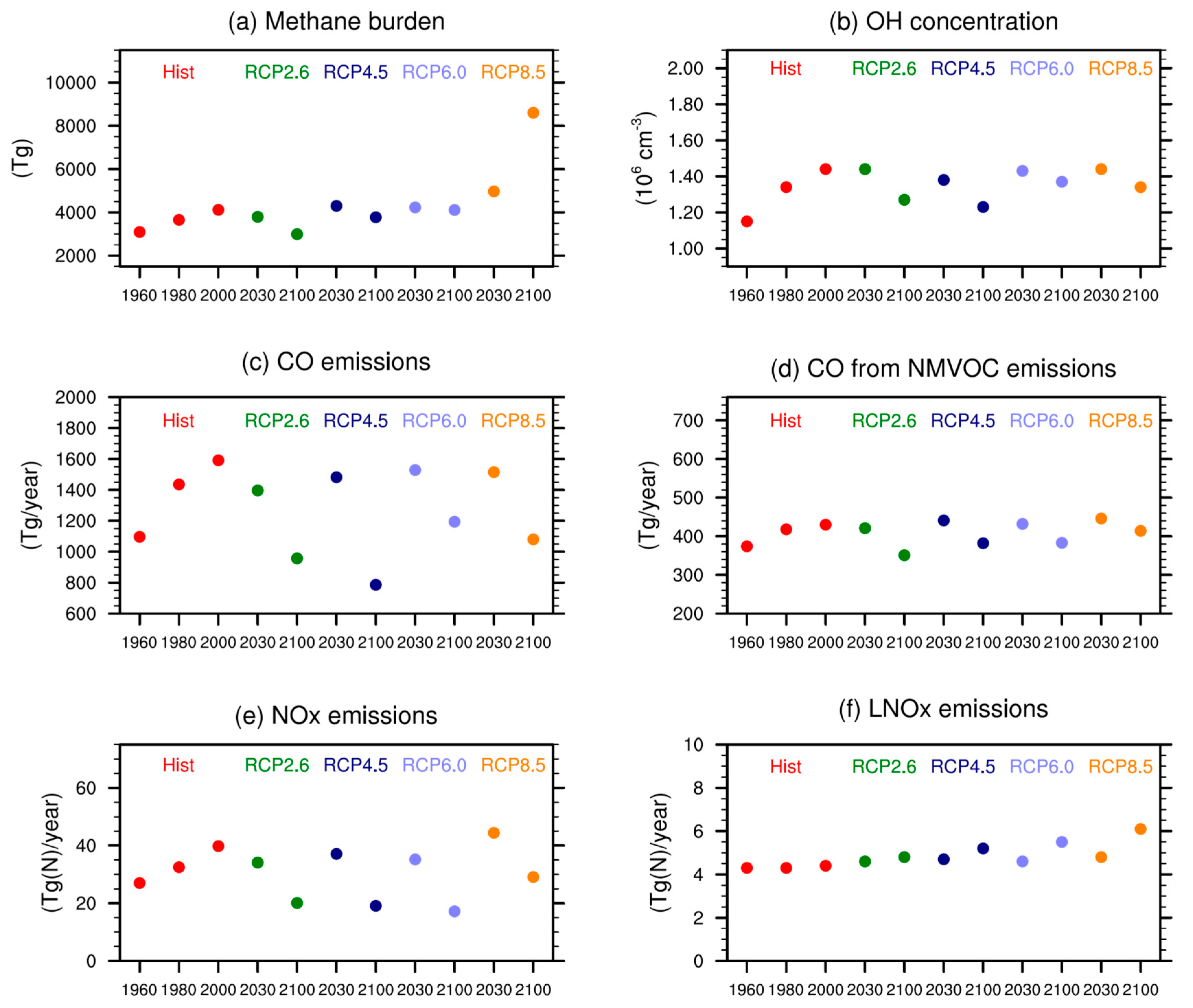
The ozone precursor emission scenarios prescribed for the RCPs assume that abundances of NOx, CO, and NMVOCs will decrease through the 21st century as nations take measures to reduce local air pollution. Methane, another key species for ozone, is prescribed as global mean surface mixing ratios. Between 1950 and 2000 methane concentrations increase from about 1150 ppb to 1750 ppb [55]. For the 21st century RCP 2.6, 4.5 and 6.0 assume methane concentrations to decrease to 1250 ppb, 1575 ppb and 1650 ppb, respectively. RCP 8.5 is distinctive in that substantial increases in methane concentrations are prescribed (from 1750 ppb to 3750 ppb between 2000 and 2100). Figure 1 shows ozone precursor emissions as well as methane burdens for different time slices and scenarios.
For all the simulations analyzed here, global mean surface mixing ratios of halocarbon ozone-depleting substances (ODSs) are prescribed following the A1 scenario from WMO (2011), which is based on observations until 2009 [64]. This scenario shows long-lived chlorine concentrations peaking around the year 2000, then steadily decreasing through the rest of the 21st century, following the implementation of the Montreal Protocol on Substances that Deplete the Ozone Layer and later amendments and adjustments.
Stratospheric aerosol properties are prescribed from the SAGE_4λ dataset [65,66]. The REF-C1 simulation uses transient aerosol properties, while the RCP simulations use the same aerosol properties each year (year 2000) since it is impossible to predict future volcanic eruptions. The year 2000 was a volcanically quiescent time, so the RCP simulations all assume no significant eruptions.
3.3. Tropospheric Ozone Chemistry
Ozone is produced and destroyed in the atmosphere via catalytic reaction cycles. Owing to the complex nature of these cycles and their interactions with one another in the troposphere, it is useful to highlight the fundamental reaction cycles here.
Ozone is produced in the troposphere following oxidation of CO (R1) or VOCs (Volatile Organic Compound, see (R2)):
CO + OH → CO2 + H
H + O2 + M → HO2 + M
HO2 + NO → NO2 + OH
NO2 + hν → NO + O
O + O2 + M → O3 + M
∑ CO + 2O2 → CO2 + O3
H + O2 + M → HO2 + M
HO2 + NO → NO2 + OH
NO2 + hν → NO + O
O + O2 + M → O3 + M
∑ CO + 2O2 → CO2 + O3
Here M is a third body (such as N2 or O2) that is needed to carry away excess energy for the reaction to occur. (R1) is the rate-limiting step and determines the overall rate of the reaction. Other reaction cycles producing NO2 occur following the oxidation of VOCs such as methane, formaldehyde, and isoprene, which can be generalized as:
RO2 + NO → NO2 + RO
Here R represents the organic part of the oxygen containing radicals RO2 and RO.
The most important initial source of OH radicals is the photolysis of O3:
O3 + hν → O(1D) + O2 (λ < 320 nm)
O(1D) + H2O → 2OH
∑ O3 + H2O + hν → O2 + 2OH
O(1D) + H2O → 2OH
∑ O3 + H2O + hν → O2 + 2OH
However, when the concentration of NOx is low (i.e., in clean air, remote from human activities), HO2 and RO2 instead react with ozone rather than NO, leading to overall ozone loss via (R4) and (R5):
CO + OH → CO2 + H
H + O2 + M → HO2 + M
HO2 + O3 → OH + 2O2
∑ CO + O3 → CO2 + O2
H + O2 + M → HO2 + M
HO2 + O3 → OH + 2O2
∑ CO + O3 → CO2 + O2
OH + O3 → HO2 + O2
HO2 + O3 → OH + 2O2
∑ 2O3 → 3O2
HO2 + O3 → OH + 2O2
∑ 2O3 → 3O2
In the tropics near the surface, which receive a lot of sunlight and have high humidity, (R3) can become the dominant ozone loss process.
4. Tropospheric Ozone Budget: Comparison of SOCOLv3 with Other Models
The tropospheric ozone budget includes chemical ozone production (P) and loss (L) (see Section 3.3), downward transport from the stratosphere (S), and dry deposition at the Earth’s surface (D). Before discussing trends in free tropospheric ozone (Section 5) we evaluate SOCOLv3’s tropospheric ozone budget through comparison with two previous tropospheric model evaluations, ACCENT [67] and ACCMIP [11]. Although this paper largely focuses on historical ozone trends, in this section we also show projected ozone burdens, in order to illustrate how ozone may evolve in future under different greenhouse gas and ozone precursor emission scenarios. While ACCENT and ACCMIP were based on year 2000 time slice simulations, the 1995–2005 average from the REF-C1 simulation is shown for SOCOLv3 (Table 3). The mean burden for SOCOLv3 is 413 Tg, and therefore about 80 Tg larger than the mean values reported for ACCENT and ACCMIP. Although there is a substantial spread among the simulated tropospheric ozone burdens (302 to 378 Tg), none of the ACCMIP models exceeds 400 Tg. A measurement-based estimate of 335 ± 10 Tg provided by Wild [35], although from pre-2000 data, supports the ACCENT and ACCMIP values.
SOCOLv3 not only overestimates the mean burden (B), but also ozone production and loss rates (Table 3). SOCOLv3’s high bias is difficult to explain. Young et al. [11] reported a high correlation between tropospheric ozone burden and total VOC emissions, with high VOC emissions leading to an enhanced ozone burden. The only NMVOC species directly emitted in SOCOL is isoprene (originating from biogenic emissions), and with 520 Tg year−1 the annual emissions are at the lower end of those used in the ACCMIP models. The main oxidizing agent in the troposphere is the hydroxyl radical (OH) and SOCOLv3’s mean tropospheric OH concentration (surface up to 200 hPa) for the year 2000 is 1.30 × 106 cm−3, compared to 1.11 × 106 cm−3 from the ACCMIP multi-model mean [68]. Enhanced methane (CH4) and VOC oxidation via OH would contribute to high tropospheric ozone production in NOx rich environments, in particular as SOCOL prescribes methane mixing ratios as lower boundary condition. As discussed below tropospheric ozone burdens in SOCOLv3 are indeed much more sensitive to NOx than in other models.
SOCOLv3 overestimates dry deposition compared to ACCENT and ACCMIP by approximately 50%. The difference can be explained by the simplified dry deposition scheme used in SOCOLv3, which applies constant deposition velocities over land and sea. (Dry deposition velocities used for ozone are 0.4 cm s−1 over land and 0.07 cm s−1 over sea). The dry deposition velocity for land is representative of vegetated surfaces, resulting in an overestimated dry deposition flux over snow-covered surfaces during winter. Initial sensitivity tests with a more sophisticated dry deposition scheme recently implemented into SOCOL reveal a dry deposition flux of around 1100 Tg(O3) year−1, much closer to the ACCENT and ACCMIP estimates. The stratospheric influx calculated from budget closure is 240 Tg year−1 for SOCOLv3, and therefore about half that of the other model ensemble mean estimates. Interestingly, the alternative estimate based on the origin tracers [20] results in a stratospheric influx of 491 Tg year−1, which is much closer to the ACCENT and ACCMIP values. SOCOLv3’s estimate of the ozone lifetime (τ) of 22.1 days agrees well with the values from ACCENT and ACCMIP. It should be noted, however, that the SOCOLv3 flux terms were not calculated in the same way as the ACCMIP and ACCENT ozone budgets, which might contribute to the differences presented here. For example, SOCOLv3’s dry deposition flux was not diagnosed during the simulation, but calculated afterwards from simulated ozone concentrations, and the ACCENT loss term does not include the reaction C5H8 + O3.
Figure 2 compares changes in tropospheric ozone burdens from SOCOLv3 with results from the ACCMIP models for the past as well as for several future projections (Table 5 and Figure 7 in [11]). As above, the ACCMIP results are based on time slice simulations, while for SOCOLv3 a 10-year average around the year of interest was calculated from transient simulations. The changes in ozone burdens were calculated with respect to the year 2000. Between 1980 and 2000 SOCOLv3’s tropospheric ozone burden increases by ~35 Tg (≈8% of the 2000 value), which is clearly larger than the ACCMIP average increase of 15 Tg (≈4%). In absolute terms, SOCOLv3 agrees reasonably well with the tropospheric ozone burden changes projected by the ACCMIP multi-model mean for 2030, but shows a more pronounced ozone decrease by 2100 for all scenarios except RCP 8.5. It should be noted that there is a large spread among the ACCMIP results for the 2030 time slices, with some models showing an increase compared to 2000 and others showing a decrease. For RCP 8.5 all models indicate increasing tropospheric ozone burdens in both 2030 and 2100. The relative changes for SOCOLv3 are −7% (−21%) in 2030 (2100) for RCP 2.6, 0% (−13%) for RCP 4.5, −2% (−15%) for RCP 6.0, and +10% (+14%) for RCP 8.5.
One potential reason for differences among models are differences in the ozone precursor emissions used. As described in Table 2, the boundary conditions for the SOCOLv3 simulations are based on observations for the hindcast REF-C1 simulation or follow the RCPs for the future projections. Therefore, they are supposed to be close to ACCMIP. However, differences in model parameterizations and complexity lead to some spread among the models. As expected, SOCOLv3’s tropospheric CH4 burdens (see Figure 1a in [11] for comparison) are very close to the ACCMIP multi-model mean since similar mixing ratios were prescribed as lower boundary conditions in most of the models. In contrast, tropospheric OH from SOCOLv3 is at the upper end of the ACCMIP model range for all periods and scenarios [67,68]. The direct CO emissions shown in Figure 1c are again at the upper end of ACCMIP. As oxidation of anthropogenic NMVOCs is not directly described in SOCOLv3 a certain fraction of NMVOCs is directly emitted as CO (see Section 3.1, Figure 1d). Constant isoprene emissions of 520 Tg year−1 are applied for all SOCOL simulations, which is in the lower range of biogenic VOC emissions in ACCMIP (Figure 1f in [13]). The annual NOx emissions used in SOCOL are again lower than the ACCMIP average. SOCOLv3’s lightning NOx emissions (LNOx) are between 4 and 6 Tg(N) year−1, depending on the scenario and time period, and therefore slightly below the ACCMIP average, but show a comparable increase in the future. Overall, it is unlikely that the differences in the tropospheric ozone burdens are related to the applied boundary conditions as they are within the same range as ACCMIP.
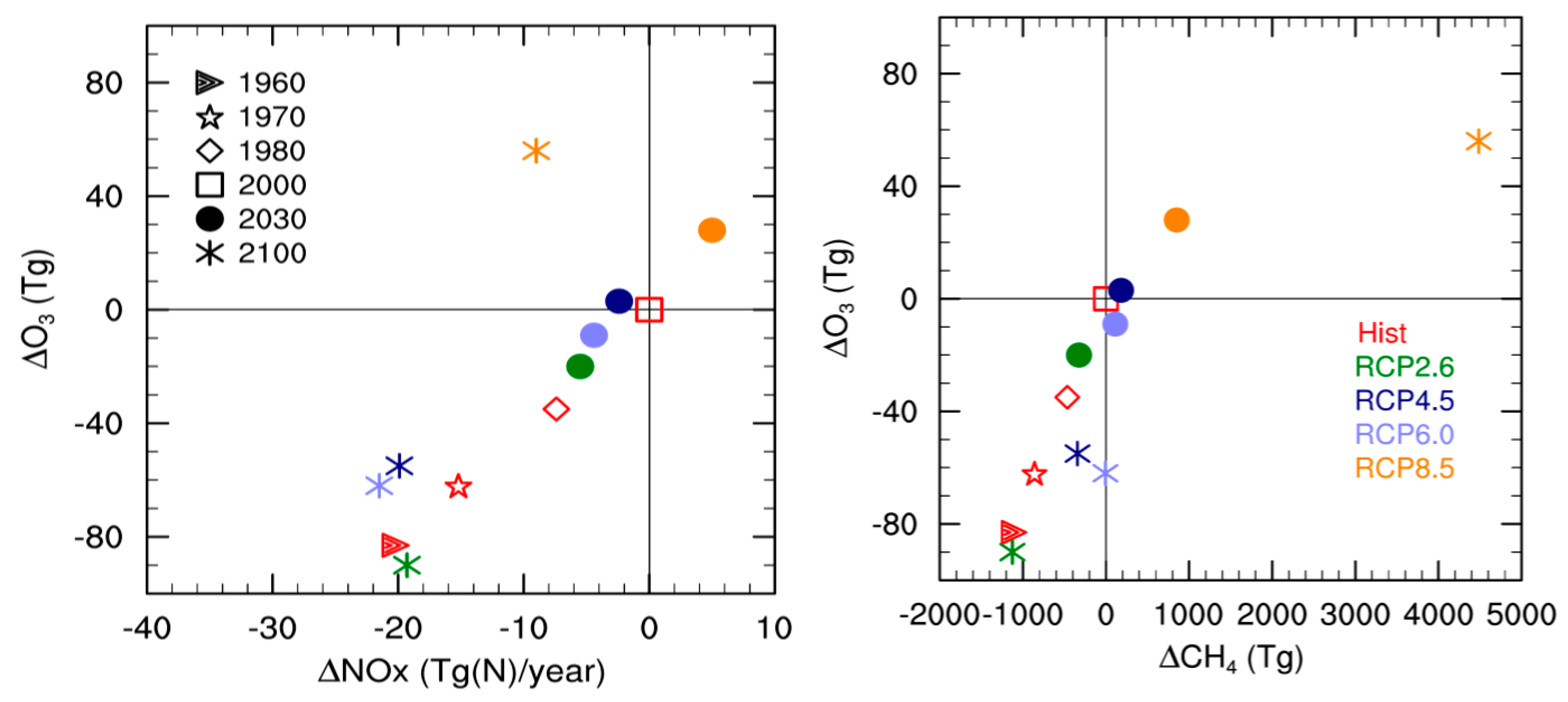
The relationship between tropospheric ozone burden, NOx emissions, and CH4 burdens has been widely discussed in previous studies e.g., [67]. Figure 3 shows the change in tropospheric ozone burden in SOCOLv3 as a function of changes in NOx emissions and CH4 burden for the different scenarios. Again, all changes are evaluated relative to the year 2000. For the past, SOCOLv3 shows an almost linear correlation between tropospheric ozone burden and NOx emissions. This linear relationship has also been found in previous studies e.g., [11,67]. However, on average SOCOLv3’s tropospheric ozone burden seems to be more sensitive to NOx emissions than the ACCMIP models (see Figure 13a in [11]). For RCP 2.6, 4.5, and 6.0, SOCOLv3 simulates a decrease in tropospheric ozone with decreasing NOx, but at a slightly lower rate than for the past. This is similar to what was found for the ACCMIP models. Previous studies explain this with an equatorward shift of ozone precursor emissions into a region with more efficient ozone production e.g., [69]. The clear correlation between NOx emissions and ozone burden no longer applies in RCP 8.5, which shows an ozone increase in 2100 despite lower NOx emissions (Figure 3, left). RCP 8.5 is characterized by an exceptionally large methane increase during the 21st century. The relationship between methane changes and tropospheric ozone burden is obviously not as linear as between NOx emissions and ozone, but is strongly influenced by the simulated burden of other ozone precursors [35]. The overall pattern for SOCOLv3 shown in Figure 3 is very similar to the ACCMIP findings, however SOCOLv3’s strong sensitivity to NOx leads to a more pronounced ozone decrease throughout the 21st century for RCPs 2.6, 4.5, and 6.0.
5. Comparison of SOCOL Simulations with Measurements
In this section, we restrict the comparison of results of SOCOLv3 to measurements from Alpine sites since (i) SOCOLv3’s tropospheric chemistry has already been evaluated using various satellite data sets [18]; and (ii) our analysis is focused on long-term ozone changes for which the most suitable measurements are from high altitude sites. Here we use measurements from Arosa (46.8° N, 9.7° E) and Jungfraujoch (46.55° N, 7.99° E). These sites belong to the same model grid box, which is centered at 46.04° N, 8.43° E. The mean altitude of the grid box is only 640 m, considerably lower than the real altitudes of Arosa (1775 m) and Jungfraujoch (3550 m).
In Figure 4 and Figure 5 measurements from Arosa are compared to the SOCOLv3 historical REF-C1 simulation. We extracted the data of the model level of 850 hPa, which corresponds to the physical altitude of Arosa (1775 m). The ozone annual cycle at Arosa differs between the model and the measurements (Figure 4), possibly because of the complex dynamics related to the mountainous topography of the Alpine area (termed “mountain venting” [70]), which are not resolved adequately in present global CCMs. We note that the measurements show somewhat larger increases in winter, similar to earlier analyses [29], while the model shows largest increases for the boreal summer period (July/August). (When using in Figure 4 SOCOL data of the grid box altitude (640 m) we found considerably lower ozone concentrations probably reflecting the effect of dry deposition in the model. However, the question remains whether a PBL comparable to open terrain exists in the alpine area due to the effect of mountain venting [70] making description of air pollutant concentration in the complex orography of the Alpine area challenging because global models cannot describe local features of alpine transport in any realistic way. As we are mainly interested in the long-term ozone changes we might ignore these problems assuming that these transport patterns might not have changed since the 1950s.
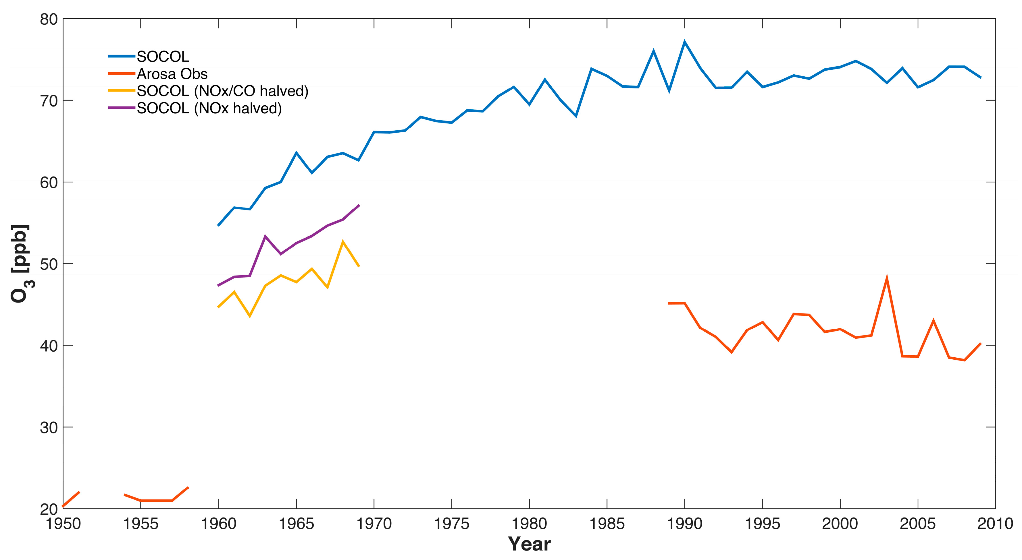
The ozone observations of Arosa show an increase in ozone from the 1950s to the early 1990s by a factor of around 2 similar to [29] in which the ozone increase from the 1950s to the years 1989–1991 was studied (see Figure 5). The increase in ozone in SOCOLv3 from the 1960 to 1990 is much smaller than in the observations, with an increase of around 30% (from 55 to 72 ppb). Even though the model simulation only starts in 1960, meaning there is no overlap with the 1950s measurements, it is obvious that the simulated ozone increase is considerably smaller than that observed. This under-estimation of long-term tropospheric ozone trends is characteristic of CCMs [15] (note that our analysis is not comparable with [15] in quantitative terms since we make no attempt to use the same polynomial fitting technique). The sensitivity tests for the 1960s with reduced emissions of anthropogenic ozone precursor emissions show only moderate decreases in simulated ozone concentrations, namely from 55 ppb to 47 ppb when reducing NOx by a factor 2 with unchanged CO and to 45 ppb when halving both NOx and CO simultaneously (see Figure 5). Neither measurements nor model show clear systematic changes since the early 1990s (a decrease might be expected because of decreasing ozone precursors of European countries as well as of North America, which will be further studied in [20]).
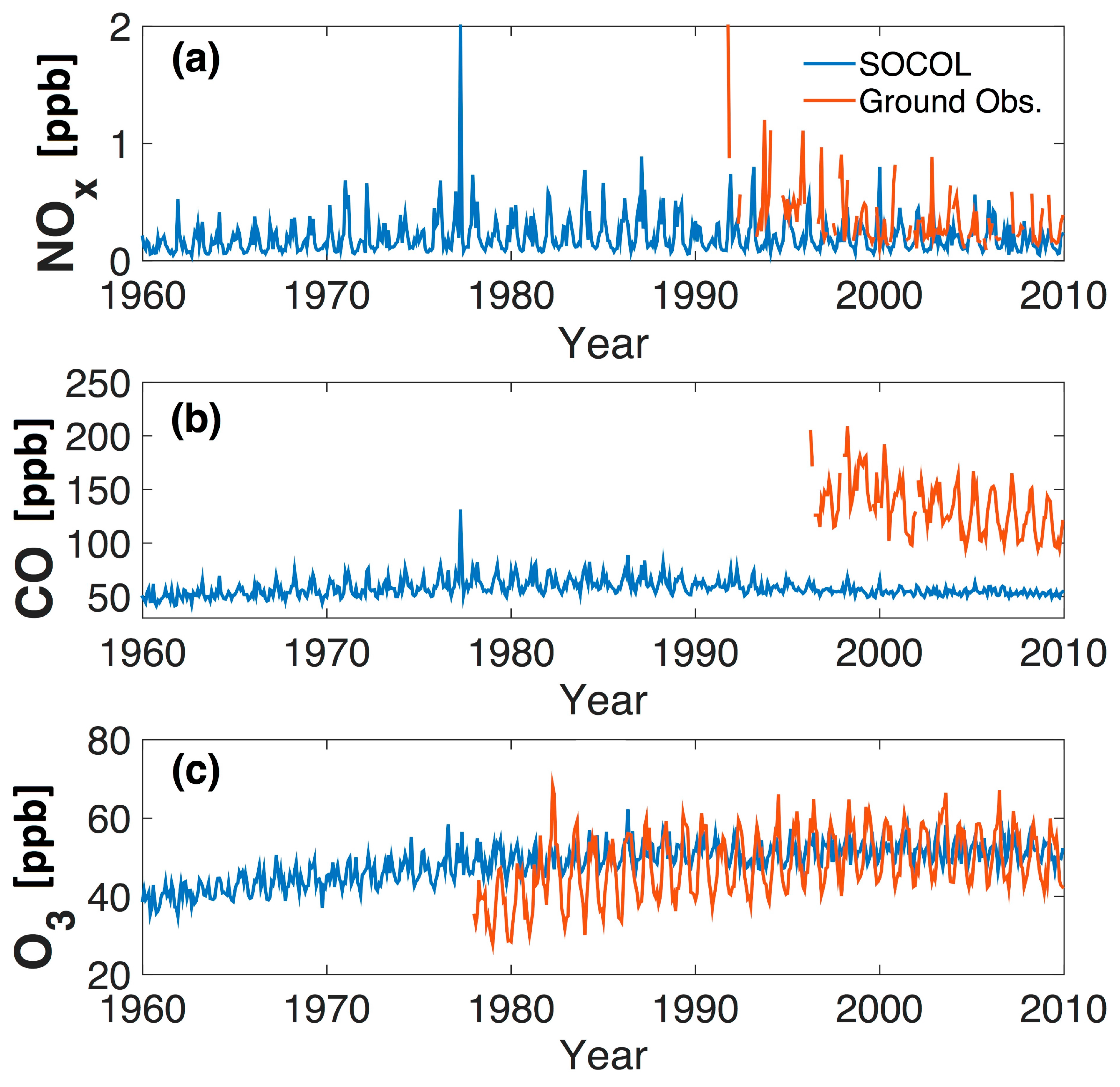
For Jungfraujoch, model data from the 700 hPa level are used corresponding to the physical altitude. The data should generally lie well within the model’s free troposphere (i.e., above the PBL). This corresponds well with the observations at Jungfraujoch, where the air sampled is only occasionally affected by the PBL [31]. Figure 6 shows the time series of several key trace gases at Jungfraujoch (CO and NOx) and an average high altitude Alpine data set for ozone constructed as described in [33] using observations from Zugspitze for the period 1978–1989 and a mean of Zugspitze, Jungfraujoch, and Sonnblick for the period 1990–2009. SOCOLv3 as well O3 measurements show approximately constant values since the turn of the century simulations being larger by around 20 ppb. However, the high alpine ozone series shows a much larger increase in the first decade (1980s) than SOCOLv3, in qualitative agreement with the long-term ozone evolution at Arosa (see Figure 5). NOx simulation and measurements compare from the middle of the 1990s onwards relatively well with the NOx measurements, showing fairly similar concentrations and decreasing NOx levels (a rough calculation of annual mean values shows a larger decrease in observations (−0.026 ppb/year) than in SOCOL simulations (0.005 ppb/year)).
SOCOLv3 underestimates CO concentrations at Jungfraujoch considerably (Figure 6) and does not show the same magnitude of downward trend (−0.24 ppb/year) as seen in the observations (−3.08 ppb/year). Rather, the simulated CO at Jungfraujoch (Figure 6) is remarkably constant over the 1960–2010 period. The fact that modeled CO mixing ratios at Jungfraujoch are much lower than measured could suggest that CO is oxidized much faster in the model than in reality. Indeed, simulated global mean annual OH concentrations range between 1.2–1.4 × 10⁻⁶ cm−3 (see Figure 1), and are therefore considerably higher than in most ACCMIP models (see Section 3), which is also reflected by rather short methane lifetimes of around 7 years in SOCOL compared to 9.7 year on average for the ACCMIP models [71]. Excessively high OH concentrations might be connected to high ozone production rates. (The high OH concentrations in SOCOL is the subject of ongoing studies).
6. Discussion and Conclusions
Ozone is the third most important greenhouse gas and its contribution to radiative forcing since pre-industrial times (1750) from changes in anthropogenic ozone precursor emissions has been calculated to be 410 m W m−2 (±17%, one standard deviation) [14]. This value was determined from a number of global tropospheric chemistry-climate models. In contrast to other greenhouse gases, pre-industrial ozone concentrations cannot be determined from archives such ice cores because ozone is a reactive gas and is not preserved in ice cores.
Validation of numerical simulations using measurements is important for a multitude of reasons. For present day conditions, tropospheric ozonesonde climatologies and measurements from many other reliable instrumental records including global records from several satellite instruments see e.g., [18] are available for comparison. It is difficult to assess whether model validation for present-day conditions is sufficient to test the reliability of simulations of a troposphere with strongly different composition. Validation using historical ozone observations is thus essential, but challenging given the dearth of reliable measurements. What measurements are available should be accurately assessed for quality and reliability, a task for which close cooperation between modeling and measurement experts is recommended. Ozone concentrations calculated from Schönbein papers should only be considered as semi-quantitative and should not be used for comparison with numerical simulations for validation of ozone values of the pre-industrial troposphere.
Only very few long-term surface ozone measurement series exist, and they are almost exclusively from northern mid-latitude sites. Even fewer have been judged useful in terms of providing representative measurements for evaluating long-term changes in tropospheric ozone. The only ozone measurements going back to the 1950s are from Europe and they can be considered reliable only as long as the interference from sulfur dioxide is small, which is true for the rural sites where these observations were made.
Our evaluation of the SOCOLv3 CCM with surface ozone measurements from the Arosa and Jungfraujoch Swiss Alpine sites confirm the main findings of [15], namely that current CCMs simulate smaller ozone increases than observed at northern mid-latitudes. For further confirmation our results should be compared with other model simulations performed within the CCMI activity, which have the advantage of using the same boundary conditions. It also might be useful to perform model simulations extending back to the 1950s, when surface ozone measurements are available, to allow overlap between simulations and the early surface ozone measurements.
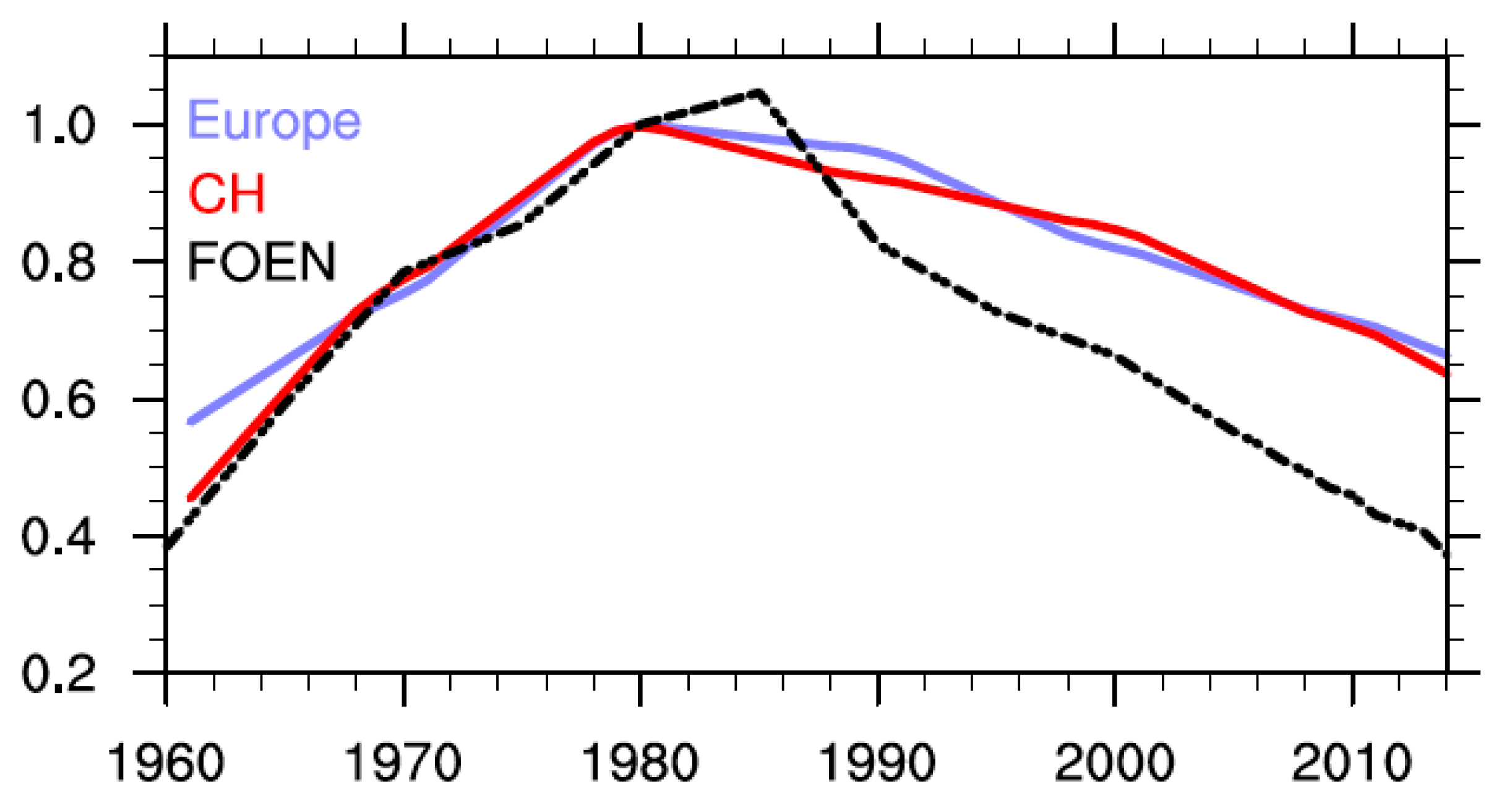
From a chemical perspective, this discrepancy might be attributable to problems in the emission data set used, however, changes in dynamical and transport processes are important for ozone changes over Europe as well [20]. Emissions of ozone precursors are a key factor for accurately simulating long-term ozone changes. Figure 7 compares the temporal development of annual NOx emissions used in the REF-C1 simulation from Europe and Switzerland as well as national NOx emissions as reported by FOEN (Swiss Federal Office for Environment), the Swiss Federal Office for Environment [72]. All values are shown relative to the year 1980. In contrast to the FOEN emissions, which show a maximum in 1985, the emission data set prescribed for the REF-C1 simulation peaks in 1980. While the increase in Swiss NOx emissions in the model is similar to the trend reported by FOEN, the increase is less pronounced for the greater European region. It seems surprising that NOx emission increases from the 1960s would be much smaller for Europe than for Switzerland since the strong economic growth that started in the 1950s continued in all industrialized countries for several decades. Differences in NOx emissions are evident after 1985 as the data set used in the REF-C1 simulation clearly underestimates the decline in NOx emissions as reported by FOEN. The MAC City emission inventory (Figure 12c in [15]) used as input in the CCMI simulations shows a rather small NOx increase for 15°–70° N for the 1960–1985 period. In a recent study [73] significant differences were found between the long-term evolution of NOx and CO emissions derived from fossil fuel usage and long-term monitoring measurements from cities in the USA and Europe (Paris (France) and London (UK)) and the MAC City bottom-up emission inventory. This study illustrates the uncertainties related to anthropogenic emissions inventories, particularly regarding the long-term evolution of these emissions.
We might speculate that emission estimates of ozone precursors for the 1960s are too high, resulting in a smaller-than-observed simulated increase in ozone. In this regard, it is important to note that there are almost no historical emission factors available [74]. These emission factors are essential to calculating bottom-up emissions estimates and thus may play a role in potential biases in the underlying emissions inventories used here. This hypothesis might further be supported by the fact that a range of CCMs show similarly small increases in tropospheric ozone over the past five decades.
The problem described here does not necessarily mean that the pre-industrial emissions as used by the IPCC are erroneous. The same emissions are used in IPCC and CCMI (Table 7 in [12]): Global NOx emissions show a very large increase from 1850 to 1930 (approximately a factor of ten) followed by a further steep increase that started around 1940. The large increase in NOx emissions prior to World War II might be viewed as somewhat unexpected since large NOx emissions occur generally only from high temperature combustion technologies (implying the use of gasoline or oil, e.g., as used in road traffic engines). The use of coal, however, was rather common before World War II and thus NOx emissions are likely to have been comparatively small. We therefore might speculate that if the large increase in ozone precursor species occurred later than as described in current emission inventories, simulated ozone concentrations for the 1960s would be lower and result in a larger increase to the 1990s.
Acknowledgments
To stress the key importance of reliable ozone measurements we like to thank Hans-Eckhart Scheel (measurements at Zugspitze) and Jürg Thudium (measurements at Arosa). Fiona Tummon is supported by SNSF post-doctoral grant (No. 20FI21_138017). For results of numerical simulations see: Chemistry-Climate Model Initiative (CCMI-1) Project Database, NCAS British Atmospheric Data Centre, available at: http://catalogue.ceda.ac.uk/uuid/1005d2c25d14483aa66a5f4a7f50fcf0 (20 October 2016), 2015. We thank for the careful reviews and the help of the assistant editor.
Author Contributions
The article is the result of a team work: Johannes Staehelin particularly contributed by the review of the ozone measurements, Fiona Tummon made the comparison of numerical simulations and observations of alpine sites, Laura Revell provided the presented numerical simulations, Andrea Stenke was responsible for the analysis of the ozone budget and Thomas Peter supported the work by his important contribution to the design of the study and critical review.
Conflicts of Interest
The authors declare no conflict of interest.
References
- Grosjean, D. Ambient PAN and PPN in southern California from 1960 to the SCOS97-NASTRO. Atmos. Environ. 2003, 37 (Suppl. 2), S221–S238. [Google Scholar] [CrossRef]
- Haagen-Smit, A. Chemistry and Physiology of Los Angeles Angeles Smog. Ind. Eng. Chem. Res. 1952, 44, 1342–1346. [Google Scholar] [CrossRef]
- Martien, P.T.; Harley, R.A. Adjoint sensitivity analysis for a three dimensional photochemical model: Application to Southern California. Environ. Sci. Technol. 2006, 40, 4200–4210. [Google Scholar] [CrossRef] [PubMed]
- South Coast Air Quality Management District. Available online: http://www.aqmd.gov/home/library/air-quality-data-studies/historic-ozone-air-quality-trends (accessed on 21 August 2017).
- World Meteorological Organization: Scientific Assessment of Ozone Depletion: 2014; Report No. 55; WMO Global Ozone Research and Monitoring Project: Geneva, Switzerland, 2014.
- Stocker, T.F.; Qin, D. Climate Change 2013: The Physical Science Basis. Contribution of Working Group I to the Fifth Assessment Report of the Intergovernmental Panel on Climate Change; Cambridge University Press: Cambridge, UK; New York, NY, USA, 2013. [Google Scholar]
- Task Force on Hemispheric Transport of air pollution (HTAP). Available online: www.htap.org (accessed on 21 August 2017).
- Cooper, O.R.; Parrish, D.D.; Stohl, A.; Trainer, M.; Nédélec, P.; Thouret, V.; Cammas, J.P.; Oltmans, S.J.; Johnson, B.J.; Tarasick, D.; et al. Increasing springtime ozone mixing ratio in the free troposphere over western North America. Nature 2010, 463, 344–348. [Google Scholar] [CrossRef] [PubMed]
- Fiore, A.M.; Dentener, F.J.; Wild, O.; Cuvelier, C.; Schultz, M.G.; Hess, P.; Textor, C.; Schulz, M.; Doherty, R.M.; Horowitz, W.; et al. Multimodel estimates of intercontinental source-receptor relationships for ozone pollution. J. Geophys. Res. 2009, 114, D04301. [Google Scholar] [CrossRef]
- Ordonez, C.; Brunner, D.; Staehelin, J.; Hadjinicolaou, P.; Pyle, J.A.; Jonas, M.; Wernli, H.; Prevot, A.S.H. Strong influence of lowermost stratospheric ozone on lower tropospheric background ozone changes over Europe. Geophys. Res. Lett. 2007, 34. [Google Scholar] [CrossRef]
- Young, P.J.; Archibald, A.T.; Bowman, K.W.; Lamarque, J.-F.; Naik, V.; Stevenson, D.S.; Tilmes, S.; Voulgarakis, A.; Wild, O.; Bergmann, D.; et al. Pre-industrial to end 21st century projections of tropospheric ozone from the Atmospheric Chemistry and Climate Model Intercomparison Project (ACCMIP). Atmos. Chem. Phys. 2013, 13, 2063–2090. [Google Scholar] [CrossRef] [Green Version]
- Lamarque, J.F.; Bond, T.C.; Eyring, V.; Granier, C.; Heil, A.; Klimont, Z.; Lee, D.; Liousse, C.; Mieville, A.; Owen, B.; et al. Historical (1850–2000) gridded anthropogenic and biomass burning emissions of reactive gases and aerosols: Methodology and application. Atmos. Chem. Phys. 2010, 10, 7017–7039. [Google Scholar] [CrossRef] [Green Version]
- Lamarque, J.-F.; Shindell, D.T.; Josse, B.; Young, P.J.; Cionni, I.; Eyring, V.; Bergmann, D.; Cameron-Smith, P.; Collins, W.J.; Doherty, R.; et al. The Atmospheric Chemistry and Climate Model Intercomparison Project (ACCMIP): Overview and description of models, simulations and climate diagnostics. Geosci. Model Dev. 2013, 6, 179–206. [Google Scholar] [CrossRef] [Green Version]
- Stevenson, D.S.; Young, P.J.; Naik, V.; Lamarque, J.-F.; Shindell, D.T.; Voulgarakis, A.; Skeie, R.B.; Dalsoren, S.B.; Myhre, G.; Berntsen, T.K.; et al. Tropospheric ozone changes, radiative forcing and attribution to emissions in the Atmospheric Chemistry and Climate Model Intercomparison Project (ACCMIP). Atmos. Chem. Phys. 2013, 13, 3063–3085. [Google Scholar] [CrossRef] [Green Version]
- Parrish, D.D.; Lamarque, J.-F.; Naik, V.; Horowitz, L.; Shindell, D.T.; Staehelin, J.; Derwent, R.; Cooper, O.R.; Tanimoto, H.; Volz-Thomas, A.; et al. Long-term changes in lower tropospheric baseline ozone concentrations: Comparing chemistry-climate models and observations at northern mid-latitudes. J. Geophys. Res. 2014, 119, 5719–5736. [Google Scholar] [CrossRef]
- Parrish, D.D.; Law, K.S.; Staehelin, J.; Derwent, R.; Cooper, O.R.; Tanimoto, H.; Volz Thomas, A.; Gilge, S.; Scheel, H.-E.; Steinbacher, M.; et al. Long-term changes in lower tropospheric baseline ozone concentrations at northern mid-latitudes. Atmos. Chem. Phys. 2012, 12, 11485–11504. [Google Scholar] [CrossRef] [Green Version]
- Parrish, D.D.; Law, K.S.; Staehelin, J.; Derwent, R.; Cooper, O.R.; Tanimoto, H.; Volz Thomas, A.; Gilge, S.; Scheel, H.-E.; Steinbacher, M.; et al. Lower tropospheric ozone at northern mid-latitudes: Changing seasonal cycle. Geophys. Res. Lett. 2013, 40, 1631–1636. [Google Scholar] [CrossRef]
- Revell, L.E.; Tummon, F.; Stenke, A.; Sukhodolov, T.; Coulon, A.; Rozanov, E.; Garny, H.; Grewe, V.; Peter, T. Drivers of the tropospheric ozone budget throughout the 21st century under the medium-high climate scenario RCP 6.0. Atmos. Chem. Phys. 2015, 15, 5887–5902. [Google Scholar] [CrossRef] [Green Version]
- Stenke, A.; Schraner, M.; Rozanov, E.; Egorova, T.; Luo, B.; Peter, T. The SOCOL version 3.0 chemistry-climate model: Description, evaluation, and implications from an advanced transport algorithm. Geosci. Model Dev. 2013, 6, 1407–1427. [Google Scholar] [CrossRef]
- Tummon, F.; Revell, L.; Stenke, A.; Staehelin, J.; Peter, T. Diagnosing Changes in European Free Tropospheric Ozone Over the Past 35 Years. 2017; in preparation. [Google Scholar]
- TOAR. Available online: http://www.igacproject.org/activities/TOAR (accessed on 21 August 2017).
- Rubin, M.B. The history of ozone. The Schönbein period, 1839–1868. Bull. Hist. Chem. 2001, 26, 40–56. [Google Scholar]
- Wolf, R. Ozongehalt der Luft und seinen Zusammenhang mit der Mortalität. In Vorträge in der Bernischen Naturforschenden Gesellschaft, Bern; Verlag Huber & Comp.: Bern, Switzerland, 1855. [Google Scholar]
- Fox, C.B. Ozone and Antozone; Churchill Publisher: London, UK, 1873. [Google Scholar]
- Kley, D.; Volz, A.; Mülheim, F. Ozone measurements in historic perspective. In Tropospheric Ozone; Isaksen, I.S.A., Ed.; D. Reidel: Kufstein, Österreich, 1988; pp. 63–73. [Google Scholar]
- Pavelin, E.G.; Johnson, C.E.; Rughooputh, S.; Toumi, R. Evaluation of pre-industrial surface ozone measurements made using Schönbein’s method. Atmos. Environ. 1999, 33, 919–929. [Google Scholar] [CrossRef]
- Volz, A.; Kley, D. Evaluation of the Montsouris series of ozone measurements made in the nineteenth century. Nature 1988, 332, 240–242. [Google Scholar] [CrossRef]
- Staehelin, J.; Brönnimann, S.; Peter, T.; Stübi, R.; Viatte, P.; Tummon, F. The value of Swiss long-term ozone observations for international atmospheric research. In From Weather Observations to Atmospheric and Climate Sciences in Switzerland—Celebrating 100 Years of the Swiss Society for Meteorology; Willemse, S., Furger, M., Eds.; vdf Hochschulverlag AG: Zürich, Switzerland, 2016; pp. 325–349. [Google Scholar]
- Staehelin, J.; Thudium, J.; Bühler, R.; Volz-Thomas, A.; Graber, W. Surface ozone trends at Arosa (Switzerland). Atmos. Environ. 1994, 28, 75–87. [Google Scholar] [CrossRef]
- Derwent, R.G.; Simmonds, P.G.; Manning, A.J.; Spain, T.G. Trends over a 20-year period from 1987 to 2007 in surface ozone at the atmospheric research station, Mace Head, Ireland. Atmos. Environ. 2007, 41, 9091–9098. [Google Scholar] [CrossRef]
- Cui, J.; Pandey Deolal, S.; Sprenger, M.; Henne, S.; Staehelin, J.; Steinbacher, M.; Nedelec, P. Free tropospheric ozone changes over Europe as observed at Jungfraujoch (1990–2008): An analysis based on backward trajectories. J. Geophys. Res. 2011, 116, D10304. [Google Scholar] [CrossRef]
- Atmospheric Ozone 1985, Assessment of Our Understanding of the Processes Controlling Its Present Distribution and Change; Global Ozone Research and Monitoring Project 16; World Meteorological Organization (WMO): Geneva, Switzerland, 1985; Volume II, pp. 410–411.
- Logan, J.A.; Staehelin, J.; Megretskaia, I.A.; Cammas, J.-P.; Thouret, V.; Claude, H.; De Backer, H.; Steinbacher, M.; Scheel, H.-E.; Stübi, R.; et al. Changes in ozone over Europe: Analysis of ozone measurements from sondes, regular aircraft (MOZAIC) and alpine surface sites. J. Geophys. Res. 2012, 117, D09301. [Google Scholar] [CrossRef]
- Smit, H. The Panel for Assessment of Standard Operating Procedures for Ozonsondes (ASOPOS), 2011: Quality Assurance and Quality Control for Ozonesonde Measurements in GAW; GAW Report 201; World Meteorological Organization: Geneva, Switzerland, 2011. [Google Scholar]
- Wild, O. Modelling the global tropospheric ozone budget: Exploring the variability in current models. Atmos. Chem. Phys. 2007, 7, 2643–2660. [Google Scholar] [CrossRef]
- Schnadt Poberaj, C.; Staehelin, J.; Brunner, D.; Thouret, V.; Mohnen, V. A UT/LS ozone climatology of the nineteen seventies deduced from the GASP aircraft measurement program. Atmos. Chem. Phys. 2007, 7, 5917–5936. [Google Scholar] [CrossRef]
- Dias-Lalcaca, P.; Brunner, D.; Imfeld, W.; Moser, W.; Staehelin, J. An automated system for the measurement of nitrogen oxides and ozone concentrations from a passenger aircraft: Instrumentation and first results of the project NOXAR. Environ. Sci. Technol. 1998, 32, 3228–3236. [Google Scholar] [CrossRef]
- Brunner, D.; Staehelin, J.; Jeker, D.; Wernli, H.; Schumannm, U. Nitrogen oxides and ozone in the tropopause region of the Northern Hemisphere: Measurements from commercial aircraft in 1995/96 and 1997. J. Geophys. Res. 2001, 106, 27673–27699. [Google Scholar] [CrossRef]
- Thouret, V.; Cammas, J.-P.; Sauvage, B.; Athier, B.; Zbinden, R.M.; Nédélec, P.; Simmon, P.; Karcher, F. Tropopause referenced ozone climatology and inter-annual variability (1994–2003) from MOZAIC programme. Atmos. Chem. Phys. 2006, 6, 1033–1051. [Google Scholar] [CrossRef]
- Brenninkmeijer, C.A.M.; Crutzen, P.; Boumard, F.; Dauer, T.; Dix, B.; Ebinghaus, R.; Filippi, D.; Fischer, H.; Franke, H.; Frie, B.; et al. Civil Aircraft for the regular investigation of the atmosphere based on an instrumented container: The new CARIBIC system. Atmos. Chem. Phys. 2007, 7, 4953–4976. [Google Scholar] [CrossRef] [Green Version]
- IAGOS Data Portal. Available online: http://iagos.sedoo.fr/ (accessed on 21 August 2017).
- Schnadt Poberaj, C.; Staehelin, J.; Brunner, D.; Thouret, V.; De Backer, H.; Stübi, R. Long-term changes in UT/LS ozone between the late 1970s and the 1990s deduced from the GASP and MOZAIC aircraft programs and from ozonesonde. Atmos. Chem. Phys. 2009, 9, 5343–5369. [Google Scholar] [CrossRef]
- Staufer, J.; Staehelin, J.; Stübi, R.; Peter, T.; Tummon, F.; Thouret, V. Trajectory matching of ozonesondes and MOZAIC measurements in the UTLS, Part II: Application to the global ozonesonde network. Atmos. Meas. Technol. 2014, 7, 241–266. [Google Scholar] [CrossRef] [Green Version]
- Van der A, R.J.; Eskes, H.J.; Boersma, K.F.; van Noije, T.P.C.; Van Roozendael, M.; De Smedt, I.; Peters, D.H.M.U.; Meijer, E.W. Trends, seasonal variability and dominant NOx source derived for a ten year record of NO2 measured from space. J. Geophys. Res. 2008, 113, D04302. [Google Scholar] [CrossRef]
- Oltmans, S.J.; Lefohn, A.S.; Harris, J.M.; Galbally, J.; Scheel, H.S.; Bodecker, G.; Brunke, E.; Claude, H.; Tarasick, D.; Johnson, B.J.; et al. Long-term changes in tropospheric ozone. Atmos. Environ. 2006, 40, 3156–3173. [Google Scholar] [CrossRef]
- Cooper, O.R.; Parrish, D.D.; Ziemke, J.; Balashov, N.V.; Cupeiro, M.; Galbally, I.E.; Gilge, S.; Horowitz, L.; Jensen, N.R.; Lamarque, J.F.; et al. Global distribution and trends of tropospheric ozone: An observation based review. Elementa 2014, 2, 000029. [Google Scholar] [CrossRef]
- Roeckner, E.; Bäuml, G.; Bonaventura, L.; Brokopf, R.; Esch, M.; Giorgetta, M.; Hagemann, S.; Kirchner, I.; Kornblueh, L.; Manzini, E.; et al. The Atmospheric General Circulation Model ECHAM 5. Part I: Model Description; Report No. 349; Max-Planck-Institut für Meteorologie: Hamburg, Germany, 2003; Available online: http://pubman.mpdl.mpg.de/pubman/faces/viewItemFullPage.jsp?itemId=escidoc:995269:2 (accessed on 4 March 2017).
- Egorova, T.A.; Rozanov, E.V.; Zubov, V.A.; Karol, I.L. Model for investigating ozone trends (MEZON). Izv. Atmos. Ocean. Phys. 2003, 39, 277–292. [Google Scholar]
- Chang, J.S.; Brost, R.A.; Isaksen, I.S.A.; Madronich, S.; Middleton, P.; Stockwell, W.R.; Walcek, C.J. A three dimensional Eulerian acid deposition model: Physical concepts and formulation. J. Geophys. Res. 1987, 92, 14681–14700. [Google Scholar] [CrossRef]
- Poeschl, U.; von Kuhlmann, R.; Poisson, N.; Crutzen, P.J. Development and intercomparison of condensed isoprene oxidation mechanisms for global atmospheric modeling. J. Atmos. Chem. 2000, 37, 29–52. [Google Scholar] [CrossRef]
- Ehhalt, D.; Prather, M.; Dentener, F.; Derwent, R.; Dlugokencky, E.; Holland, E.; Isaksen, I.; Katima, J.; Kirchhoff, V.; Matson, P.; et al. Atmospheric chemistry and greenhouse gases. In Climate Change 2001: The Scientific Basis. Contribution of Working Group I to the Third Assessment Report of the Intergovernmental Panel on Climate Change; Houghton, J.T., Ding, Y., Griggs, D.J., Noguer, M., van der Linden, P.J., Dai, X., Maskell, K., Johnson, C.A., Eds.; Cambridge University Press: Cambridge, UK; New York, NY, USA, 2001. [Google Scholar]
- Price, C.; Rind, D. A simple lightning parameterization for calculating global lightning distributions. J. Geophys. Res. 1992, 97, 9919–9933. [Google Scholar] [CrossRef]
- Grewe, V. The origin of ozone. Atmos. Chem. Phys. 2006, 6, 1495–1511. [Google Scholar] [CrossRef]
- Garny, H.; Grewe, V.; Dameris, M.; Bodeker, G.E.; Stenke, A. Attribution of ozone changes to dynamical and chemical processes in CCMs and CTMs. Geosci. Model Dev. 2011, 4, 271–286. [Google Scholar] [CrossRef] [Green Version]
- Meinshausen, M.; Smith, S.J.; Calvin, K.; Daniel, J.S.; Kainuma, M.L.T.; Lamarque, J.-F.; Matsumoto, K.; Montzka, S.A.; Raper, S.C.B.; Riahi, K.; et al. The RCP greenhouse gas concentrations and their extensions from 1765 to 2300. Clim. Chang. 2011, 109, 213–241. [Google Scholar] [CrossRef]
- Riahi, K.; Rao, S.; Krey, V.; Cho, C.; Chirkov, V.; Fischer, G.; Kindermann, G.; Nakicenovic, N.; Rafaj, P. RCP 8.5—A scenario of comparatively high greenhouse gas emissions. Clim. Chang. 2011, 109, 33–57. [Google Scholar] [CrossRef]
- Rayner, N.A.; Parker, D.E.; Horton, E.B.; Folland, C.K.; Alexander, L.V.; Rowell, D.P.; Kent, E.C.; Kaplan, A. Global analyses of sea surface temperature, sea ice, and night marine air temperature since the late nineteenth century. J. Geophys. Res. 2003, 108, 4407. [Google Scholar] [CrossRef]
- Van Vuuren, D.P.; Stehfest, E.; den Elzen, M.G.J.; Kram, T.; van Vliet, J.; Deetman, S.; Isaac, M.; Klein Goldewijk, K.; Hof, A.; Mendoza Beltram, A.; et al. RCP2.6: Exploring the possibility to keep global mean temperature increase below 2 °C. Clim. Chang. 2011, 109, 95–116. [Google Scholar] [CrossRef]
- Meehl, G.A.; Washington, W.M.; Arblaster, J.M.; Hu, A.; Teng, H.; Kay, J.E.; Gettelman, A.; Lawrence, D.M.; Sanderson, B.M.; Strand, W.G. Climate change projections in CESM1(CAM5) compared to CCSM4. J. Clim. 2013, 26, 6287–6308. [Google Scholar] [CrossRef]
- Thomson, A.M.; Calvin, K.V.; Smith, S.J.; Page Kyle, G.; Volke, A.; Patel, P.; Delgado-Arias, S.; Bond-Lamberty, B.; Wise, M.A.; Clarke, L.E.; et al. RCP 4.5: A pathway for stabilization of radiative forcing by 2100. Clim. Chang. 2011, 109, 77–94. [Google Scholar] [CrossRef]
- Masui, T.; Matsumoto, K.; Hijioka, Y.; Kinoshita, T.; Nozawa, T.; Ishiwatari, S.; Kato, E.; Shukla, P.R.; Yamagata, Y.; Kainuma, M. An emission pathway for stabilization at 6 Wm−2 radiative forcing. Clim. Chang. 2011, 109, 59–76. [Google Scholar] [CrossRef]
- Morgenstern, O.; Hegglin, M.I.; Rozanov, E.; O’Connor, F.M.; Abraham, N.L.; Akiyoshi, H.; Archibald, A.T.; Bekki, S.; Butchart, N.; Chipperfield, M.P.; et al. Review of the global models used within phase 1 of the Chemistry–Climate Model Initiative (CCMI). Geosci. Model Dev. 2017, 10, 639–671. [Google Scholar] [CrossRef]
- Van Vuuren, D.P.; Edmonds, J.; Kainuma, M.; Riahi, K.; Thomson, A.; Hibbard, K.; Hurtt, C.G.; Kram, T.; Krey, V.; Lamarque, J.-F.; et al. The representative concentration pathways: An overview. Clim. Chang. 2011, 109, 5–31. [Google Scholar] [CrossRef]
- Scientific Assessment of Ozone Depletion: 2010; Global Ozone Research and Monitoring Project—Report No. 52; World Meteorological Organization (WMO): Geneva, Switzerland, 2011.
- Arfeuille, F.; Luo, B.P.; Heckendorn, P.; Weisenstein, D.; Sheng, J.X.; Rozanov, E.; Schraner, M.; Brönnimann, S.; Thomason, L.W.; Peter, T. Modeling the stratospheric warming following the Mt. Pinatubo eruption: Uncertainties in aerosol extinctions. Atmos. Chem. Phys. 2013, 13, 11221–11234. [Google Scholar]
- Luo, B.P. Stratospheric Aerosol Data for Use in CCMI Models. 2013. Available online: ftp://iacftp.ethz.ch/pub_read/luo/ccmi/ (accessed on 23 August 2017).
- Stevenson, D.S.; Dentener, F.J.; Schultz, M.G.; Ellingsen, K.; van Noije, T.P.C.; Wild, O.; Zeng, G.; Amann, M.; Atherton, M.; Bell, N.; et al. Multimodel ensemble simulations of present-day and near-future tropospheric ozone. J. Geophys. Res. 2006, 111, D08301. [Google Scholar] [CrossRef]
- Naik, V.; Voulgarakis, A.; Fiore, A.M.; Horowitz, L.W.; Lamarque, J.-F.; Lin, M.; Prather, M.J.; Young, P.J.; Bergmann, D.; Cameron-Smith, P.J.; et al. Preindustrial to present-day changes in tropospheric hydroxyl radical and methane lifetime from the Atmospheric Chemistry and Climate Model Intercomparison Project (ACCMIP). Atmos. Chem. Phys. 2013, 13, 5277–5298. [Google Scholar] [CrossRef] [Green Version]
- Wild, O.; Palmer, P.I. How sensitive is tropospheric oxidation to anthropogenic emissions? Geophys. Res. Lett. 2008, 35, L22802. [Google Scholar] [CrossRef]
- Henne, S.; Dommen, D.; Neininger, B.; Reimann, S.; Staehelin, J.; Prévôt, A.S.H. Influence of mountain venting in the Alps on the ozone chemistry of the lower free troposphere and the European pollution export. J. Geophys. Res. 2005, 110, D22307. [Google Scholar] [CrossRef]
- Voulgarakis, A.; Naik, V.; Lamarque, J.-F.; Shindell, D.T.; Young, P.J.; Prather, M.J.; Wild, O.; Field, R.D.; Bergmann, D.; Cameron-Smith, P.; et al. Analysis of present day and future OH and methane lifetime in the ACCMIP simulations. Atmos. Chem. Phys. 2013, 13, 2563–2587. [Google Scholar] [CrossRef] [Green Version]
- Vom Menschen Verursachte Luftschadstoff-Emissionen in der Schweiz von 1900 bis 2010; Schriftenreihe Umwelt No. 255; Bundesamt für Umwelt, Wald und Landschaft (BUWAL/FOEN): Bern, Switzerland, 1995.
- Hassler, B.; McDonald, B.C.; Frost, G.J.; Borbon, A.; Carslaw, D.C.; Civerolo, K.; Granier, C.; Monks, P.S.; Monks, S.; Parrish, D.D.; et al. Analysis of long-term observation of NOx and CO in megacities and application to constraining emission inventories. Geophys. Res. Lett. 2016, 43, 9920–9930. [Google Scholar] [CrossRef]
- Van Aardenne, J.A.; Dentener, F.J.; Olivier, J.G.J.; Klein Goldewijk, C.G.M.; Lelieveld, J. A 1ox1o resolution data set of historical anthropogenic trace gas emissions for the period 1890–1990. Glob. Beogeochem. Cycles 2001, 15, 909–928. [Google Scholar] [CrossRef]
Figure 1.
Emissions used for the SOCOLv3 (Solar Climate Ozone Links version 3) simulations carried out for this study, as well as SOCOLv3 tropospheric burdens of important species. (a) tropospheric methane burden; (b) tropospheric mean OH concentrations; (c) annual total CO emissions; (d) CO from NMVOC (Non Methane Volatile Organic Compound) oxidation; (e) total NOx emissions; and (f) lightning NOx emissions calculated online based on the cloud top height.

Figure 2.
Change in the tropospheric ozone burden (Tg) for the different scenarios, relative to year 2000 values. The filled circles show SOCOLv3 results, while the open diamonds show the ACCMIP (Atmospheric Chemistry and Climate Model Intercomparison Project) multi model mean. The minimum-maximum range for ACCMIP is indicated by the vertical lines. For clarity the data points showing SOCOL and ACCMIP data have been slightly offset with respect to the time axis.
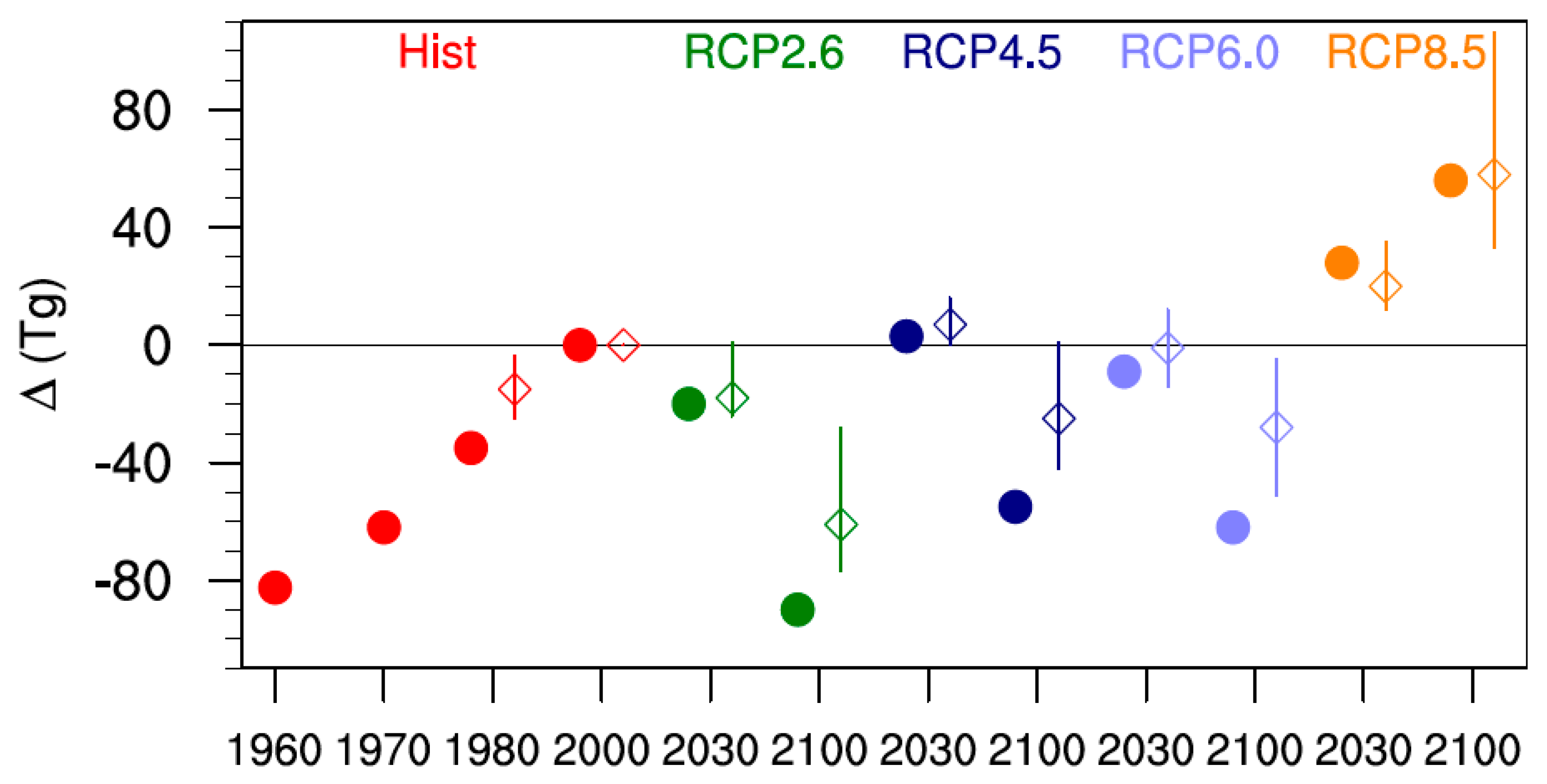
Figure 3.
Change in tropospheric ozone burden compared to the year 2000 as a function of (Left) changes in total NOx emissions and (Right) changes in the tropospheric CH4 burden as simulated by SOCOLv3. Different colors represent the different scenarios, whereas different symbols represent different years.

Figure 4.
Annual cycle of ozone at Arosa, Switzerland, for various decades. Observations are available for the 1950s and 2000s (solid lines), while SOCOL results are shown for the 1960s and 2000s (dashed lines). The SOCOL data are extracted from the 850 hPa level.
Figure 4.
Annual cycle of ozone at Arosa, Switzerland, for various decades. Observations are available for the 1950s and 2000s (solid lines), while SOCOL results are shown for the 1960s and 2000s (dashed lines). The SOCOL data are extracted from the 850 hPa level.
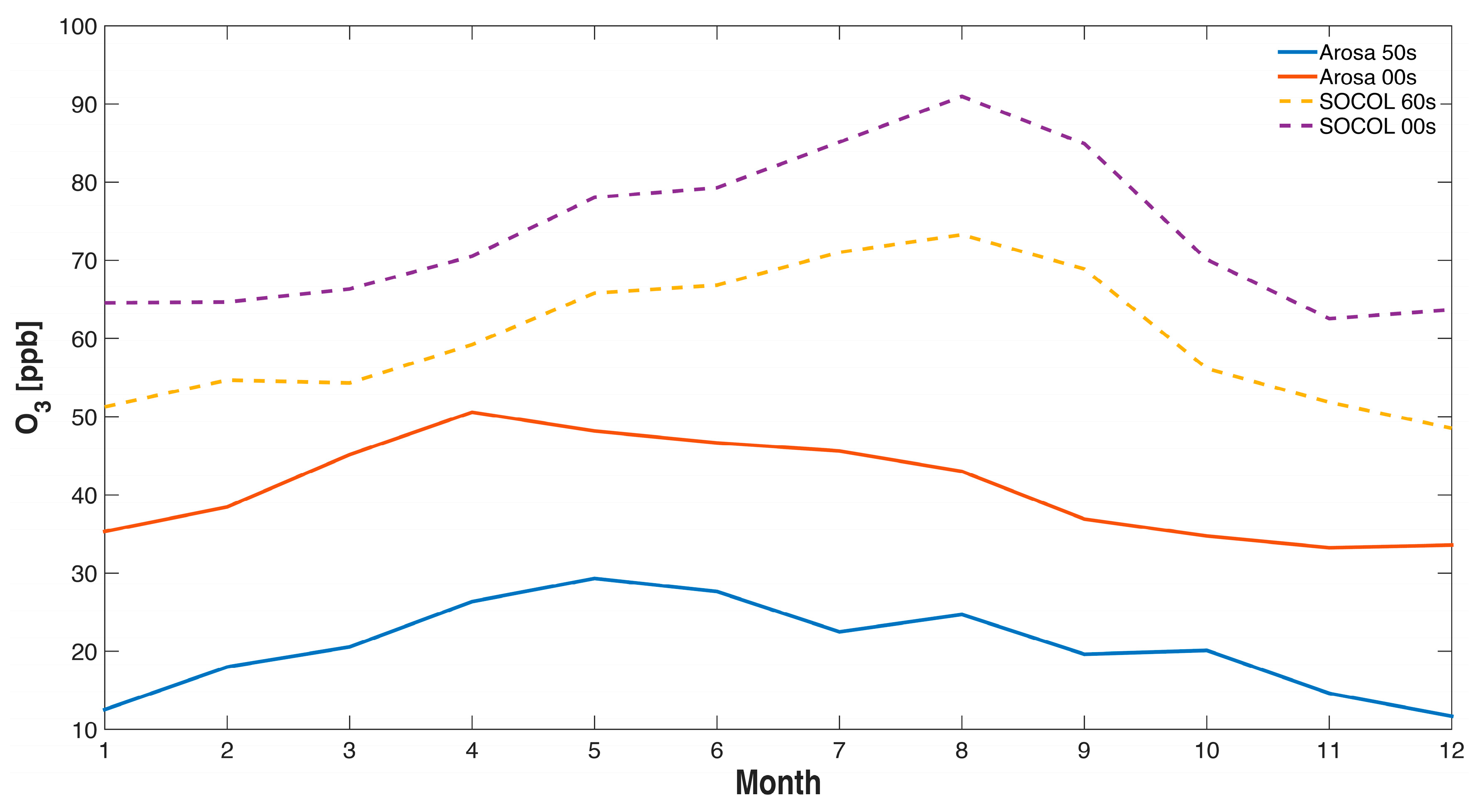
Figure 5.
Comparison of ozone measurements and the SOCOLv3 historical (REF-C1) simulation (annual mean values) at Arosa, Switzerland. The SOCOL data are extracted from the 850 hPa level. Note that the values for the years 1954–1958 are a multi-year mean and are thus the same for all years.
Figure 5.
Comparison of ozone measurements and the SOCOLv3 historical (REF-C1) simulation (annual mean values) at Arosa, Switzerland. The SOCOL data are extracted from the 850 hPa level. Note that the values for the years 1954–1958 are a multi-year mean and are thus the same for all years.

Figure 6.
Time series (monthly mean values) of (a) NOx; (b) CO; and (c) ozone for SOCOL (from 700 hPa level, blue) and observations (red). The NOx and CO observations are from Jungfraujoch (Switzerland), while the ozone time series is an average from Zugspitze (Germany), Jungfraujoch (Switzerland), and Sonnblick (Austria) (see text for details).

Figure 7.
Time series of historical (1960 to 2014) NOx emissions for Europe (blue) and Switzerland (red) as used in the SOCOLv3 simulations compared to NOx emissions reported by the Swiss Federal Office for Environment (FOEN, dashed black [72]). All values are shown relative to the year 1980.
Figure 7.
Time series of historical (1960 to 2014) NOx emissions for Europe (blue) and Switzerland (red) as used in the SOCOLv3 simulations compared to NOx emissions reported by the Swiss Federal Office for Environment (FOEN, dashed black [72]). All values are shown relative to the year 1980.


Table 1.
Regular aircraft measurements relevant for ozone and reactive gases in the troposphere.
| Name | Period | Flight Routes | Species |
|---|---|---|---|
| GASP | 1975–1979 | Pacific, Europe (Far East) | O3, others questionable |
| MOZAIC/IAGOS | Since 1994 | Various, starting from Europe | O3, H2O, and starting in 2001 also NOy (NOx + HNO3) and others |
| NOXAR | 1995/96, 97 | Zürich, Switzerland, to USA and Far East | O3 and NOx (=NO + NO2) |
| CARIBIC | Since 1997 | Various, from Frankfurt, Germany, monthly frequency | O3 and a large number of other species |
GASP: Global Atmospheric Sampling Program; MOZAIC/IAGOS: Measurement of Ozone and Water Vapor by Airbus In-Service Aircraft Program/In-service Aircraft for a Global Observing System; NOXAR: Nitrogen Oxides and ozone along Air Routes; CARIBIC: Civil Aircraft for the Regular Investigation of the atmosphere Based on an Instrument Container.
Table 2.
Summary of boundary conditions used in SOCOL simulations.
| Simulation | Period | Greenhouse Gases (CO2, N2O, CH4, ODSs) | Ozone Precursor Emissions (NOx, CO, NMVOCs) | Sea Surface Temperatures |
|---|---|---|---|---|
| REF-C1 | 1960–2010 | Observations until 2005 a then RCP 8.5 b | Historical emissions until 2000 c, then RCP6.0 | HadISST1 observations d |
| RCP 2.6 | 2000–2100 | Observations until 2005 then RCP 2.6 e | RCP 2.6 | CESM1(CAM5) f RCP 2.6 |
| RCP 4.5 | 2000–2100 | Observations until 2005 then RCP 4.5 g | RCP 4.5 | CESM1(CAM5) RCP 4.5 |
| RCP 6.0 | 1960–2100 | Observations until 2005 then RCP 6.0 h | Historical emissions until 2000 c, then RCP 6.0 | CESM1(CAM5) RCP 6.0 |
| RCP 8.5 | 2000–2100 | Observations until 2005 then RCP 8.5 b | RCP 8.5 | CESM1(CAM5) RCP 8.5 |
| NOx halved | 1960–1970 | As REF-C1 | As REF-C1, but NOx emissions halved | As REF-C1 |
| NOx & CO halved | 1960–1970 | As REF-C1 | As REF-C1, but NOx and CO emissions halved | As REF-C1 |
Table 3.
Tropospheric ozone burden (B) and budget statistics for SOCOLv3, and the ACCMIP and ACCENT model evaluations (mean ± stddev) for the year 2000. For SOCOL the 1995–2005 mean is shown. The 150 ppb ozone level is used to define the tropopause. The flux terms involve chemical production (P) and loss (L), dry deposition (D), and stratospheric influx (S). The stratospheric influx is calculated as a residual of production and loss terms (S = L + D − P) or directly using the ozone origin tracers. The lifetime τ is calculated as follows: τ = B/(L + D).
| Model | Burden (Tg(O3)) | Flux Terms (Tg(O3) year−1) | τ (Days) | |||
|---|---|---|---|---|---|---|
| P | L | D | S | |||
| SOCOL | 413 | 6857 a | 5597 b | 1500 | 240 (491 c) | 22.1 |
| ACCMIP | 337 ± 23 | 4877 ± 853 | 4260 ± 645 | 1094 ± 264 | 477 ± 96 | 23.4 ± 2.2 |
| ACCENT | 336 ± 27 | 5110 ± 606 | 4668 ± 27 | 1003 ± 200 | 552 ± 168 | 22.3 ± 2.0 |
a Sum of HO2 + NO, RO2 + NO; b Sum of O(1D) + H2O, HO2 + O3, OH + O3, C5H8 + O3; c Stratospheric influx calculated from ozone origin tracers [20].
© 2017 by the authors. Licensee MDPI, Basel, Switzerland. This article is an open access article distributed under the terms and conditions of the Creative Commons Attribution (CC BY) license (http://creativecommons.org/licenses/by/4.0/).
Share and Cite
MDPI and ACS Style
Staehelin, J.; Tummon, F.; Revell, L.; Stenke, A.; Peter, T. Tropospheric Ozone at Northern Mid-Latitudes: Modeled and Measured Long-Term Changes. Atmosphere 2017, 8, 163. https://doi.org/10.3390/atmos8090163
AMA Style
Staehelin J, Tummon F, Revell L, Stenke A, Peter T. Tropospheric Ozone at Northern Mid-Latitudes: Modeled and Measured Long-Term Changes. Atmosphere. 2017; 8(9):163. https://doi.org/10.3390/atmos8090163
Chicago/Turabian StyleStaehelin, Johannes, Fiona Tummon, Laura Revell, Andrea Stenke, and Thomas Peter. 2017. "Tropospheric Ozone at Northern Mid-Latitudes: Modeled and Measured Long-Term Changes" Atmosphere 8, no. 9: 163. https://doi.org/10.3390/atmos8090163
Note that from the first issue of 2016, this journal uses article numbers instead of page numbers. See further details here.