Emission Inventory of On-Road Transport in Bangkok Metropolitan Region (BMR) Development during 2007 to 2015 Using the GAINS Model


Abstract
:1. Introduction
- (1)
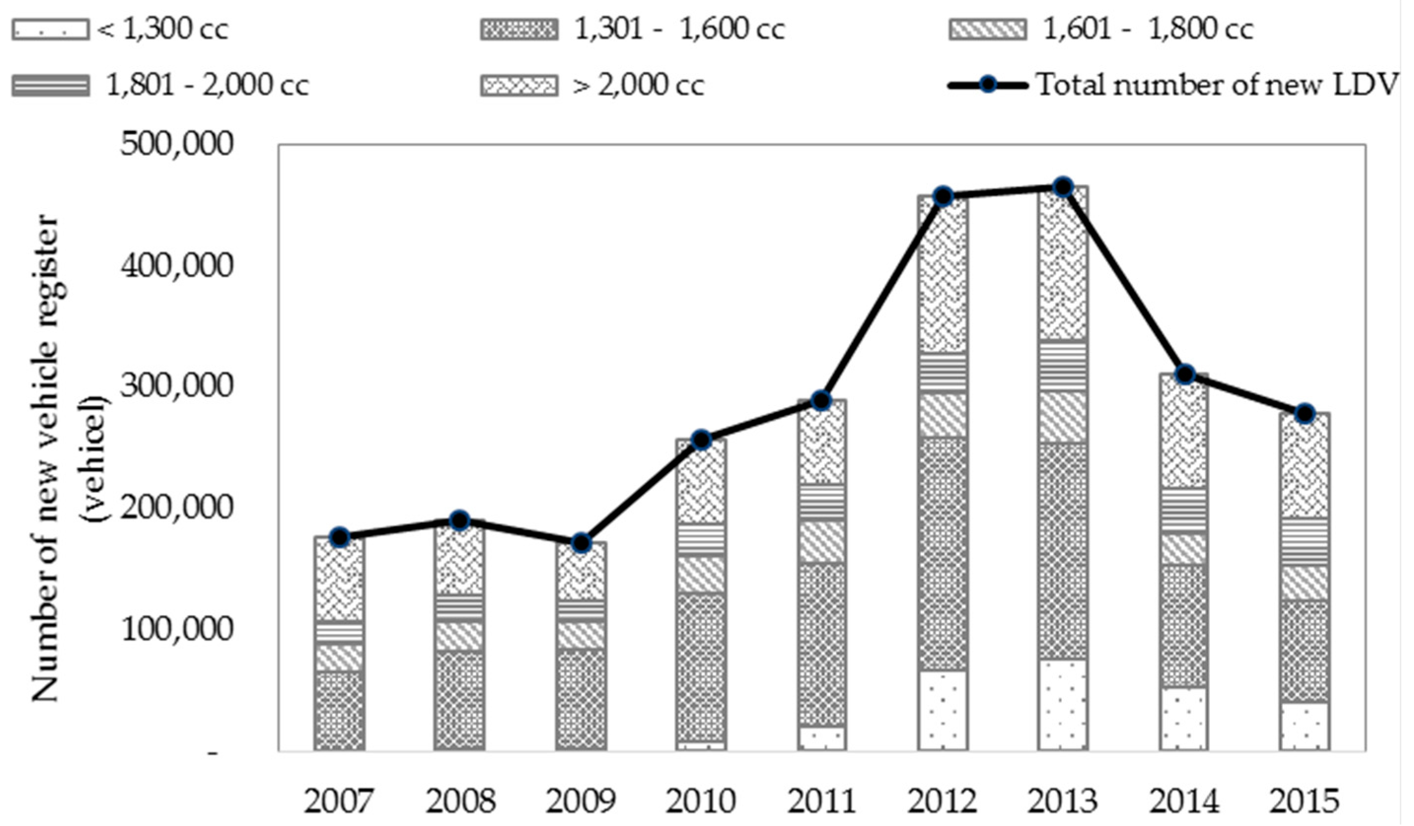
- “First car buyer incentive scheme”: Thailand launched this plan from 2011 to 2012. This scheme encouraged customers who did previously own a car to purchase a small engine car (less than 1500 cc engine). This scheme operated from 16 September 2011 to 31 December 2012, and the total vehicles sold under this plan was about 1.25 million; furthermore, more than half of the vehicles purchased under this plan were passenger cars (0.73 million vehicles). Of these passenger cars, about 44% (0.33 million vehicles) were registered in the BMR. It can be seen that this scheme had an impact on the sharp increase in the number of new vehicles [8].
- (2)
- “Eco car phase 1 and phase 2”: This plan operated in 2009 and 2015 for phase 1 and phase 2, respectively, with the objective of encouraging manufacturers to produce more efficient and environmental friendly vehicles, called ecology cars. Ecology cars are small cars (less than 1300 cc engine size for a gasoline engine and 1400 cc engine size for a diesel engine) which have high efficiency engines that meet the qualifications of Euro 4 engine standards. These plans influenced the sharp increase in small vehicles from 2389 cars in the year 2009 to 138, 592 cars in the year 2015 [9].
- (3)
- “Biofuel Development under Alternative Energy Development Plan 2015 (AEDP-2015)” [10]: Biofuel has been promoted as an alternative fuel for the transportation sector since the year 2001. Under AEDP-2015, the biofuel consumption target was set to use 14.0 million liters of biodiesel per day and 11.3 million liters of ethanol per day. A way to enhance the use of biofuel is to stop selling gasoline fuel and promote gasohol products (gasohol 91, gasohol 95, gasohol E20, and gasohol E85) instead. For biodiesel, an increase in higher blend products such as diesel B7 sold in the market has been seen since 2014.
- (4)
- “Oil Plan 2015”: Oil plan 2015 [11] aimed to support the use of LPG and NGV as an alternative fuel to substitute the use of benzene and diesel. For LPG consumption, the amount of LPG consumption has increased continuously. Taking into consideration the share of LPG consumption by sector, it was found that the growth rate of LPG consumed in the household sector has reduced since the year 2013 whereas the rate in the transportation sector has increased because the price of LPG is only 2 to 4 times cheaper than all gasohol products (except gasohol E85). The multi-fuel engine vehicle, known as a dual fuel vehicle, is a vehicle capable of running on two fuel types, one being gasoline or diesel and the other being an alternate fuel such as natural gas, LPG, or hydrogen. Dual fuel vehicles running gasoline and LPG has become popular since the fluctuation of petroleum fuel products. In addition, the financial incentive for choosing a gas-fueled system for both consumers and manufacturers is one cause of the sharp increase in duel fuel (petrol and LPG) vehicles, which rose from 0.16 million vehicles in 2007 to 1.00 million vehicles in 2015; more than half of which were registered in the BMR area [5]. For NGV consumption, Thailand has various plans that support the use of NGV as an equipped gas system in public transport systems such as buses and taxis, reducing the gas system installation cost, and expanding the gas station from 166 stations to 500 stations distributed around the country. In 2015, the cumulative number of duel fuel vehicles (petrol and NGV) registered was 0.186 million vehicles, of which 0.117 million vehicles or about 63% were registered in the BMR area [5].
- (5)
- “Fuel an Engine Quality Standard Enforcement”: Thailand has improved fuel quality in order to mitigate air pollution problems since 1983. The way to improve fuel quality is to limit the sulfur content and the aromatic hydrocarbon of the fuel. From Thailand, the air and noise pollution situation report presents the decrease of particulate matter and better ambient air quality especially in the BMR area; this is the result of the more intensive enforcement of fuel and engine standard levels, from the Euro 1 standard level in 1999 to the Euro 4 standard level in 2013 for light duty vehicles [12]. The qualification of engines at the Euro 4 standard level involves a stricter limit on CO, HC, and NOX for gasoline engines and on CO, NOX, HC + NOX, and PM for diesel engines compared to the previous standard. For fuel standard Euro 4, it has greater control on the content of aromatic hydrocarbon, olefin, and sulfur for gasoline fuel and polycyclic aromatic hydrocarbon (PAH) and sulfur content for diesel fuel [13]. Controlling at the Euro 4 standard level has resulted in the decreasing sulfur content in fuel up to 7–10 times compared to the previous standard, which reduced emissions of particulate matter 1732 tons per year, declining the particulate concentration 4.05 microgram per cubic meter [14]. However, the Pollution Control Department (PCD) under the Ministry of Natural Resources and Environment has a plan to further control the fuel and the engines of light duty vehicles at the Euro 5 level standard by 2020. Under the Euro 5 standard, the content of sulfur will be lower than 10 ppm; a 5-fold reduction compared to the Euro 4 standard. For motorcycles and heavy duty vehicles, the PCD plans to skip from the Euro 3 standard to the Euro 5 standard by 2019 and 2026, respectively [12].
2. Methodology
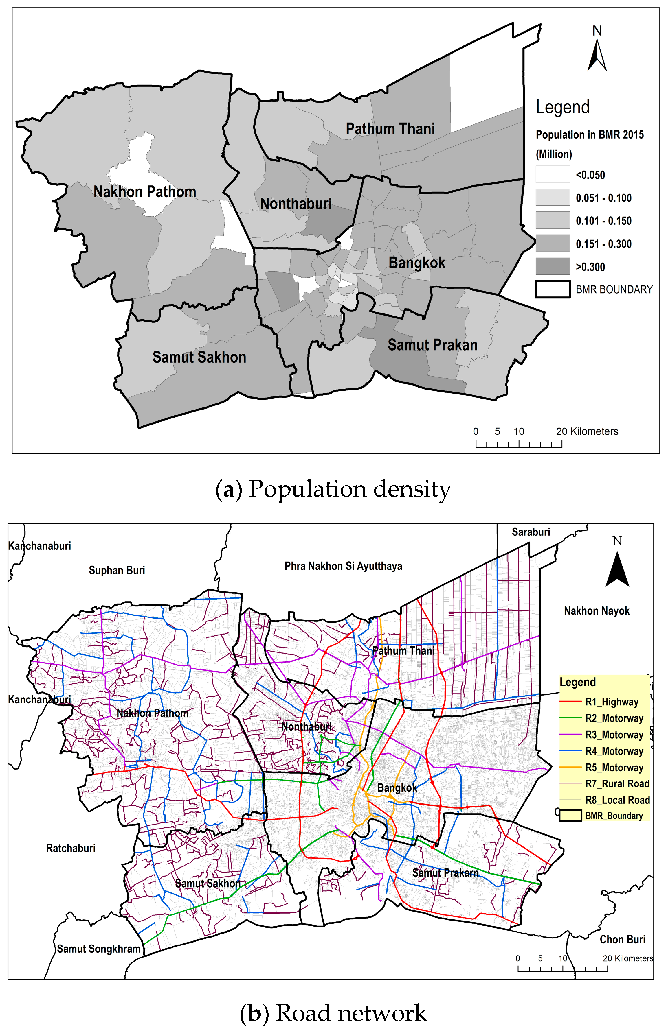
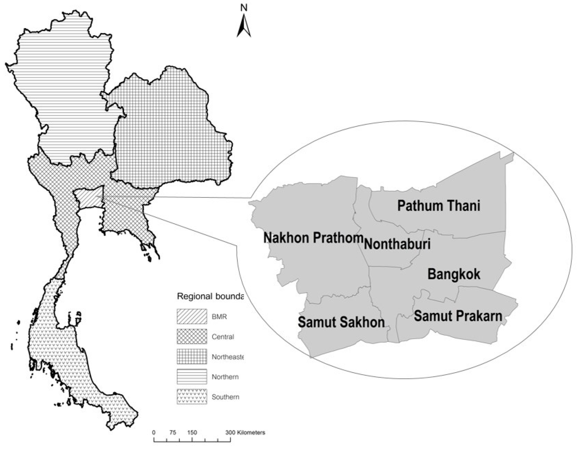
2.1. Site Study
2.2. Estimation of Emissions from the On-Road Transport Sector
2.2.1. Reference Method
2.2.2. GAINS Model Method
- i, s, f, t, p = country, sector, fuel, abatement technology, pollutant
- is the air emission of pollutant p in country i (kt)
- is the activity s (e.g., amount of fuel type f consumed) that produces pollutant i (PJ)
- is the uncontrolled emission factor (kt/PJ)
- is the application rate of technology t to activity s (dimensionless)
- is the no control emission factor for activity s (kt/PJ)
- is the removal efficiency of technology m when applied to activity s (dimensionless)
2.3. Data Used for the Estimation of Activity Data
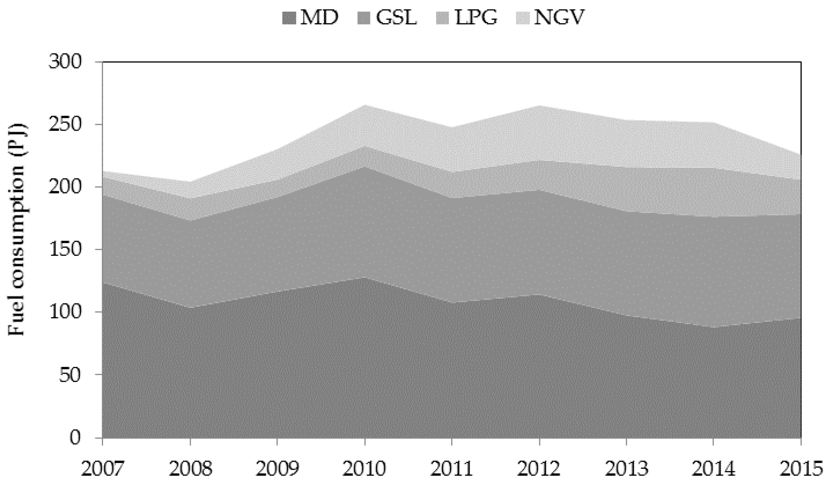
2.3.1. Basic Information of Fuel Consumption
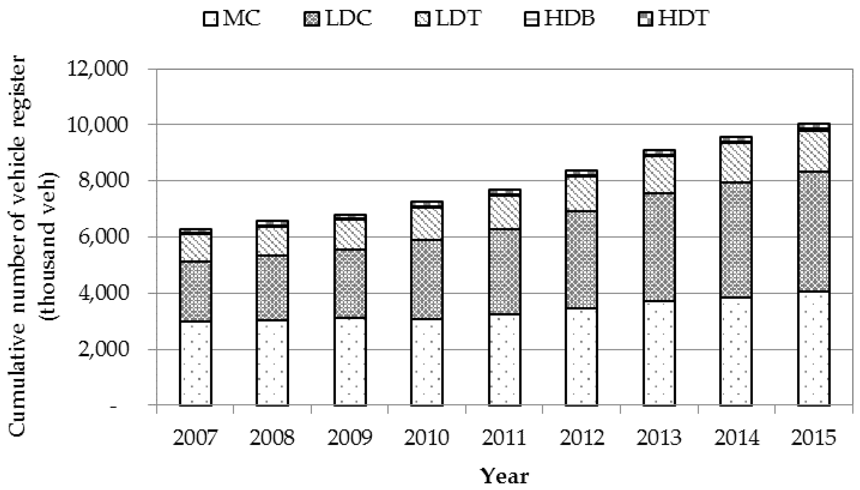
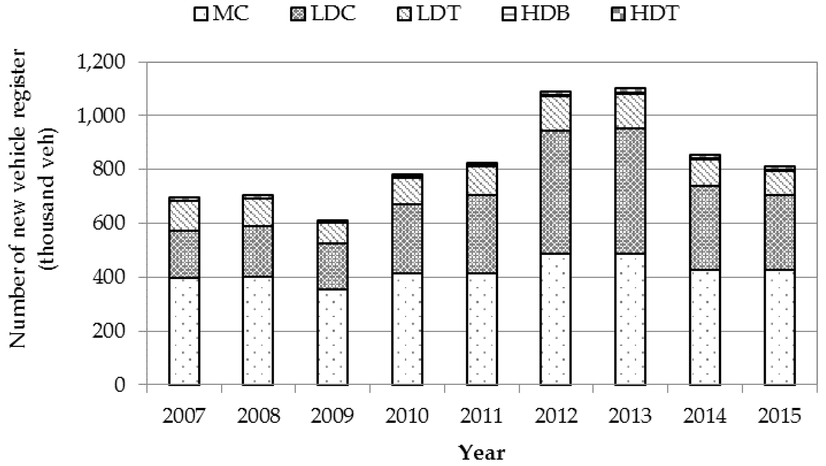
2.3.2. Cumulative Number of Vehicles Registered Classified by Vehicle and Fuel Types
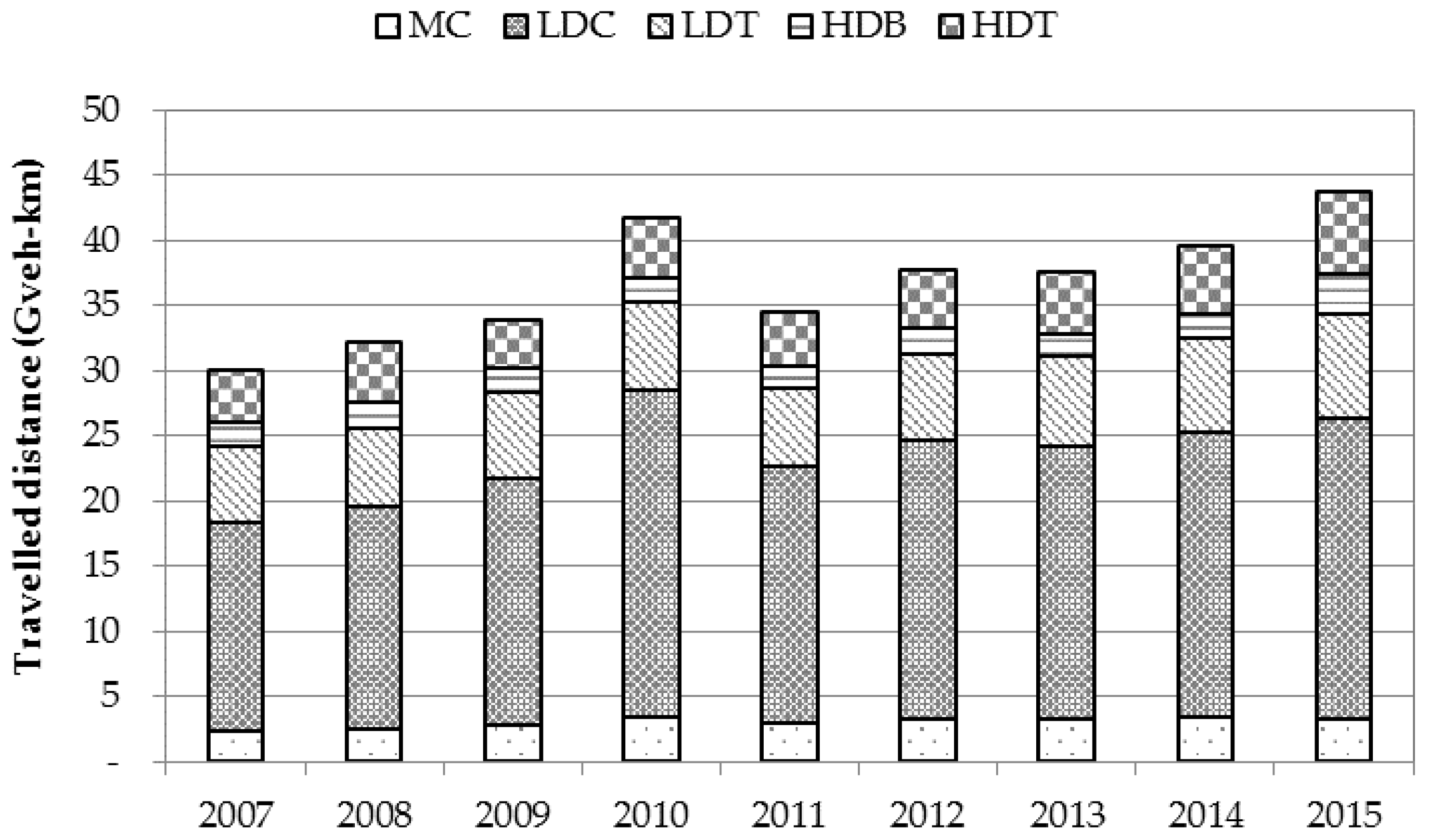
2.3.3. Distance Traveled by Vehicle Type
2.3.4. Fuel Economy of Each Vehicle Type
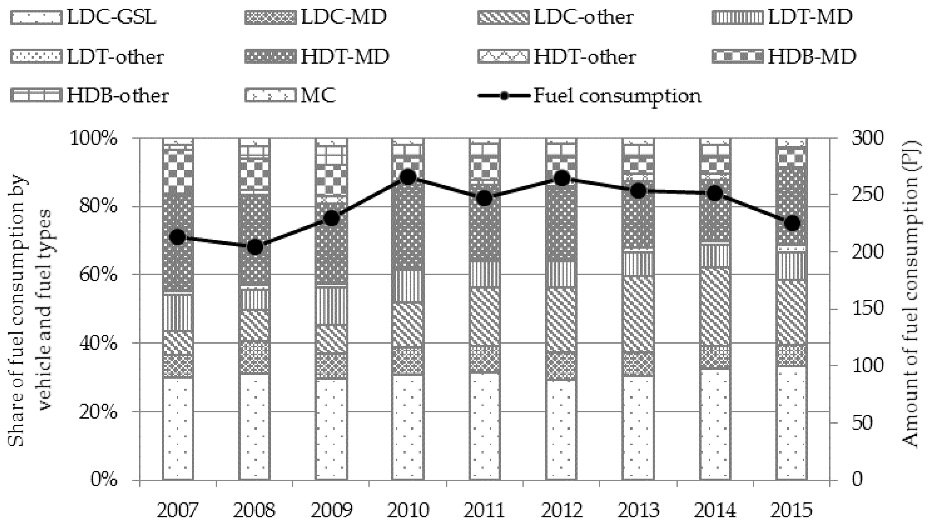
2.3.5. Fuel Consumption Disaggregate by Vehicle and Fuel Types
2.4. Emission Factors
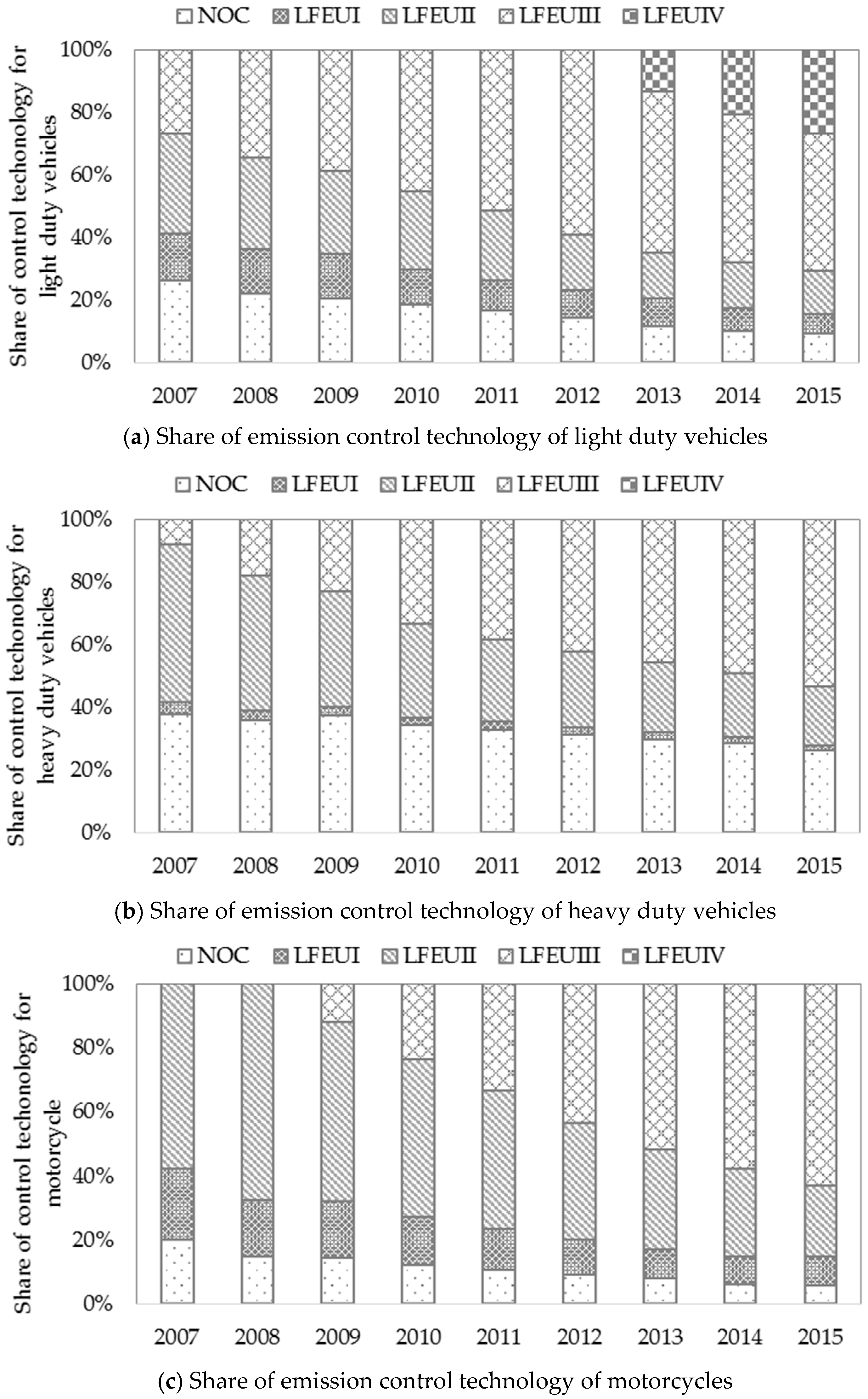
2.5. Control Technology
2.5.1. Exhaust Emission Regulation Enforcement
2.5.2. Share of Control Technology
2.6. Temporal and Spatial Variation of Exhaust Emission Determination
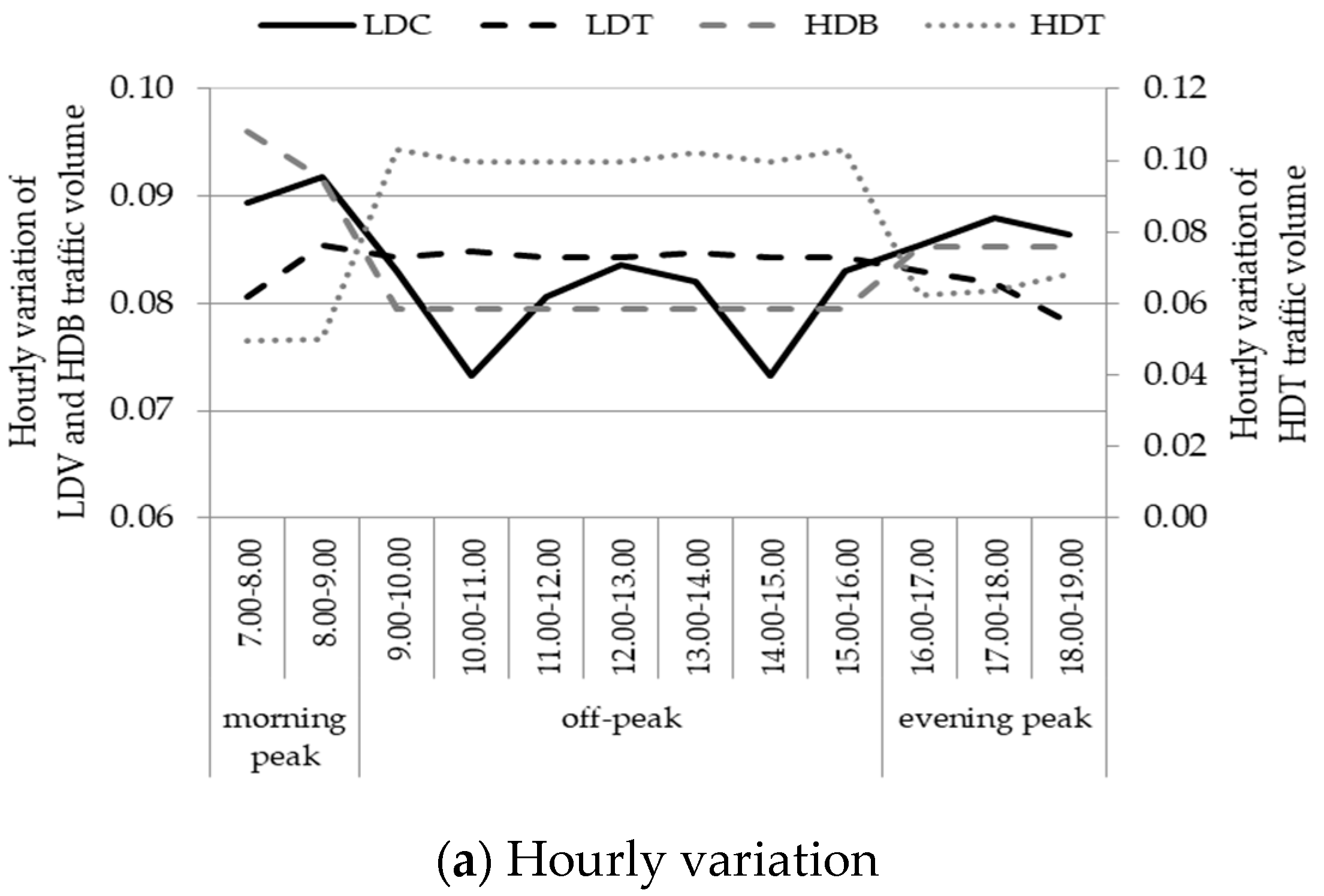
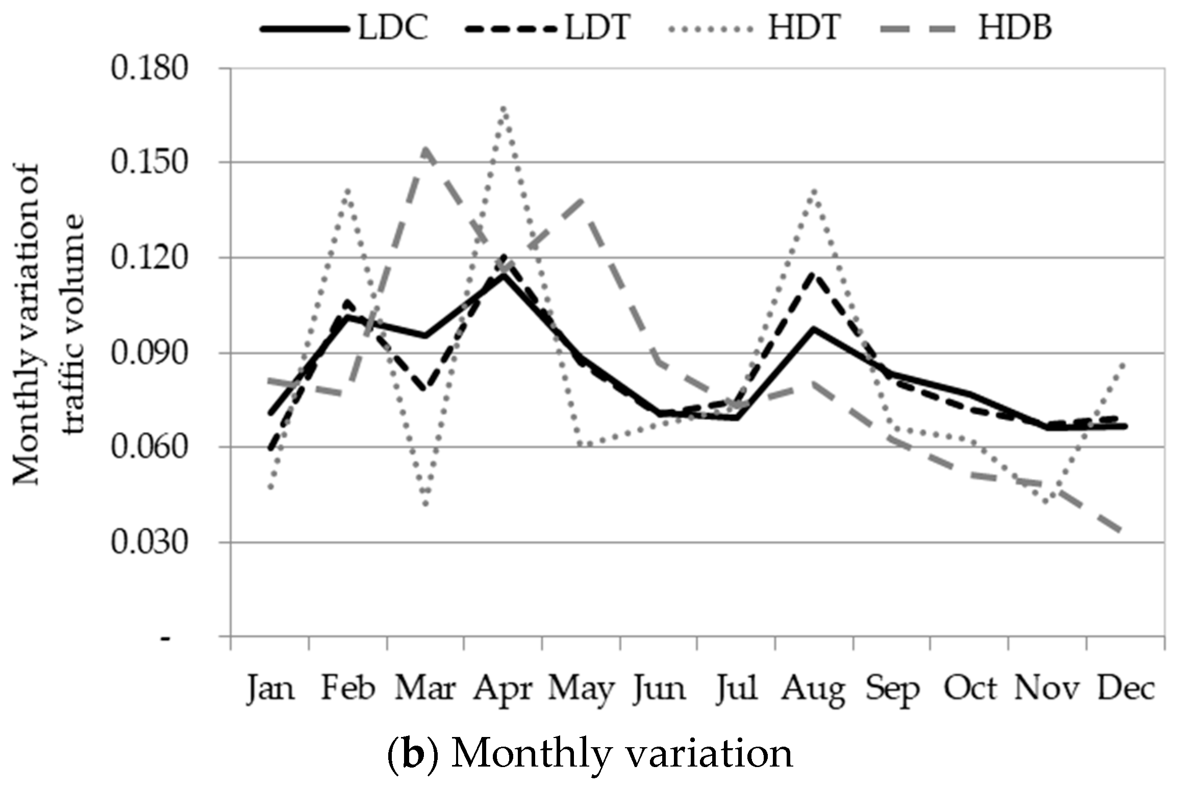
2.6.1. Temporal Variation of Traffic Demand
2.6.2. Spatial Variation of Traffic Demand
3. Results and Discussion
3.1. Emission Inventory from On-Road Transport in the BMR
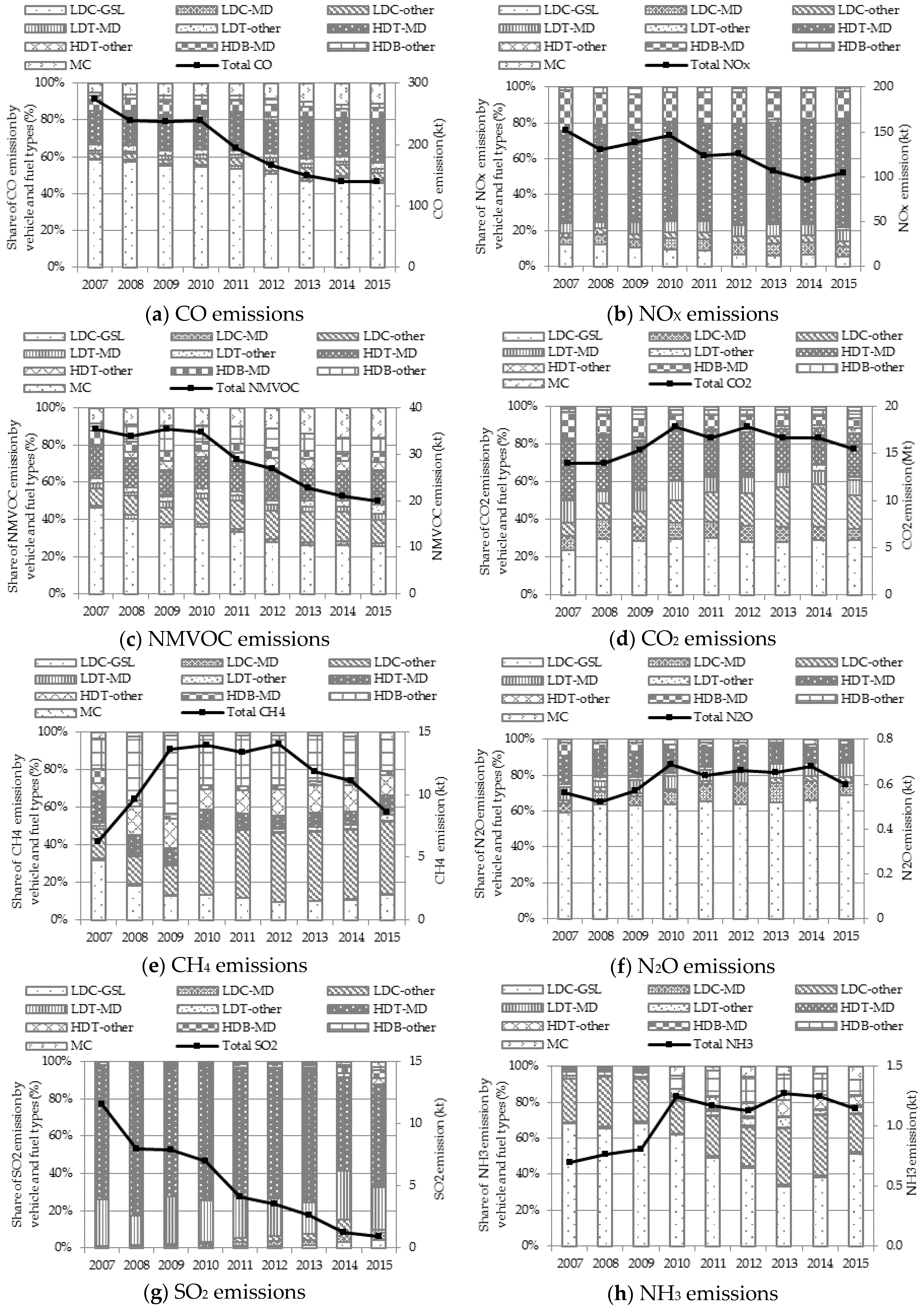
3.1.1. CO Emissions
3.1.2. NOX Emissions
3.1.3. NMVOC Emissions
3.1.4. CO2 Emissions
3.1.5. CH4 Emissions
3.1.6. N2O Emissions
3.1.7. SO2 Emissions
3.1.8. NH3 Emissions
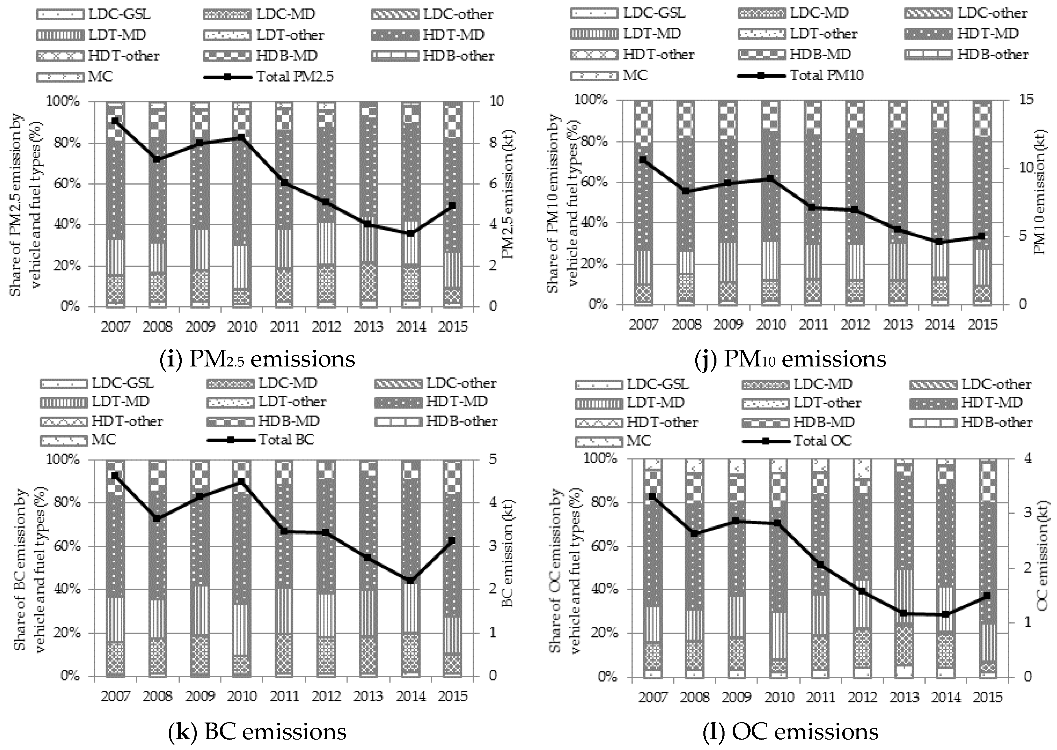
3.1.9. Particulate Matter (PM2.5, PM10, BC, and OC)
- (1)
- For PM2.5, the annual average from 2007 to 2015 was approximately 6.24 kt, the major contributor of which is heavy duty trucks, emitting an annual average 3.00 kt or a share of about 48% of the annual average of PM2.5; followed by light duty trucks (1.20 kt or 19% of the annual average), and light duty cars with diesel engine (0.83 kt or 13% of the annual average), and lastly heavy duty buses (0.82 kt or 13% of the annual average). The trend of PM2.5 showed a decrease from 9.07 kt in 2007 to 4.92 kt in 2015, with an average dropping rate of 5.5% annually.
- (2)
- For PM10, the annual average during the study period was about 7.38 kt. Heavy duty trucks dominates as the major emitter (3.88 kt or 53% of the annual average), followed by heavy duty buses (1.29 kt or 17.5% of the annual average) and light duty trucks (1.28 kt or 17.3% of the annual average). The trend of PM10 showed a decrease from 10.58 kt in 2007 to 5.05 kt in 2015, with an average dropping rate of 7.9% annually.
- (3)
- For BC, the annual average was about 3.51 kt, the major source of which is heavy duty trucks, followed by light duty trucks, and light duty cars with diesel engines at the average values of 1.73 kt (49% of the annual average), 0.74 kt (21% of the annual average), and 0.52 kt (15% of the annual average), respectively. The trend of BC showed a decrease from 4.62 kt in the year 2007 to 3.12 kt in the year 2015, with an average reduction rate of 2.5% annually.
- (4)
- For OC, the annual average was about 2.1 kt, the largest share of which comes from heavy duty trucks (0.96 kt or 45% of the annual average), followed by light duty trucks (0.39 kt or 18% of the annual average), and heavy duty buses (0.27 kt or 13% of the annual average), as well as light duty cars with diesel engine (0.26 kt or 13% of the annual average). The trend of OC showed a decrease from 3.92 kt in the year 2007 to 1.48 kt in the year 2015, with an average annual decreasing rate of 7.7%.
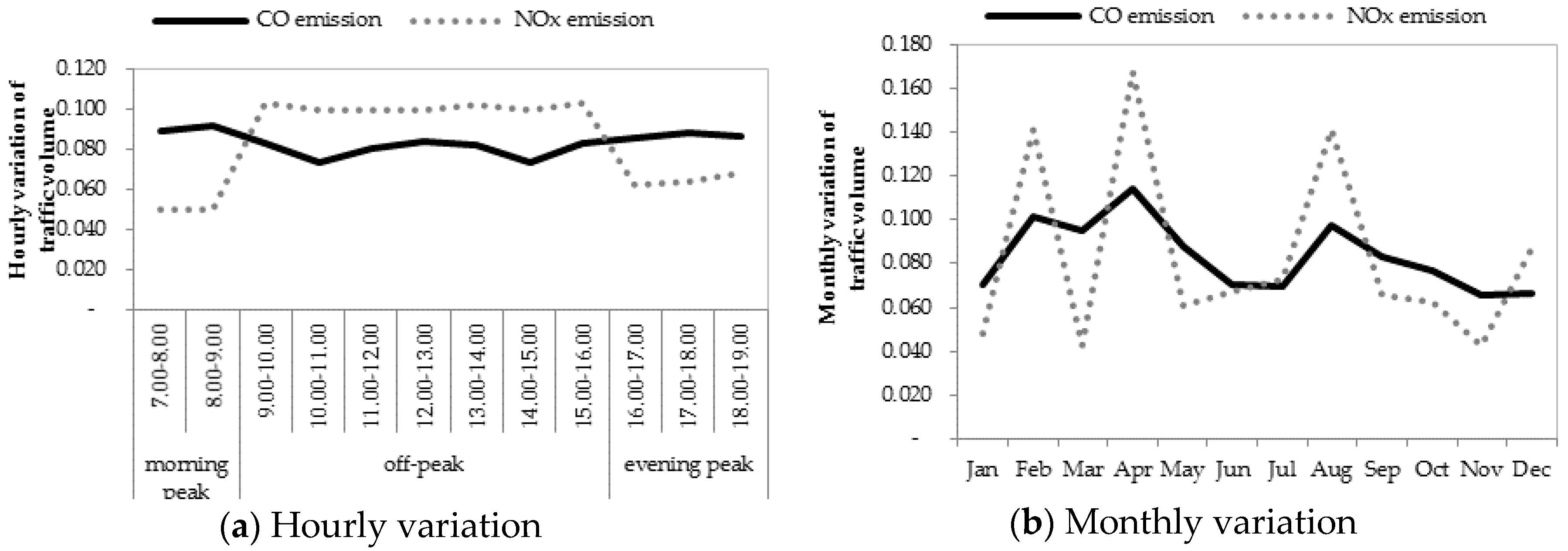
3.2. Temporal Distribution of Emissions from On-Road Transport
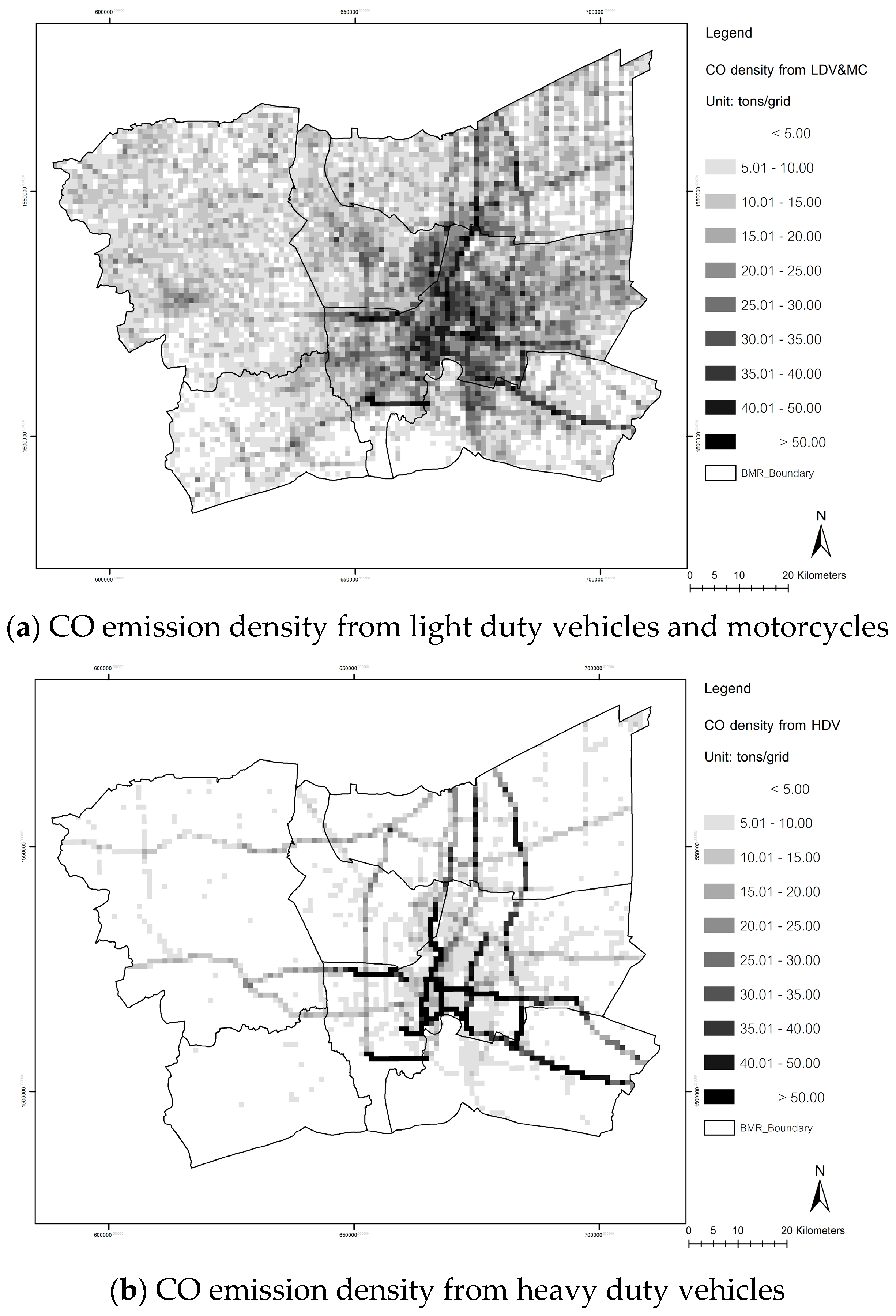
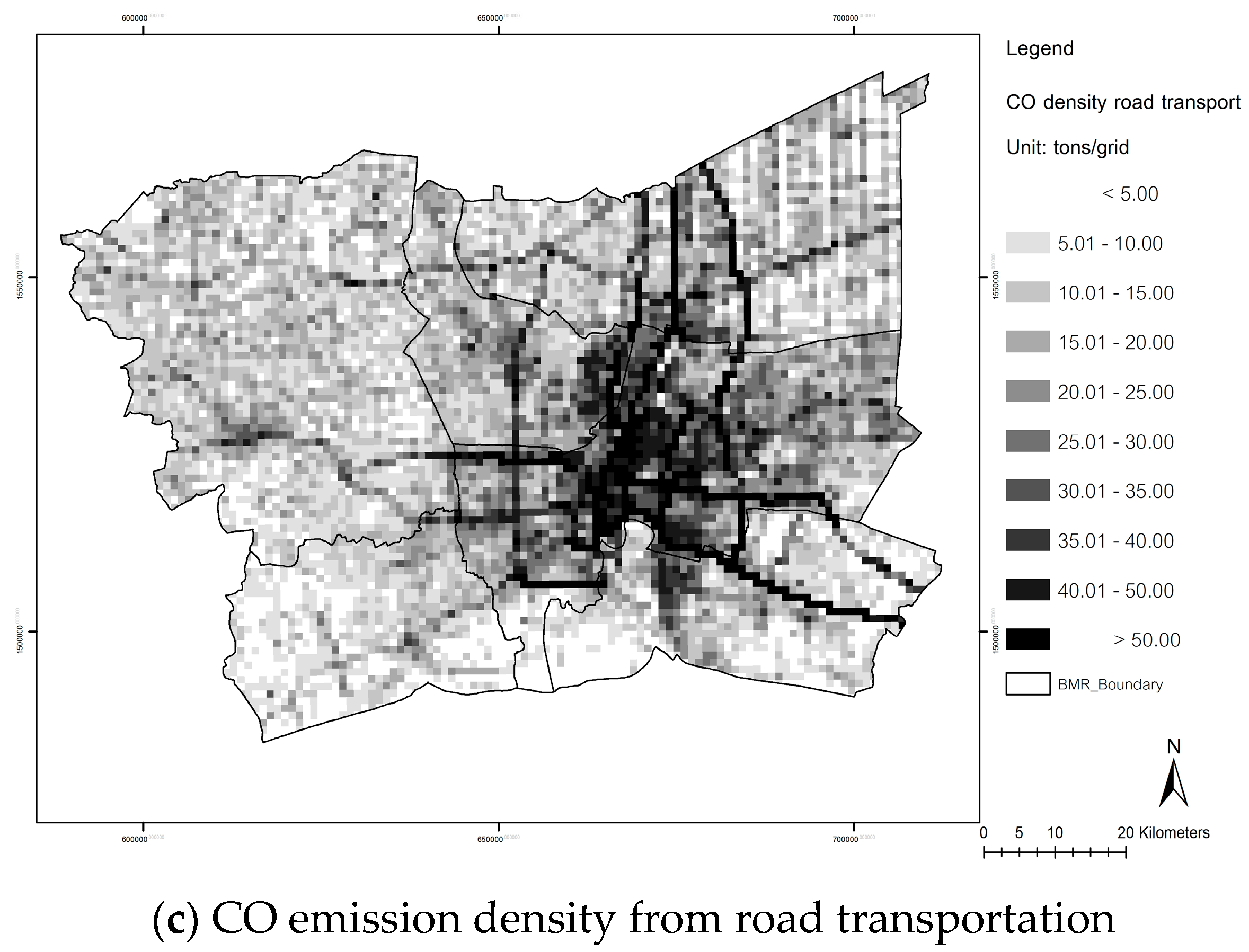
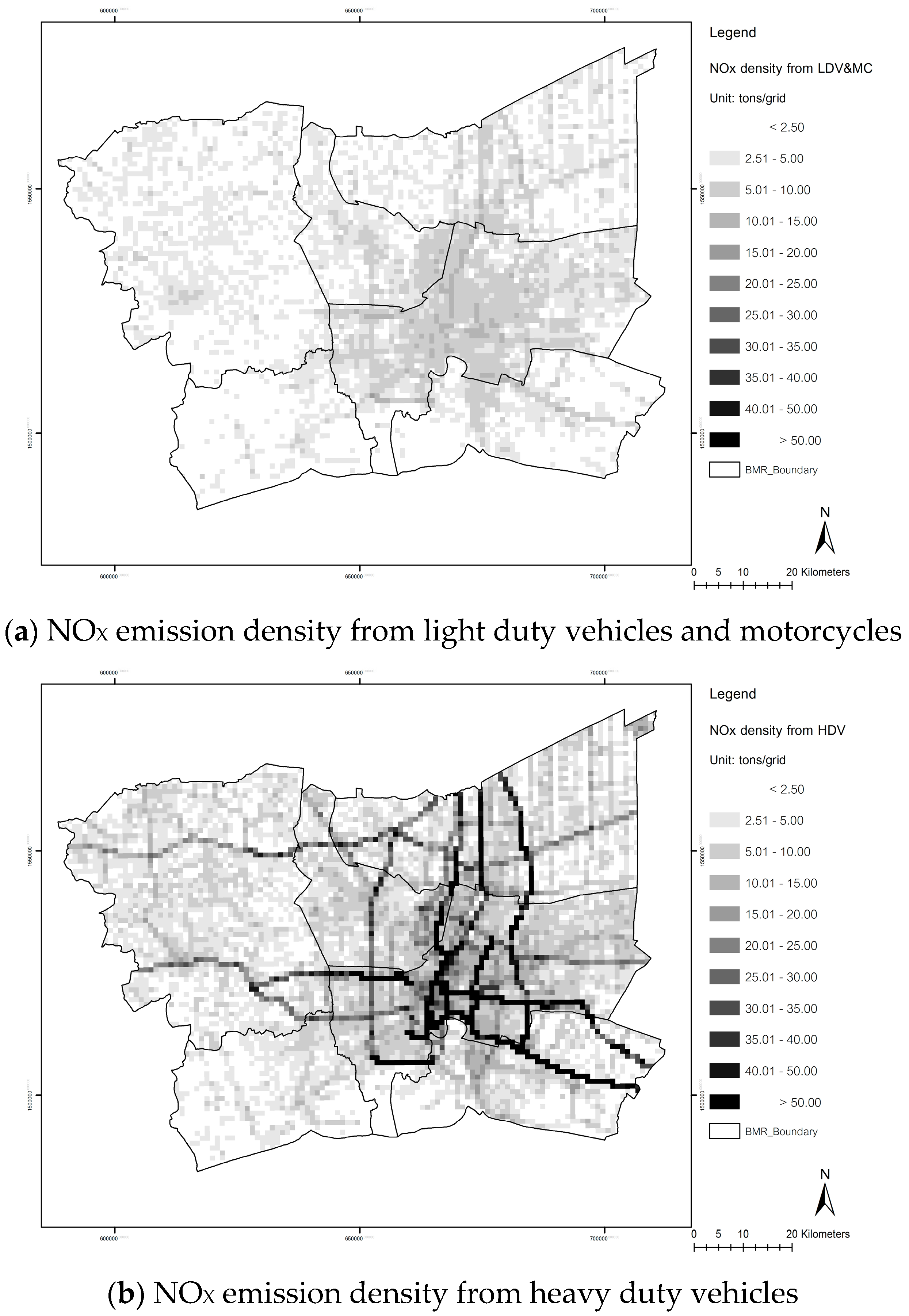
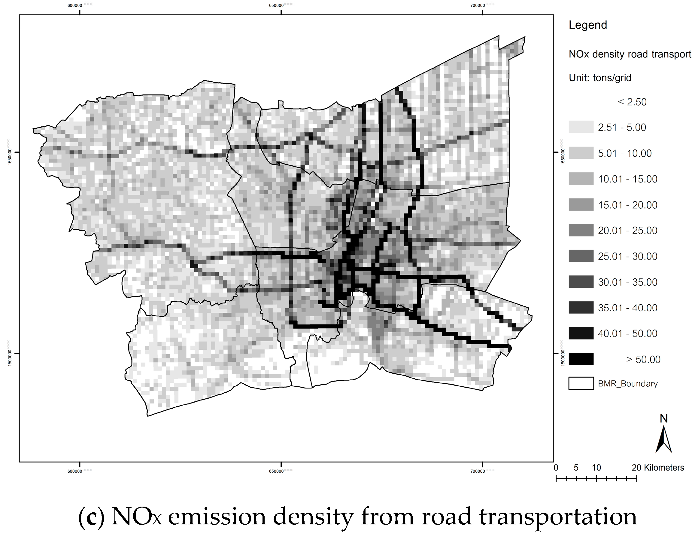
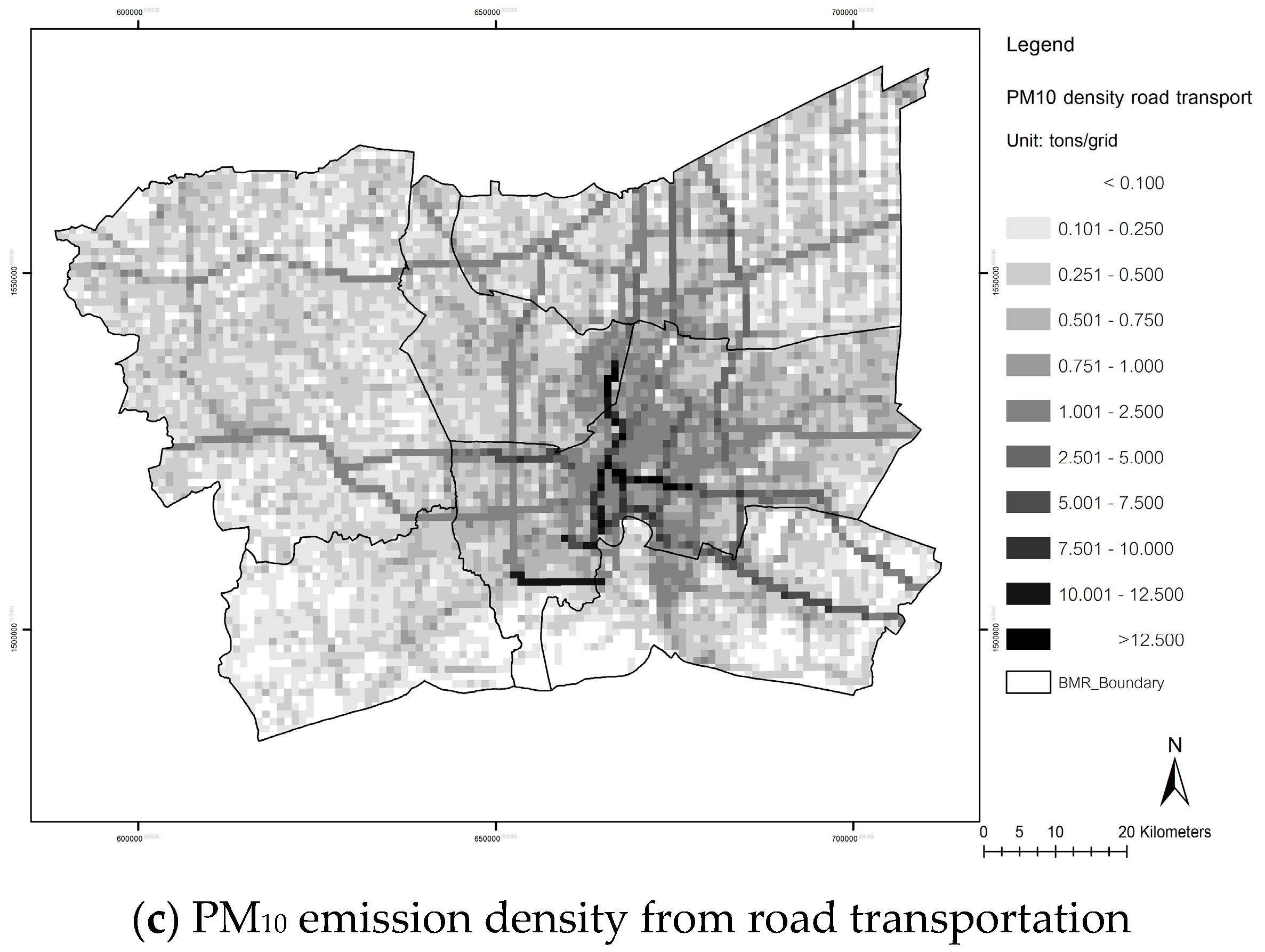
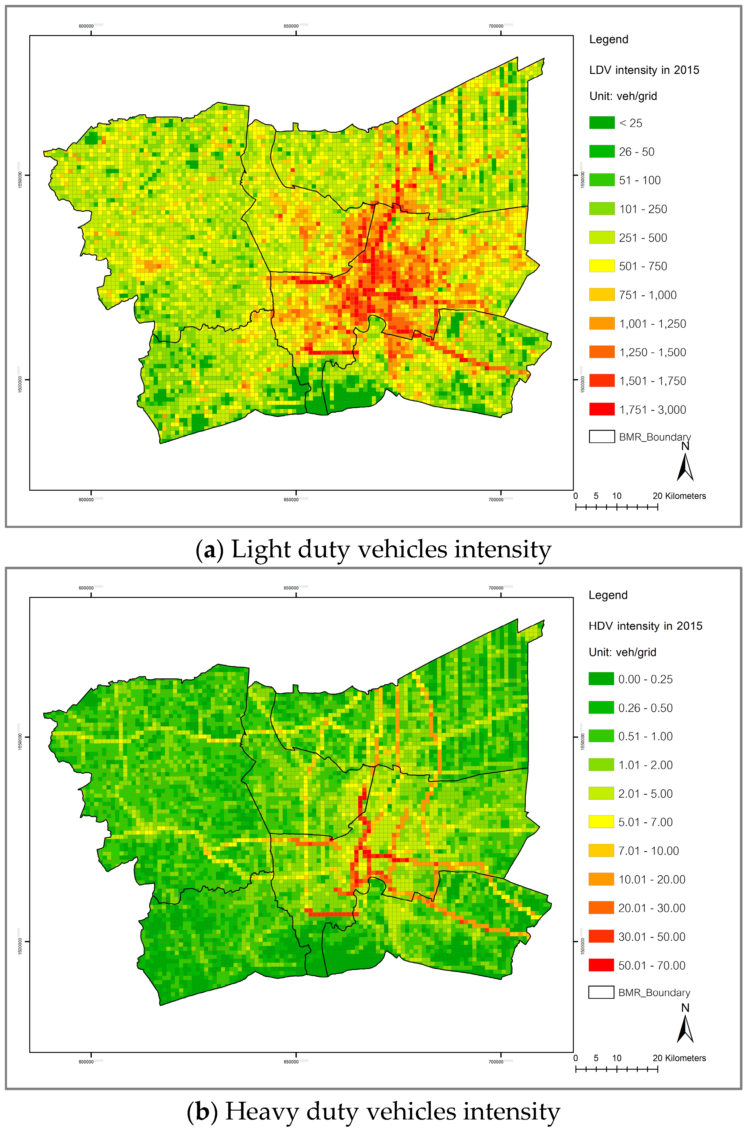
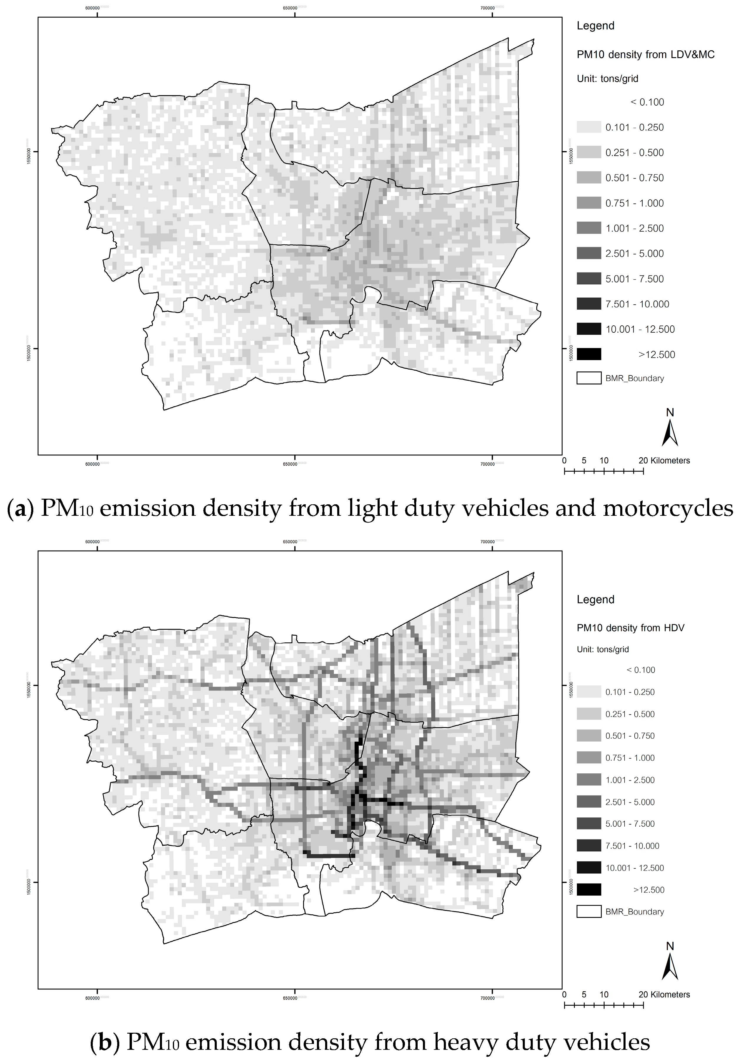
3.3. Spatial Distribution of Emissions from On-Road Transport
3.4 Comparison with Other Studies
4. Conclusions
Acknowledgments
Author Contributions
Conflicts of Interest
Appendix A

| (a) Emission Factor of Ozone Precursors (Unit: kt Emission/PJ) | |||||
| Vehicle-Fuel Types | Engine Standard | CO | NOX | NMVOC | |
| LDC/LDT-GSL | Pre-Euro | 6.9000 | 0.8600 | 0.7500 | |
| Euro 1 | 2.7600 | 0.2494 | 0.2175 | ||
| Euro 2 | 0.8280 | 0.1118 | 0.0975 | ||
| Euro 3 | 0.8280 | 0.0688 | 0.0600 | ||
| Euro 4 | 0.4830 | 0.0344 | 0.0300 | ||
| LDC/LDT-MD | Pre-Euro | 0.3100 | 0.3500 | 0.0600 | |
| Euro 1 | 0.2573 | 0.3675 | 0.0384 | ||
| Euro 2 | 0.1116 | 0.3850 | 0.0342 | ||
| Euro 3 | 0.1116 | 0.4025 | 0.0276 | ||
| Euro 4 | 0.1116 | 0.3850 | 0.0204 | ||
| LDC/LDT-LPG | Pre-Euro | 1.4500 | 0.8600 | 0.6375 | |
| Euro 1 | 0.5800 | 0.2494 | 0.1848 | ||
| Euro 2 | 0.1740 | 0.1118 | 0.0828 | ||
| Euro 3 | 0.1740 | 0.0688 | 0.0510 | ||
| Euro 4 | 0.1015 | 0.0344 | 0.0255 | ||
| LDC/LDT-NGV | Pre-Euro | 0.7200 | 0.6500 | 0.6500 | |
| Euro 1 | 0.2880 | 0.1885 | 0.1885 | ||
| Euro 2 | 0.0864 | 0.0845 | 0.0845 | ||
| Euro 3 | 0.0864 | 0.0520 | 0.0520 | ||
| Euro 4 | 0.0504 | 0.0260 | 0.0260 | ||
| HDT/HDB-GSL | Pre-Euro | 7.9000 | 0.8600 | 0.6500 | |
| Euro 1 | 1.1850 | 0.1548 | 0.1300 | ||
| Euro 2 | 0.9480 | 0.0860 | 0.0520 | ||
| Euro 3 | 0.9480 | 0.0602 | 0.0195 | ||
| Euro 4 | 0.9480 | 0.0602 | 0.0195 | ||
| HDT/HDB-MD | Pre-Euro | 0.9000 | 1.3000 | 0.1200 | |
| Euro 1 | 0.8550 | 1.2350 (HDT)/1.3000 (HDB) | 0.0840 | ||
| Euro 2 | 0.7560 | 1.1700 (HDT)/1.3000 (HDB) | 0.0612 | ||
| Euro 3 | 0.4050 | 1.1700 (HDT)/1.3000 (HDB) | 0.0516 | ||
| Euro 4 | 0.3240 | 0.8450 (HDT)/1.3000 (HDB) | 0.0516 | ||
| HDT/HDB-LPG | Pre-Euro | 1.5200 | 0.8600 | 0.5525 | |
| Euro 1 | 0.2280 | 0.1548 | 0.1105 | ||
| Euro 2 | 0.1824 | 0.0860 | 0.0442 | ||
| Euro 3 | 0.1824 | 0.0602 | 0.01657 | ||
| Euro 4 | 0.1824 | 0.0602 | 0.01657 | ||
| HDT/HDB-NGV | Pre-Euro | 0.7400 | 0.6500 | 0.5600 | |
| Euro 1 | 0.1110 | 0.1170 | 0.1120 | ||
| Euro 2 | 0.0888 | 0.0650 | 0.0448 | ||
| Euro 3 | 0.0888 | 0.0455 | 0.0168 | ||
| Euro 4 | 0.0888 | 0.0455 | 0.0168 | ||
| MC | Pre-Euro | 12.000 | 0.1300 | 1.3430 | |
| Euro 1 | 7.2000 | 0.1300 | 1.2758 | ||
| Euro 2 | 3.0000 | 0.1157 | 0.5506 | ||
| Euro 3 | 1.2000 | 0.0585 | 0.1745 | ||
| (b) Emission Factor of GHG Emissions (Unit: kt Emission/PJ) | |||||
| Vehicle-Fuel Types | Engine Standard | CO2 | N2O | CH4 | |
| LDC/LDT-GSL | Pre-Euro | 68,600 | 0.0031 | 0.0690 | |
| Euro 1 | - | 0.0136 | 0.0150 | ||
| Euro 2 | - | 0.0055 | 0.0210 | ||
| Euro 3 | - | 0.0055 | 0.0160 | ||
| Euro 4 | - | 0.0055 | 0.0110 | ||
| LDC/LDT-MD | Pre-Euro | 73,400 | 0.0018 | 0.0093 | |
| Euro 1 | - | 0.0018 | 0.0056 | ||
| Euro 2 | - | 0.0018 | 0.0023 | ||
| Euro 3 | - | 0.0018 | 0.0016 | ||
| Euro 4 | - | 0.0052 | 0.0000 | ||
| LDC/LDT-LPG | Pre-Euro | 68,600 | 0.0006 | 0.0332 | |
| Euro 1 | - | - | 0.0332 | ||
| Euro 2 | - | - | 0.0332 | ||
| Euro 3 | - | - | 0.0332 | ||
| Euro 4 | - | - | 0.0332 | ||
| LDC/LDT-NGV | Pre-Euro | 55,800 | 0.0001 | 0.7000 | |
| Euro 1 | - | - | 0.1518 | ||
| Euro 2 | - | - | 0.2067 | ||
| Euro 3 | - | - | 0.1400 | ||
| Euro 4 | - | - | 0.0913 | ||
| HDT/HDB-GSL | Pre-Euro | 68,600 | 0.0031 | 0.0541 | |
| Euro 1 | - | - | 0.0117 | ||
| Euro 2 | - | - | 0.0160 | ||
| Euro 3 | - | - | 0.0108 | ||
| Euro 4 | - | - | 0.0108 | ||
| HDT/HDB-MD | Pre-Euro | 73,400 | 0.00180 | 0.0176 | |
| Euro 1 | - | 0.00106 | 0.0176 | ||
| Euro 2 | - | 0.00102 | 0.0176 | ||
| Euro 3 | - | 0.00061 | 0.0176 | ||
| Euro 4 | - | 0.00310 | 0.0176 | ||
| HDT/HDB-LPG | Pre-Euro | 68,600 | 0.0006 | 0.0092 | |
| Euro 1 | - | - | 0.0092 | ||
| Euro 2 | - | - | 0.0092 | ||
| Euro 3 | - | - | 0.0092 | ||
| Euro 4 | - | - | 0.0092 | ||
| HDT/HDB-NGV | Pre-Euro | 55,800 | 0.0001 | 0.6531 | |
| Euro 1 | - | - | 0.1419 | ||
| Euro 2 | - | - | 0.1930 | ||
| Euro 3 | - | - | 0.1306 | ||
| Euro 4 | - | - | 0.1306 | ||
| MC | Pre-Euro | 68,600 | 0.0031 | 0.0590 | |
| Euro 1 | - | - | 0.0590 | ||
| Euro 2 | - | - | 0.0590 | ||
| Euro 3 | - | - | 0.0590 | ||
| (c) Emission Factor of Acidic Substance (Unit: kt Emission/PJ) | |||||
| Vehicle-Fuel Types | Engine Standard | SO2 | NH3 | ||
| LDC/LDT-GSL | Pre-Euro | 0.0091 | 0.00073 | ||
| Euro 1 | 0.0004 | 0.03000 | |||
| Euro 2 | - | 0.01200 | |||
| Euro 3 | - | 0.01200 | |||
| Euro 4 | - | 0.00210 | |||
| LDC/LDT-MD | Pre-Euro | 0.4608 | 0.00045 | ||
| Euro 1 | 0.0921 | 0.00045 | |||
| Euro 2 | 0.0207 | 0.00040 | |||
| Euro 3 | 0.0004 | 0.00040 | |||
| Euro 4 | - | 0.00100 | |||
| LDC/LDT-LPG | Pre-Euro | 0.0042 | 0.00073 | ||
| Euro 1 | - | 0.03000 | |||
| Euro 2 | - | 0.01200 | |||
| Euro 3 | - | 0.01200 | |||
| Euro 4 | - | 0.00210 | |||
| LDC/LDT-NGV | Pre-Euro | - | 0.00050 | ||
| Euro 1 | - | 0.00490 | |||
| Euro 2 | - | 0.00490 | |||
| Euro 3 | - | 0.00300 | |||
| Euro 4 | - | 0.00250 | |||
| HDT/HDB-GSL | Pre-Euro | 0.0091 | 0.00026 | ||
| Euro 1 | 0.0004 | 0.01100 | |||
| Euro 2 | 0.0004 | 0.01000 | |||
| Euro 3 | 0.0004 | 0.00500 | |||
| Euro 4 | 0.0004 | 0.00500 | |||
| HDT/HDB-MD | Pre-Euro | 0.4608 | 0.00029 | ||
| Euro 1 | 0.0921 | 0.00029 | |||
| Euro 2 | 0.0207 | 0.00025 | |||
| Euro 3 | 0.0004 | 0.00025 | |||
| Euro 4 | 0.0004 | 0.00045 | |||
| HDT/HDB-LPG | Pre-Euro | 0.0042 | 0.00026 | ||
| Euro 1 | - | 0.01100 | |||
| Euro 2 | - | 0.01000 | |||
| Euro 3 | - | 0.00500 | |||
| Euro 4 | - | 0.00500 | |||
| HDT/HDB-NGV | Pre-Euro | - | 0.00050 | ||
| Euro 1 | - | 0.01000 | |||
| Euro 2 | - | 0.00500 | |||
| Euro 3 | - | 0.00500 | |||
| Euro 4 | - | 0.00500 | |||
| MC | Pre-Euro | 0.0091 | 0.00100 | ||
| Euro 1 | 0.0004 | 0.03500 | |||
| Euro 2 | - | 0.01500 | |||
| Euro 3 | - | 0.01500 | |||
| (d) Emission Factor of Particulate Matter (Unit: kt Emission/PJ) | |||||
| Vehicle-Fuel Types | Engine Standard | PM2.5 | PM10 | BC | OC |
| LDC/LDT-GSL | Pre-Euro | 0.00597 | 0.00630 | 0.00099 | 0.00330 |
| Euro 1 | 0.00328 | 0.00347 | 0.00091 | 0.00162 | |
| Euro 2 | 0.00328 | 0.00347 | 0.00091 | 0.00162 | |
| Euro 3 | 0.00107 | 0.00113 | 0.00052 | 0.00036 | |
| Euro 4 | 0.00107 | 0.00113 | 0.00049 | 0.00036 | |
| LDC/LDT-MD | Pre-Euro | 0.10467 | 0.10940 | 0.05757 | 0.03977 |
| Euro 1 | 0.10467 | 0.10940 | 0.05757 | 0.03977 | |
| Euro 2 | 0.08897 | 0.09299 | 0.05354 | 0.03182 | |
| Euro 3 | 0.01995 | 0.02085 | 0.01693 | 0.00251 | |
| Euro 4 | 0.01945 | 0.02033 | 0.01692 | 0.00217 | |
| LDC/LDT-LPG | Pre-Euro | 0.00184 | 0.00198 | 0.00300 | 0.00100 |
| Euro 1 | 0.00101 | 0.00109 | 0.00028 | 0.00049 | |
| Euro 2 | 0.00101 | 0.00109 | 0.00028 | 0.00049 | |
| Euro 3 | 0.00033 | 0.00036 | 0.00016 | 0.00049 | |
| Euro 4 | 0.00033 | 0.00036 | 0.00016 | 0.00011 | |
| LDC/LDT-NGV | Pre-Euro | 0.00184 | 0.00200 | 0.00300 | 0.00100 |
| Euro 1 | 0.00101 | 0.00110 | 0.00028 | 0.00049 | |
| Euro 2 | 0.00101 | 0.00110 | 0.00028 | 0.00049 | |
| Euro 3 | 0.00033 | 0.00036 | 0.00016 | 0.00049 | |
| Euro 4 | 0.00033 | 0.00036 | 0.00015 | 0.00011 | |
| HDT/HDB-GSL | Pre-Euro | 0.02396 | 0.02531 | 0.00398 | 0.01325 |
| Euro 1 | 0.01318 | 0.01392 | 0.00364 | 0.00649 | |
| Euro 2 | 0.00431 | 0.00456 | 0.00210 | 0.00143 | |
| Euro 3 | 0.00407 | 0.00430 | 0.00198 | 0.00135 | |
| Euro 4 | 0.00407 | 0.00430 | 0.00198 | 0.00135 | |
| HDT/HDB-MD | Pre-Euro | 0.10659 | 0.10857 | 0.05330 | 0.03731 |
| Euro 1 | 0.07142 | 0.07274 | 0.05276 | 0.01865 | |
| Euro 2 | 0.04415 | 0.04497 | 0.03031 | 0.01006 | |
| Euro 3 | 0.02665 | 0.02714 | 0.02532 | 0.00666 | |
| Euro 4 | 0.00713 | 0.00726 | 0.00533 | 0.00117 | |
| HDT/HDB-LPG | Pre-Euro | 0.00184 | 0.00200 | 0.00030 | 0.00100 |
| Euro 1 | 0.00101 | 0.00110 | 0.00028 | 0.00049 | |
| Euro 2 | 0.00033 | 0.00036 | 0.00016 | 0.00011 | |
| Euro 3 | 0.00031 | 0.00034 | 0.00015 | 0.00010 | |
| Euro 4 | 0.00031 | 0.00034 | 0.00015 | 0.00010 | |
| HDT/HDB-NGV | Pre-Euro | 0.00184 | 0.00200 | 0.00030 | 0.00100 |
| Euro 1 | 0.00101 | 0.00110 | 0.00028 | 0.00049 | |
| Euro 2 | 0.00033 | 0.00036 | 0.00016 | 0.00011 | |
| Euro 3 | 0.00031 | 0.00034 | 0.00015 | 0.00010 | |
| Euro 4 | 0.00031 | 0.00034 | 0.00015 | 0.00010 | |
| MC | Pre-Euro | 0.00597 | 0.00630 | 0.00099 | 0.00330 |
| Euro 1 | 0.00537 | 0.00567 | 0.00091 | 0.00162 | |
| Euro 2 | 0.00358 | 0.00378 | 0.00052 | 0.00036 | |
| Euro 3 | 0.00179 | 0.00189 | 0.00049 | 0.00034 | |
References
- DOPA-Department of Provincial Administration, Statistic of Population by Province in 2014. Available online: http://stat.bora.dopa.go.th/stat/y_stat54.html (accessed on 28 September 2016).
- Office of the National Economic and Social Development Board. GPP CVMs Time Series Data 1995–2014; Office of the National Economic and Social Development Board: Bangkok, Thailand, 2014; p. 27. [Google Scholar]
- Fuchs, R.J.; Brennan, E.; Chamie, J.; Lo, F.C.; Uitto, J.I. Mega-city Growth and the Future World Bank; United Nations University Press: Tokyo, Japan, 1994; pp. 1–17. [Google Scholar]
- Air Quality and Noise Management Bureau. Thailand Air and Noise Pollution Situation 2015 Report; Air Quality and Noise Management Bureau: Bangkok, Thailand, 2015; pp. 9–22. [Google Scholar]
- DLT—Department of Land Transport, Number of Cumulative Vehicle Statistic during the Year 2007–2015. Available online: http://apps.dlt.go.th/statistics_web/statistics.html (accessed on 28 September 2016).
- EPPO—Energy Policy and Planning Office. Energy Efficiency Plan 2015; EPPO—Energy Policy and Planning Office: Bangkok, Thailand, 2015; p. 39.
- EPPO—Energy Policy and Planning Office. Energy Statistic of Thailand 2015; EPPO—Energy Policy and Planning Office: Bangkok, Thailand, 2015; p. 312.
- Fiscal Policy Office. Summary of First Car Rebate Policy. Available online: http://www.fpo.go.th (accessed on 28 September 2016).
- BOI: The Board of Investment of Thailand. Investment Promotion Journal: Overall of Eco Car Phase 1 and Phase 2; The Board of Investment of Thailand: Bangkok, Thailand, 2015; pp. 6–10.
- EPPO—Energy Policy and Planning Office. Oil Plan 2015; EPPO—Energy Policy and Planning Office: Bangkok, Thailand, 2015; p. 14.
- DEDE—Department of Alternative Energy Development Efficiencies. Alternative Energy Development Plan-2015 (AEDP-2015); DEDE—Department of Alternative Energy Development Efficiencies: Bangkok, Thailand, 2015; p. 6.
- PCD—Pollution Control Department. Vehicle Emission Regulation and Data. Available online: http://www.pcd.go.th/info_serv/air_diesel.html#s4 (accessed on 8 June 2017).
- TISI—Thai Industrial Standard Institutes. Biodiesel for High Speed Engine; TISI—Thai Industrial Standard Institutes: Bangkok, Thailand, 2007; p. 7. [Google Scholar]
- Supat Wangwongwatana. Cleaner Fuel and Vehicle Emission Standards in Thailand. Available online: http://www.walshcarlines.com/pdf/Supat%20Clean%20Fuels%20and%20Vehicles%20in%20Thailand%20pdf (accessed on 9 August 2017).
- Ministry of Science Technology and Environment. Thailand’s Initial National Communication under the United Nations Framework Convention on Climate Change; Ministry of Science Technology and Environment: Bangkok, Thailand, 2000; pp. 37–45.
- ONEP—Office of Natural Resources and Environmental Policy and Planning, Ministry of Natural Resources and Environment. Thailand’s Second National Communication under the United Nations Framework Convention on Climate Change; ONEP—Office of Natural Resources and Environmental Policy and Planning, Ministry of Natural Resources and Environment: Bangkok, Thailand, 2011; pp. 41–52.
- ONEP—Office of Natural Resources and Environmental Policy and Planning, Ministry of Natural Resources and Environment. Thailand’s First Biennial Update Report under the United Nations Framework Convention on Climate Change; ONEP—Office of Natural Resources and Environmental Policy and Planning, Ministry of Natural Resources and Environment: Bangkok, Thailand, 2015; pp. 28–41.
- European Environment Agency (EEA). EMEP/EEA Air Pollutant Emission Inventory Guidebook 2013; Technical Report; European Environment Agency: Copenhagen, Denmark, 2013; p. 156. [Google Scholar]
- Intergovernmental Panel on Climate Change (IPCC). IPCC Guidelines for National Greenhouse Gases Inventories: IGES; Intergovernmental Panel on Climate Change: Geneva, Switzerland, 2006. [Google Scholar]
- Klaassen, G.; Berglund, C.; Wagner, F. The GAINS Model for Greenhouse Gases—Version 1.0: Carbon Dioxide (CO2); IIASA Interim Report; IIASA: Laxenburg, Austria, 2005. [Google Scholar]
- Klimont, Z.; Streets, D.G.; Gupta, S.; Cofala, J.; Fu, L.; Ichikawa, Y. Anthropogenic emissions of non-methane volatile organic compounds in China. Atmos. Enviorn. 2002, 36, 1309–1322. [Google Scholar] [CrossRef]
- DEDE—Department of Alternative Energy Development Efficiencies. National Energy Situation (2007–2015) Ministry of Energy; DEDE—Department of Alternative Energy Development Efficiencies: Bangkok, Thailand, 2015.
- Statisticta, Average Annual OPEC Crude Oil Price from 1960–2017. Available online: https://www.statista.com/statistics/262858/change-in-opec-crude-oil-prices-since-1960/ (accessed on 4 May 2017).
- DLT—Department of Land Transport, Number of Cumulative Vehicle Classified by Age-Group during the Year 2007–2015. Available online: http://apps.dlt.go.th/statistics_web/statistics.html (accessed on 28 September 2016).
- DLT—Department of Land Transport, Number of New Light Duty Vehicles Classified by Engine Size during the Year 2007–2015. Available online: http://apps.dlt.go.th/statistics_web/statistics.html (accessed on 28 September 2016).
- DOH—Department of Highway. National Road Travel Demand (2007–2015) Ministry of Transport; DOH—Department of Highway: Bangkok, Thailand, 2015.
- Thatree Piboonmontha. A Study of Motor Vehicle and Fuel Usage Pattern in Bangkok Metropolitan and Suburb Areas; Thatree Piboonmontha: Bangkok, Thailand, 1998; p. 153. [Google Scholar]
- Jing, B.; Wu, L.; Mao, H.; Gong, S.; He, J.; Zou, C.; Song, G.; Li, X.; Wu, Z. Development of a vehicle emission inventory with high temporal-spatial resolution based on NRT traffic data and its impact on air pollution in Beijing—part 1: Development and evaluation of vehicle emission inventory. Atmos. Chem. Phys. 2016, 16, 3161–3170. [Google Scholar] [CrossRef]
- IIASA—International Institute for Applied Systems Analysis, GAINS-Asia Database. Available online: http://gains.iiasa.ac.at/models/ (accessed on 28 February 2017).
- PCD—Pollution Control Department, Air Quality Standard in Thailand. Available online: http://www.pcd.go.th/info_serv/reg_std_airsnd01.html#s1 (accessed on 28 September 2016).
- Batterman, S.; Cook, R.; Justin, T. Temporal variation of traffic on highways and the development of accurate temporal allocation factors for air pollution analyses. Atmos. Environ. 2015, 107, 351–363. [Google Scholar] [CrossRef] [PubMed]
- Department of Transport and Planning—Bangkok Metropolitan. Traffic Volume in Bangkok Statistic during Year 2007–2015; Department of Transport and Planning—Bangkok Metropolitan: Bangkok, Thailand, 2015; pp. 16–50.
- Li, M.; Zhang, Q.; Streets, D.G.; He, K.B.; Cheng, Y.F.; Emmons, L.K.; Huo, H.; Kang, S.C.; Lu, Z.; Shao, M.; et al. Mapping Asian anthropogenic emissions of non-methane volatile organic compounds to multiple chemical mechanisms. Atmos. Chem. Phys. 2014, 14, 5617–5638. [Google Scholar] [CrossRef]
- He, K.; Zhang, Q.; Huo, H. Types and Amounts of Vehicular Emissions. In Point Sources of Pollution: Local Effects and It’s Control; Chen, J., Qian, Y., Eds.; The United Nations Educational, Scientific and Cultural Organization: Geneva, Switzerland, 2009; pp. 21–28. [Google Scholar]
- Bureau of Fuel Quality, Department of Energy Business. Notification of the Department of Energy Business, RE: Specification for Appearance and Fuel Quality Standard; Bureau of Fuel Quality, Department of Energy Business: Bangkok, Thailand, 2015; pp. 1–3.
- Durbin, T.D.; Wilson, R.D.; Norbeck, J.M.; Miller, J.W.; Huai, T.; Rhee, S. Emission of Ammonia from Light-Duty Vehicles. In Proceedings of the 11th Annual CRC On-Road Vehicle Emissions Workshop, San Diego, CA, USA, 1 May 2010; p. 19. [Google Scholar]
- Streets, D.G.; Bond, T.C.; Carmichael, G.R.; Fernandes, S.D.; Fu, Q.; He, D.; Klimont, Z.; Nelson, S.M.; Tsai, N.Y.; Wang, M.Q.; et al. An inventory of gaseous and primary aerosol emissions in Asia in the year 2000. J. Geophys. Res. 2003, 108, D21. [Google Scholar] [CrossRef]
- Kurokawa, J.; Ohara, T.; Morikawa, T.; Hanayama, S.; Janssens-Maenhout, G.; Fukui, T.; Kawashima, K.; Akimoto, H. Emissions of air pollutants and greenhouse gases over Asian regions during 2000–2008: Regional Emission Inventory in Asia (REAS) version 2. Atmos. Chem. Phys. 2013, 13, 11019–11058. [Google Scholar] [CrossRef]
- Kim, O.N.T. Studies Ground-Level ozone in Bangkok Metropolitan Region by Advance Mathematical Modeling for Air Quality Management; PTT Co., Ltd.: Bangkok, Thailand, 2014; p. 120. [Google Scholar]


| Vehicle Types | Fuel Economy (km/L) |
|---|---|
| Light duty cars | 10–12.3 |
| Light duty trucks | 10–13.5 |
| Heavy duty trucks | 3.0–6.2 |
| Heavy duty buses | 7.3–8.5 |
| Motorcycles | 25.5 |
| Fuel Type | Fuel Consumption by Vehicle Type (PJ) | ||||
|---|---|---|---|---|---|
| MC | LDC | LDT | HDB | HDT | |
| Total of FC 2007 | 4.40 | 92.39 | 24.96 | 30.49 | 60.80 |
| MD | - | 14.15 | 22.71 | 27.02 | 60.06 |
| GSL | 4.40 | 63.81 | 1.81 | 0.31 | 0.05 |
| LPG | - | 12.56 | 0.41 | 1.22 | 0.13 |
| NGV | - | 1.86 | 0.03 | 1.95 | 0.56 |
| Total of FC 2008 | 4.75 | 101.32 | 14.80 | 26.30 | 57.36 |
| MD | - | 19.49 | 12.21 | 17.97 | 54.08 |
| GSL | 4.75 | 63.24 | 1.62 | 0.29 | 0.06 |
| LPG | - | 15.25 | 0.89 | 1.30 | 0.25 |
| NGV | - | 3.34 | 0.09 | 6.74 | 2.97 |
| Total of FC 2009 | 5.40 | 104.45 | 27.35 | 34.26 | 58.94 |
| MD | - | 16.76 | 24.67 | 21.09 | 54.14 |
| GSL | 5.40 | 68.33 | 1.66 | 0.24 | 0.05 |
| LPG | - | 12.16 | 0.80 | 0.79 | 0.15 |
| NGV | - | 7.20 | 0.22 | 12.14 | 4.60 |
| Total of FC 2010 | 5.81 | 138.28 | 26.88 | 27.57 | 67.30 |
| MD | - | 21.50 | 24.54 | 18.45 | 63.54 |
| GSL | 5.81 | 81.43 | 1.30 | 0.15 | 0.05 |
| LPG | - | 14.70 | 0.82 | 0.63 | 0.20 |
| NGV | - | 20.65 | 0.22 | 8.34 | 3.50 |
| Total of FC 2011 | 4.64 | 139.23 | 21.03 | 25.62 | 57.27 |
| MD | - | 19.53 | 19.06 | 16.33 | 52.91 |
| GSL | 4.64 | 77.69 | 1.05 | 0.14 | 0.05 |
| LPG | - | 19.87 | 0.54 | 0.35 | 0.12 |
| NGV | - | 22.15 | 0.37 | 8.80 | 4.19 |
| Total of FC 2012 | 4.92 | 148.82 | 23.11 | 27.32 | 61.12 |
| MD | - | 21.05 | 20.75 | 16.78 | 55.75 |
| GSL | 4.92 | 77.48 | 1.07 | 0.15 | 0.05 |
| LPG | - | 22.71 | 0.77 | 0.37 | 0.09 |
| NGV | - | 27.59 | 0.52 | 10.03 | 5.23 |
| Total of FC 2013 | 5.18 | 151.20 | 20.70 | 21.94 | 54.63 |
| MD | - | 17.85 | 17.79 | 12.81 | 49.18 |
| GSL | 5.18 | 76.88 | 1.05 | 0.13 | 0.05 |
| LPG | - | 33.34 | 1.32 | 0.48 | 0.13 |
| NGV | - | 23.13 | 0.54 | 8.53 | 5.27 |
| Total of FC 2014 | 5.53 | 156.64 | 19.21 | 20.51 | 49.82 |
| MD | - | 16.49 | 16.05 | 11.32 | 44.44 |
| GSL | 5.53 | 81.41 | 1.07 | 0.13 | 0.05 |
| LPG | - | 36.94 | 1.54 | 0.49 | 0.13 |
| NGV | - | 21.80 | 0.55 | 8.57 | 5.20 |
| Total of FC 2015 | 6.09 | 131.69 | 23.03 | 23.17 | 58.07 |
| MD | - | 13.89 | 18.14 | 12.21 | 51.49 |
| GSL | 6.09 | 75.24 | 1.31 | 0.15 | 0.06 |
| LPG | - | 24.40 | 2.93 | 0.84 | 0.20 |
| NGV | - | 18.15 | 0.66 | 9.98 | 6.31 |
| Vehicle Types | Euro Standard | CO | HC | NOx | HC + NOx | PM | Year Enforced | |||||
|---|---|---|---|---|---|---|---|---|---|---|---|---|
| GSL | MD | GSL | MD | GSL | MD | GSL | MD | GSL | MD | |||
| LDV < 1305 kg | Euro 1 | 2.72 | 2.72 | - | - | - | - | 0.97 | 0.97 | - | 0.14 | 1995 |
| Euro 2 | 2.20 | 1.00 | - | - | - | - | 0.50 | 0.70 | - | 0.08 | 1999 | |
| Euro 3 | 2.30 | 0.64 | 0.20 | - | 0.15 | 0.50 | - | 0.56 | - | 0.05 | 2005 | |
| Euro 4 | 1.00 | 0.50 | 0.10 | - | 0.08 | 0.25 | - | 0.30 | - | 0.025 | 2011 | |
| LDV 1305–1760 kg | Euro 1 | 5.17 | 5.17 | - | - | - | - | 1.40 | 1.40 | - | 0.19 | 1995 |
| Euro 2 | 4.00 | 1.25 | - | - | - | - | 0.60 | 1.00 | - | 0.12 | 1999 | |
| Euro 3 | 4.17 | 0.80 | 0.25 | - | 0.18 | 0.65 | - | 0.72 | - | 0.07 | 2005 | |
| Euro 4 | 1.81 | 0.63 | 0.13 | - | 0.10 | 0.33 | - | 0.39 | - | 0.04 | 2011 | |
| LDV 1760–3500 kg | Euro 1 | 6.90 | 6.90 | - | - | - | - | 1.70 | 1.70 | - | 0.25 | 1995 |
| Euro 2 | 5.00 | 1.50 | - | - | - | - | 0.70 | 1.20 | - | 0.17 | 1999 | |
| Euro 3 | 5.22 | 0.95 | 0.29 | - | 0.21 | 0.78 | - | 0.86 | - | 0.10 | 2005 | |
| Euro 4 | 2.27 | 0.95 | 0.16 | - | 0.11 | 0.39 | - | 0.46 | - | 0.06 | 2011 | |
| HDV | Euro 1 | - | 4.50 | - | 1.10 | - | 8.0 | - | - | - | 0.36 | 1998 |
| Euro 2 | - | 4.00 | - | 1.10 | - | 7.0 | - | - | - | 0.150 | 1999 | |
| Euro 3 | - | 2.10 | - | 0.66 | - | 5.0 | - | - | - | 0.10/0.13 a | 2007 | |
| MC | Euro 1 | >4.50 | - | - | - | - | - | 3.00 | - | - | - | 1999 |
| Euro 2 | <3.50 | - | - | - | - | - | <2.00 | - | - | - | 2004 | |
| Euro 3 | <2.00 | - | <0.80 | - | <0.15 | - | - | - | - | - | 2009 | |
| Emission Species | Emission from Other Studies (kt) | This Study | |
|---|---|---|---|
| Kim Oanh, N.T. et al. [39] | GAINS-Asia [29] | ||
| CO | 246 | 112 | 239 |
| NOX | 149 | 35 | 147 |
| NMVOC | 27 | 21.1 | 34.7 |
| CO2 | 18,278 | 4980 | 17,800 |
| CH4 | 49.83 | 4.6 | 13 |
| N2O | 0.54 | 0.17 | 0.69 |
| SO2 | 2.5 | 0.2 | 7 |
| NH3 | - | 0.3 | 1.2 |
| PM2.5 | - | 2.9 | 8.2 |
| PM10 | - | 3.4 | 9.3 |
| BC | - | - | 4.5 |
| OC | - | - | 2.8 |
© 2017 by the authors. Licensee MDPI, Basel, Switzerland. This article is an open access article distributed under the terms and conditions of the Creative Commons Attribution (CC BY) license (http://creativecommons.org/licenses/by/4.0/).
Share and Cite
Cheewaphongphan, P.; Junpen, A.; Garivait, S.; Chatani, S. Emission Inventory of On-Road Transport in Bangkok Metropolitan Region (BMR) Development during 2007 to 2015 Using the GAINS Model. Atmosphere 2017, 8, 167. https://doi.org/10.3390/atmos8090167
Cheewaphongphan P, Junpen A, Garivait S, Chatani S. Emission Inventory of On-Road Transport in Bangkok Metropolitan Region (BMR) Development during 2007 to 2015 Using the GAINS Model. Atmosphere. 2017; 8(9):167. https://doi.org/10.3390/atmos8090167
Chicago/Turabian StyleCheewaphongphan, Penwadee, Agapol Junpen, Savitri Garivait, and Satoru Chatani. 2017. "Emission Inventory of On-Road Transport in Bangkok Metropolitan Region (BMR) Development during 2007 to 2015 Using the GAINS Model" Atmosphere 8, no. 9: 167. https://doi.org/10.3390/atmos8090167