Optimization of PM2.5 Estimation Using Landscape Pattern Information and Land Use Regression Model in Zhejiang, China

1
State Key Laboratory of Subtropical Silviculture, Zhejiang A & F University, Lin’an, Hangzhou 311300, China
2
Zhejiang Provincial Key Laboratory of Carbon Cycling in Forest Ecosystems and Carbon Sequestration, Zhejiang A & F University, Hangzhou 311300, China
*
Author to whom correspondence should be addressed.
Atmosphere 2018, 9(2), 47; https://doi.org/10.3390/atmos9020047
Submission received: 6 January 2018
/
Revised: 26 January 2018
/
Accepted: 30 January 2018
/
Published: 2 February 2018
(This article belongs to the Section Air Quality)
Abstract
:The motivation of this paper is that the effect of landscape pattern information on the accuracy of particulate matter estimation is seldom reported. The landscape pattern indexes were incorporated in a land use regression (LUR) model to investigate the performance of PM2.5 simulation over Zhejiang Province. The study results show that the prediction accuracy of the model has been improved significantly after the incorporation of the landscape pattern indexes. At class-level, waters and residential areas were clearly landscape components influencing decreasing or increasing PM2.5 concentration. At landscape-level, CONTAG (contagion index) played a huge negative role in pollutant concentrations. Latitude and relative humidity are key factors affecting the PM2.5 concentration at province level. If the land use regression model incorporating landscape pattern indexes was used to simulate distribution of PM2.5, the accuracy of ordinary kriging for the LUR-based data mining was higher than the accuracy of LUR-based ordinary kriging, especially in the area of low pollution concentration.
1. Introduction
Fine particulate matter (PM2.5) refers to particles with aerodynamic equivalent diameters less than 2.5 μm that are highly toxic to humans and reduce air visibility and have thus attracted rising social attention in recent years. With accelerating urbanization in China, fine particles have become the primary pollutant affecting the air quality in cities and severely influence people’s daily lives. A routine analysis of the PM2.5 was added to the new Ambient Air Quality Standards (GB2095-2012) published in China in March 2012. PM2.5 has become a pollutant of focus for future atmosphere pollution research and control in the nation.
The land-use regression (LUR) model is widely applied in the simulation of atmospheric pollutants on different spatial and temporal scales [1,2,3,4,5,6,7,8,9]. The model achieves the simulation of the PM2.5 spatial distribution through performing a regression analysis of the PM2.5 concentrations at monitoring stations and the influencing factors in the surroundings (e.g., land use, topography, transportation, climate, population, and pollution sources). The landscape pattern index is a landscape ecological expression that quantifies land use [10,11,12,13,14]. Landscape pattern indexes and atmosphere pollution are typically related by a complicated pattern–process relationship. Land use structure and landscape patterns can affect the spatial distribution of particles [15]. Research has suggested that green patches in a city landscape serve a greater atmospheric pollution purification function if the average area is greater and the fragmentation index lower [16]. The reduction in the atmospheric pollution is different depending on the population density, industrial distribution, and landscape patterns (characteristics such as horizontal structure, heterogeneity, and connectivity) [17]. Thus, the inclusion of landscape pattern indexes in the LUR model may improve the accuracy of the simulation. Nevertheless, studies on this aspect have seldom been reported.
Using the LUR model, there are two methods to achieve the simulation of the spatial distribution of the PM2.5 concentration. In one method, the particle concentrations of the stations are obtained based on the constructed model, and the simulation of the spatial distribution of the PM2.5 concentration is achieved through spatial interpolation [18,19]. In the other method, the raster data of variables are incorporated into the model for regression analysis mapping to obtain the spatial distribution of the PM2.5 concentration [20]. However, there have been few studies that compared these two methods of LUR model application. Some studies have shown that the complete spatial distribution of particles in a region could be reflected using interpolation [21]. The performance of ordinary kriging interpolation was better than that of remote sensing inversion for the reflection of the overall particle distribution in the study region, and the continuity of the results obtained was also better. However, traditional interpolation methods tend to weigh extreme changes excessively due to their dependence on single factors. Surface fitting for PM2.5 is typically not possible for regions with low station density or missing data [22].
The urbanization of the Yangtze River delta is developing rapidly, which is one of the national economic centers, and the pollution of particulate matter is serious. Zhejiang province is the main component of the Yangtze River delta, typical representative of regional characteristics and it has rich land use types and diverse landscape patterns. In this study, we investigated the effects of landscape pattern indexes on PM2.5 simulation using the LUR model and compared the two methods of land-use model application. Finally, data mining method was introduced to improve the regional PM2.5 estimation.
2. Experiments
2.1. Investigated Regions and Monitoring Stations
Zhejiang is a coastal province located on the south of the Yangtze River Delta in southeast China. It is one of the provinces that are most economically active but has a small land area. In 2015, the population of the province was 48.7334 million, with a high population density. The PM2.5 index in regions such as Hangzhou, Shaoxing, and Huzhou indicated a heavy pollution level. The environmental health of the province is thus a matter of great concern. The investigated region contained 150 evenly distributed national air quality monitoring stations (Figure 1). Zhoushan city is composed of sparse islands and has unique natural and cultural conditions. For the study to be representative, Zhoushan city was not included.
2.2. Settings for LUR Model
The equation of the LUR models is expressed as
where the dependent variable is the pollutant concentrations, independent variables are the potential variables, are the associated coefficients, and is the constant intercept [20].
2.2.1. Dependent Variable
The PM2.5 concentration data were from the air quality publication platform of the Zhejiang Environmental Protection Bureau (http://aqi.zjemc.org.cn/aqi/flex/index.html). Daily averages of the PM2.5 were collected from the 150 national air quality monitoring stations during June 2015 to May 2016, and from them, the monthly average and annual average of each station were obtained.
2.2.2. Independent Variables
A total of 80 independent variables of the LUR model were selected, which covered five categories, including the meteorological data, land-use data, population data, digital elevation data, and pollution source data. By manual interpretation, data were obtained on the land use/coverage in areas within 5 km of the stations. The types of land use included woodland, residential, industrial, commercial, urban greenery, transportation, agricultural, bare land, waters, and roads. Buffers were created for 100, 300, 500, 800, 1000, 2000, 3000, 4000, and 5000 m, according to previous research findings [23,24,25]. Using version 4.2 of FRAGSTATS [10,26], We calculated landscape pattern index [27] of different distance buffers for analysis (Table 1).
The weather data were obtained from the China Meteorological Data Service Center (http://data.cma.cn/), the indexes obtained included temperature, relative humidity, pressure, sunlight, wind speed, and rainfall.
The national population density per square kilometer was obtained from the Center for International Earth Science Information Network provided by Columbia University (http://sedac.ciesin.columbia.edu/), and the population data of each station were extracted from that data.
Data on pollution sources were from the monitoring of primary pollutants by the Zhejiang Environmental Protection Bureau, and the sources included power plants, steel plants, and other industries.
2.2.3. Model Development and Evaluation
Each variable was paired with the PM2.5 concentration for bivariate correlation analysis to screen for influencing factors that were significantly correlated with the PM2.5 concentration. Remove the independent variables that have insignificant t-statistics (α = 0.05). To solve the issue of the reduced model accuracy due to collinearity between the factors, the influencing factor that was the most correlated with PM2.5 among the variables in the same category was selected. The variables that were highly relevant (R > 0.6) to the selected factor were eliminated, and the variables with correlations different from historical experiences were removed [18]. By comparing the prediction accuracy of forward, backward, and stepwise selection, we found that the prediction accuracy of stepwise selection was higher [25,28,29,30]. All variables that satisfied the requirements were subjected to stepwise multivariate linear regression along with the PM2.5 concentration. The statistical parameters were defined, followed by the detection of outliers and influential data points. Based on practical needs, a regression equation a higher adjusted R2 and easy-to-interpret independent variables was selected as the final prediction model.
Due to the lack of landscape information and the brush selection of independent variables, in the end, 126 samples were applied to regression modeling. The models were validated using cross-validation statistic of geostatistical analysis of ArcGIS software (ESRI, Red Lands, CA, USA) [31,32]. By comparing the PM2.5 predicted values versus monitored values, the model yields a smaller RMSE (Root-Mean-Square Error), and a greater adjusted R2 provides better fitting. Generally, lower RMSE values mean more stable and accurate models [18].
3. Results and Discussion
3.1. LUR Model Construction
A stepwise multivariate linear regression analysis was performed on the 65 variables that satisfied the requirements for the model construction (Table 2). The last five variables included in the model were the latitude, annual average relative humidity, 5000_residence_CA, 4000_water_LPI, and 5000_CONTAG. Among these variables, the latitude and 5000_residence_CA were positively correlated to the PM2.5. The latitude is positively correlated to the PM2.5 concentration, which may be attributed to the differences in land use types and weather data for the regions adjacent to the stations as the latitude increases. On the one hand, the average urban construction area in northern Zhejiang province is more than southern Zhejiang province. Urbanization can lead to serious pollution [33]. On the other hand, under the influence of the wind direction of the northwest wind in the Yangtze River delta region, the fine particulate matter of the urban site at the junction of the Yangtze River in the Yangtze River delta is significantly affected by the internal transmission of the region [34]. Northerly air masses transport pollution to the south. In addition, the variable that showed the most significant negative correlation with the increase in latitude from Wenzhou to Huzhou and Jiaxing was the annual average temperature, with a Pearson correlation coefficient of −0.865. The higher temperature, the stronger atmospheric convection. The pollutants in the atmosphere was be transported to distance, thereby reduced the concentration of fine particulate matter. The variable that showed the second most significant correlation was the air pressure, with a Pearson correlation coefficient of 0.410. High pressure inhibits the transportation of particles [35]. 5000_residential_CA represented residential area within the 5000 m buffer. The more 5000_residence_CA, the more sources of pollution. It can stimulate liveness of the surrounding businesses, transportation, and production activities so as to release more pollution and cause environmental damage to a certain extent [36,37]. The variables negatively correlated with the PM2.5 were the annual average relative humidity, 5000_CONTAG, and 4000_waters_LPI. When relative humidity is high, as long as PM2.5 concentration reaches specific value, it will settle because of its own weight, thereby reducing the concentration of particles in the air [38]. 5000_CONTAG represented the degree of clustering or trend of extension of the landscape patterns in the 5000 m buffer regions of the monitoring stations [39]. Generally, the higher the 5000_CONTAG, the better the continuity of a certain dominant patch in the landscape, while a higher degree of fragmentation of the landscape increases the inter-patch transportation cost for urban residents and speeds up gas emissions. 4000_water_LPI represented the proportion of the largest patch of water in the landscape of 4000 m buffer regions. An increase in the area of water bodies in a city, whether in a scattered or centralized distribution, results in a decreased air temperature, increased humidity, increased average wind speed, reduced urban heat island effects, and increased spread of air pollutants. To investigate the effects of the landscape pattern indexes on the simulation accuracy of the model, the specific parameters used in the model before and after the inclusion of the landscape pattern indexes were as indicated in Table 3 and Table 4.
3.2. Cross Validation
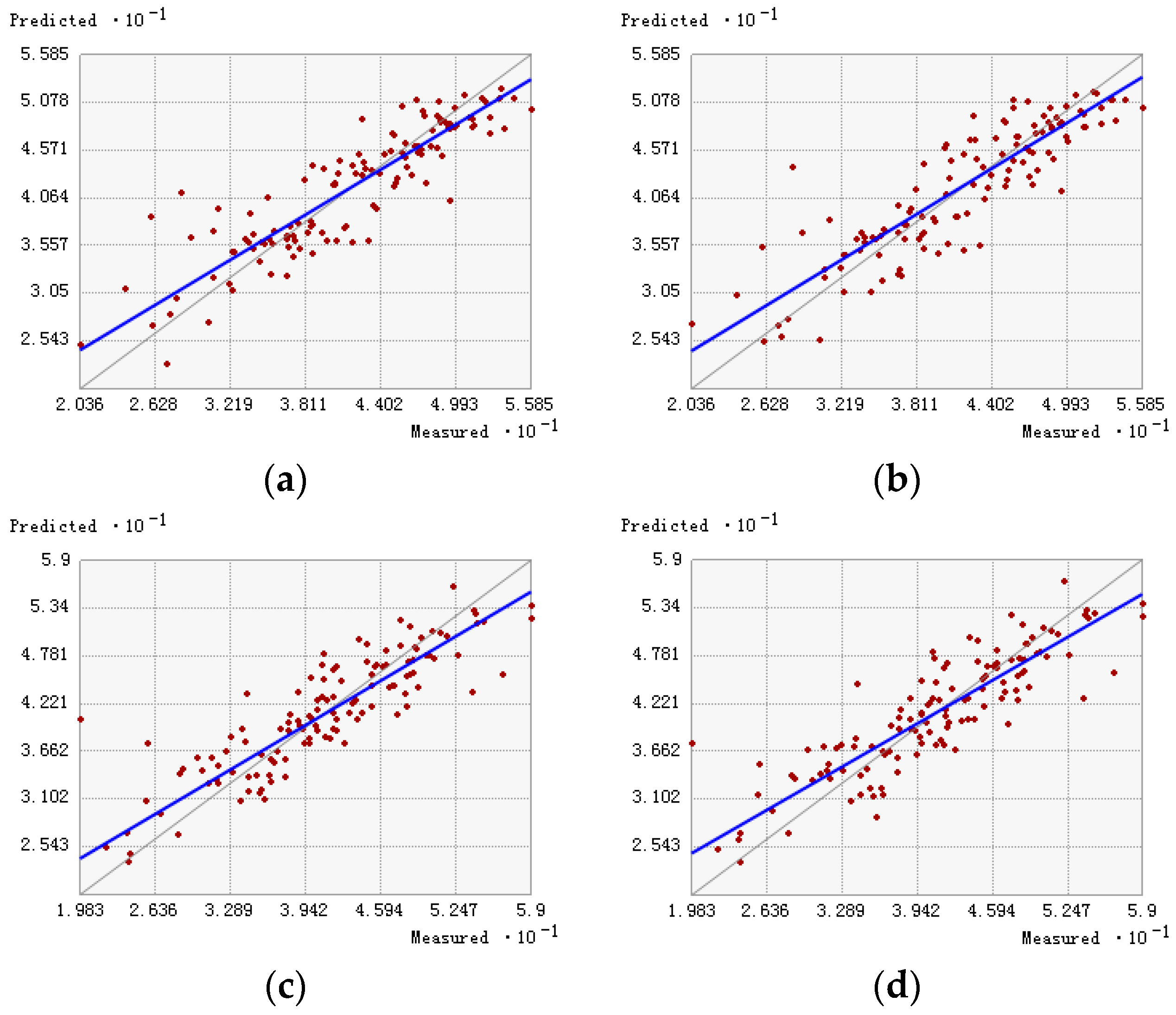
It is important for the simulation precision of LUR based landscape pattern index to get rid of the spatial autocorrelation and detect the normal distribution and trends of PM2.5 concentration in supplementary section (Figures S1–S4). The RMSE of the ordinary kriging for the LUR-based data-mining was 3.512 μg/m3, which of the LUR-based ordinary kriging was 3.571 μg/m3, that of the ordinary kriging was 4.067 μg/m3, and that of the data-mining-based ordinary kriging was 4.055 μg/m3 (Table 5). A smaller RMSE indicates a lower deviation of the predicted values from the measured values. Therefore, the cross-validation results suggested that the simulation accuracy of ordinary kriging for the LUR-based data-mining was better (Figure 2). As found in the pair-wise comparisons, the RMSE was significantly reduced using the LUR model; the accuracy of particle concentration prediction was improved by 0.5 μg/m3. These improvements were attributed to the factors incorporated in the regression model. The factors considered included not only space and distance but also environmental and social factors such as the weather, transportation, population, elevation, and land use. Different influencing factors have different interpretation abilities for the PM2.5 concentration. The use of the LUR model could avoid over-reliance on the spatial and distance factors. Furthermore, the factors incorporated in the model were considered comprehensively, which resulted in predictions that were closer to the actual conditions; hence, the model is based on a more solid scientific foundation.
3.3. Concentration Simulation
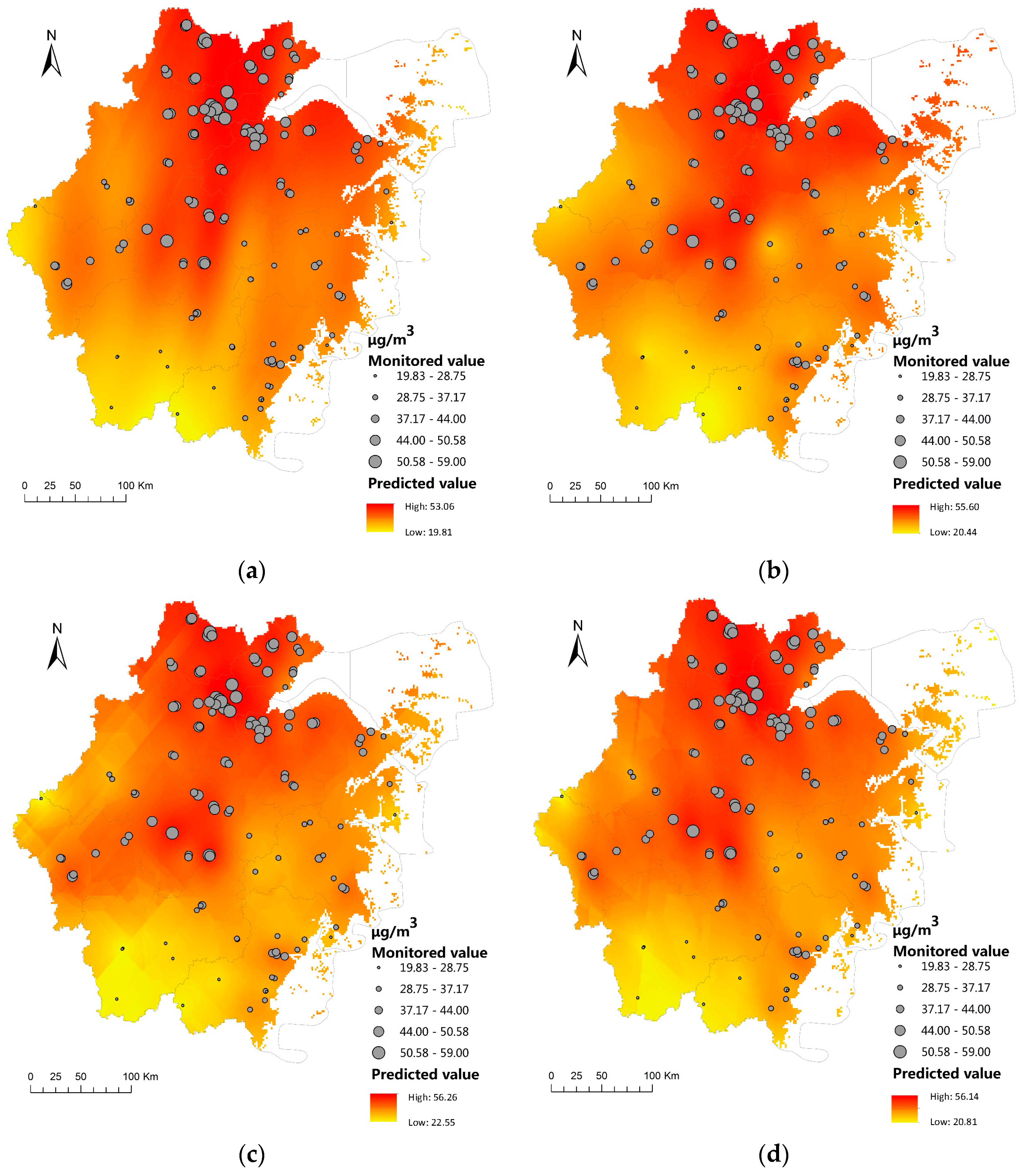
We have compared the prediction accuracy of the different LUR-model application methods in supplementary section, the simulation accuracy was greater when directly applying the land use model to point fitting (Figure S5, Table S1). Compared with the other three methods, ordinary kriging for LUR-based data mining resulted in a prediction range of 19.81–53.06 μg/m3 (Figure 3); for the low-pollution regions, the prediction value was even closer to the monitored range of 19.83–59 μg/m3 (Figure 3). The overall results of the concentration simulation by the four methods were similar. This distribution of prediction value was, to a large extent, consistent with the monitored particle distribution (Figure 3). In particular, the pollution in the northern Zhejiang was severe, but that in the southern region was relatively mild. Among the station of the northern Zhejiang, the PM2.5 concentration at the Zhaohui, Wuqu, and Hemu school station in Hangzhou were detected to be as highest as 59 μg/m3. In addition, the PM2.5 concentration at others in the northern Zhejiang almost more than 40 μg/m3. On the contrary, among the stations of the southern Zhejiang, the PM2.5 concentration were detected to be as low as 40 μg/m3. Although PM2.5 concentration of Qianjiangyuan station in the east was lower than all of sites of the Zhejiang province, the pollution in the east and west of the province were similar, and the degree of severity was between those of the north and south. The heavily polluted regions were mainly located in Huzhou, Jiaxing, Hangzhou, Shaoxing, and the northeast of Jinhua, which were regions with higher levels of urbanization. On the other hand, the landscape in the southern regions was mainly composed of mountains, and the population was more scattered compared with in the north. The southern region also had a higher vegetation coverage, lower emission of pollutants, and higher air humidity. Therefore, the pollutant concentration was lower. Urban planning could directly impact the air quality of a city [40,41]. Without proper guidance and management, rapid urban development will lead to environmental issues and health risks caused by poor air quality. As shown in our study, the air quality can be improved with the following measures: reduce the area of residence within 5000 m of the city center, increase the clustering of lands with the same type of use, suitably increase the area of water bodies within 4000 m of the city center, avoid intensive traffic that triggers the outbreak of pollutant emissions [42,43,44], and allow the dispersion of air pollutants. Although we have proposed some suggestions for improving air quality, there are some shortcomings in our research. Only 150 sites’ data over Zhejiang province was collected to test the model in our study, the representation was limited, and the method was mainly linear, without considered the nonlinear relation between factors. The prediction accuracy of the model still has room for improvement. Although we have a certain understanding of the long-term changes of particulate matter at regional scale, the process of short-term formation and dispersion of particulate matter cannot be caught by the model due to the lack of daily changes.
4. Conclusions
The prediction accuracy of the model with the inclusion of the landscape pattern factors was greater than the model of without the inclusion of the landscape pattern factors. The latitude and 5000_residential_CA were positively correlated to the PM2.5, however, the variables negatively correlated with the PM2.5 were the annual average relative humidity, 5000_CONTAG, and 4000_waters_LPI. Over the lightly polluted region, the predicted value obtained by ordinary kriging for the LUR-based data mining was closest to the monitored value, and the RMSE was the lowest (3.512 μg/m3).
Supplementary Materials
The following are available online at https://www.mdpi.com/2073-4433/9/2/47/s1, Figure S1: Histogram. Figure S2: Normal QQ diagram. Figure S3: Trend analysis: (a) rotational angle of 0°; (b) rotational angle of 90°. Figure S4: Semi-variogram: (a) south-north direction; (b) east-west direction. Figure S5: Predicted pollutant concentration and error distribution resulting from different application mechanisms: (a) applying model to surface fitting; (b) applying model to point fitting. Table S1: Fitting parameters of different application mechanisms.
Acknowledgments
This research was funded by National Natural Science Foundation of China (no. 41471442 and no. 41101421) and Key Science and Technology Innovation Team of Zhejiang Province (No. 2011R50027).
Author Contributions
Jian Chen and Shan Yang conceived and designed the experiments. Shan Yang and Jian Chen performed the experiments and wrote the manuscript. Haitian Wu, Xintao Lin, and Ting Lu participated in the discussions surrounding this study.
Conflicts of Interest
The authors declare no conflict of interest.
References
- Amini, H.; Taghavishahri, S.M.; Henderson, S.B.; Naddafi, K.; Nabizadeh, R.; Yunesian, M. Land use regression models to estimate the annual and seasonal spatial variability of sulfur dioxide and particulate matter in Tehran, Iran. Sci. Total Environ. 2014, 488, 343–353. [Google Scholar] [CrossRef] [PubMed]
- Coker, E.; Ghosh, J.; Jerrett, M.; Gomez-Rubio, V.; Beckerman, B.; Cockburn, M.; Liverani, S.; Su, J.; Li, A.; Kile, M.L. Modeling spatial effects of PM2.5 on term low birth weight in Los Angeles county. Environ. Res. 2015, 142, 354–364. [Google Scholar] [CrossRef] [PubMed]
- Kim, Y.; Guldmann, J.M. Land-use regression panel models of NO2 concentrations in Seoul, Korea. Atmos. Environ. 2015, 107, 364–373. [Google Scholar] [CrossRef]
- Lee, M.; Brauer, M.; Wong, P.; Tang, R.; Tsui, T.H.; Choi, C.; Wei, C.; Lai, P.C.; Tian, L.; Thach, T.Q. Land use regression modelling of air pollution in high density high rise cities: A case study in Hong Kong. Sci. Total Environ. 2017, 592, 306–315. [Google Scholar] [CrossRef] [PubMed]
- Meng, X.; Chen, L.; Cai, J.; Zou, B.; Wu, C.F.; Fu, Q.; Zhang, Y.; Liu, Y.; Kan, H. A land use regression model for estimating the NO2 concentration in Shanghai, China. Environ. Res. 2015, 137, 308–315. [Google Scholar] [CrossRef] [PubMed]
- Meng, X.; Fu, Q.; Ma, Z.; Chen, L.; Zou, B.; Zhang, Y.; Xue, W.; Wang, J.; Wang, D.; Kan, H. Estimating ground-level PM(10) in a Chinese city by combining satellite data, meteorological information and a land use regression model. Environ. Pollut. 2016, 208, 177–184. [Google Scholar] [CrossRef] [PubMed]
- Montagne, D.; Hoek, G.; Nieuwenhuijsen, M.; Lanki, T.; Pennanen, A.; Portella, M.; Meliefste, K.; Eeftens, M.; Ylituomi, T.; Cirach, M. Agreement of land use regression models with personal exposure measurements of particulate matter and nitrogen oxides air pollution. Environ. Sci. Technol. 2013, 47, 8523–8531. [Google Scholar] [CrossRef] [PubMed]
- Sabaliauskas, K.; Jeong, C.H.; Yao, X.; Reali, C.; Sun, T.; Evans, G.J. Development of a land-use regression model for ultrafine particles in Toronto, Canada. Atmos. Environ. 2015, 110, 84–92. [Google Scholar] [CrossRef]
- Shi, Y.; Lau, K.K.; Ng, E. Incorporating wind availability into land use regression modelling of air quality in mountainous high-density urban environment. Environ. Res. 2017, 157, 17–29. [Google Scholar] [CrossRef] [PubMed]
- Gage, E.A.; Cooper, D.J. Relationships between landscape pattern metrics, vertical structure and surface urban heat island formation in a Colorado suburb. Urban Ecosyst. 2017, 20, 1229–1238. [Google Scholar] [CrossRef]
- Jun-Hyun, K.; Gu, D.; Wonmin, S.; Sung-Ho, K.; Hwanyong, K.; Dong-Kun, L. Neighborhood landscape spatial patterns and land surface temperature: An empirical study on single-family residential areas in Austin, Texas. Int. J. Environ. Res. Public Health 2016, 13, 880. [Google Scholar]
- Li, Y.; Liu, G. Characterizing spatiotemporal pattern of land use change and its driving force based on GIS and landscape analysis techniques in Tianjin during 2000–2015. Sustainability 2017, 9, 894. [Google Scholar] [CrossRef]
- Xinliang, X.U.; Cai, H.; Qiao, Z.; Wang, L.; Jin, C.; Yaning, G.E.; Wang, L.; Fengjiao, X.U. Impacts of park landscape structure on thermal environment using quickbird and landsat images. Chin. Geogr. Sci. 2017, 27, 818–826. [Google Scholar]
- Yang, Y.; Li, Z.; Li, P.; Ren, Z.; Gao, H.; Wang, T.; Xu, G.; Yu, K.; Shi, P.; Tang, S. Variations in runoff and sediment in watersheds in loess regions with different geomorphologies and their response to landscape patterns. Environ. Earth Sci. 2017, 76, 517. [Google Scholar] [CrossRef]
- Weber, N.; Haase, D.; Franck, U. Zooming into temperature conditions in the city of Leipzig: How do urban built and green structures influence earth surface temperatures in the city? Sci. Total Environ. 2014, 496, 289–298. [Google Scholar] [CrossRef] [PubMed]
- Bottalico, F.; Travaglini, D.; Chirici, G.; Garfì, V.; Giannetti, F.; Marco, A.D.; Fares, S.; Marchetti, M.; Nocentini, S.; Paoletti, E. A spatially-explicit method to assess the dry deposition of air pollution by urban forests in the city of Florence, Italy. Urban For. Urban Green. 2017, 27, 221–234. [Google Scholar] [CrossRef]
- Liu, H.; Fang, C.; Zhang, X.; Wang, Z.; Bao, C.; Li, F. The effect of natural and anthropogenic factors on haze pollution in Chinese cities: A spatial econometrics approach. J. Clean. Prod. 2017, 165, 323–333. [Google Scholar] [CrossRef]
- Wu, J.; Li, J.; Peng, J.; Li, W.; Xu, G.; Dong, C. Applying land use regression model to estimate spatial variation of PM2.5 in Beijing, China. Environ. Sci. Pollut. Res. Int. 2015, 22, 7045–7061. [Google Scholar] [CrossRef] [PubMed]
- Zou, B.; Luo, Y.; Wan, N.; Zheng, Z.; Sternberg, T.; Liao, Y. Performance comparison of LUR and ok in PM2.5 concentration mapping: A multidimensional perspective. Sci. Rep. 2015, 5, 8698. [Google Scholar] [CrossRef] [PubMed]
- Yang, H.; Chen, W.; Liang, Z. Impact of land use on PM2.5 pollution in a representative city of middle China. Int. J. Environ. Res. Public Health 2017, 14, 462. [Google Scholar] [CrossRef] [PubMed]
- Zhang, A.; Qi, Q.; Jiang, L.; Zhou, F.; Wang, J. Population exposure to PM2.5 in the urban area of Beijing. PLoS ONE 2013, 8, e63486. [Google Scholar] [CrossRef] [PubMed]
- Wilson, J.G.; Zawar-Reza, P. Intraurban-scale dispersion modelling of particulate matter concentrations: Applications for exposure estimates in cohort studies. Atmos. Environ. 2006, 40, 1053–1063. [Google Scholar] [CrossRef]
- Ho, C.C.; Chan, C.C.; Cho, C.W.; Lin, H.I.; Lee, J.H.; Wu, C.F. Land use regression modeling with vertical distribution measurements for fine particulate matter and elements in an urban area. Atmos. Environ. 2015, 104, 256–263. [Google Scholar] [CrossRef]
- Lee, J.H.; Wu, C.F.; Hoek, G.; De, H.K.; Beelen, R.; Brunekreef, B.; Chan, C.C. Lur models for particulate matters in the Taipei metropolis with high densities of roads and strong activities of industry, commerce and construction. Sci. Total Environ. 2015, 514, 178–184. [Google Scholar] [CrossRef] [PubMed]
- Zhai, L.; Zou, B.; Fang, X.; Luo, Y.; Wan, N.; Li, S. Land use regression modeling of PM2.5 concentrations at optimized spatial scales. Atmosphere 2016, 8, 1. [Google Scholar] [CrossRef]
- Mcgarigal, K.; Marks, B.J. FRAGSTATS: Spatial analysis program for quantifying landscape structure. Gen. Tech. Rep. 1995, 351. [Google Scholar] [CrossRef]
- Wu, J.; Xie, W.; Li, W.; Li, J. Effects of urban landscape pattern on PM2.5 pollution-a Beijing case study. PLoS ONE 2015, 10, e0142449. [Google Scholar] [CrossRef] [PubMed] [Green Version]
- Korek, M.; Johansson, C.; Svensson, N.; Lind, T.; Beelen, R.; Hoek, G.; Pershagen, G.; Bellander, T. Can dispersion modeling of air pollution be improved by land-use regression? An example from Stockholm, Sweden. J. Expo Sci. Environ. Epidemiol. 2017, 27, 575–581. [Google Scholar] [CrossRef] [PubMed]
- Lee, J.H.; Wu, C.F.; Hoek, G.; De, H.K.; Beelen, R.; Brunekreef, B.; Chan, C.C. Land use regression models for estimating individual NOX and NO2 exposures in a metropolis with a high density of traffic roads and population. Sci. Total Environ. 2015, 472, 1163–1171. [Google Scholar] [CrossRef] [PubMed]
- Rivera, M.; Basagaña, X.; Aguilera, I.; Agis, D.; Bouso, L.; Foraster, M.; Medina-Ramón, M.; Pey, J.; Künzli, N.; Hoek, G. Spatial distribution of ultrafine particles in urban settings: A land use regression model. Atmos. Environ. 2012, 54, 657–666. [Google Scholar] [CrossRef]
- Grzywna, A.; Kamińska, A.; Bochniak, A. Analysis of spatial variability in the depth of the water table in grassland areas. Rocz. Ochr. Srodowiska 2016, 18, 291–302. [Google Scholar]
- Xiao, Y.; Gu, X.; Yin, S.; Shao, J.; Cui, Y.; Zhang, Q.; Niu, Y. Geostatistical interpolation model selection based on arcgis and spatio-temporal variability analysis of groundwater level in piedmont plains, northwest China. SpringerPlus 2016, 5, 425. [Google Scholar] [CrossRef] [PubMed]
- Jian, C.; Hong, J.; Bin, W.; Zhong, Y.X.; Zi, S.J.; Guo, M.Z.; Shu, Q.Y. Aerosol optical properties from Sun-photometric measurements in Hangzhou, China. Int. J. Remote Sens. 2012, 33, 2451–2461. [Google Scholar]
- Zhang, Y.; Zhang, H.; Deng, J.; Du, W.; Hong, Y.; Xu, L.; Qiu, Y.; Hong, Z.; Wu, X.; Ma, Q. Source regions and transport pathways of PM2.5 at a regional background site in east China. Atmos. Environ. 2017, 167, 202–211. [Google Scholar] [CrossRef]
- Li, X.; Ma, Y.; Wang, Y.; Liu, N.; Hong, Y. Temporal and spatial analyses of particulate matter (PM10 and PM2.5) and its relationship with meteorological parameters over an urban city in northeast China. Atmos. Res. 2017, 198, 185–193. [Google Scholar] [CrossRef]
- Dons, E.; Poppel, M.V.; Kochan, B.; Wets, G.; Panis, L.I. Modeling temporal and spatial variability of traffic-related air pollution: Hourly land use regression models for black carbon. Atmos. Environ. 2013, 74, 237–246. [Google Scholar] [CrossRef]
- Zhao, H.; Che, H.; Zhang, X.; Ma, Y.; Wang, Y.; Wang, H.; Wang, Y. Characteristics of visibility and particulate matter (PM) in an urban area of northeast China. Atmos. Pollut. Res. 2013, 4, 427–434. [Google Scholar] [CrossRef]
- Liu, P.F.; Zhao, C.S.; Bel, T.G.; Hallbauer, E.; Nowak, A.; Ran, L.; Xu, W.Y.; Deng, Z.Z.; Ma, N.; Mildenberger, K. Hygroscopic properties of aerosol particles at high relative humidity and their diurnal variations in the north China plain. Atmos. Chem. Phys. 2011, 11, 3479–3494. [Google Scholar] [CrossRef]
- Liang, L.U.; Luo, G.; Zhao, S.T. Land use and land cover change on slope in Qiandongnan prefecture of southwest China. J. Mt. Sci. 2014, 11, 762–773. [Google Scholar]
- Eliasson, I. The use of climate knowledge in urban planning. Landsc. Urban Plan. 2000, 48, 31–44. [Google Scholar] [CrossRef]
- Marquez, L.O.; Smith, N.C. A framework for linking urban form and air quality. Environ. Model. Softw. 1999, 14, 541–548. [Google Scholar] [CrossRef]
- Cheng, S.; Lang, J.; Zhou, Y.; Han, L.; Wang, G.; Chen, D. A new monitoring-simulation-source apportionment approach for investigating the vehicular emission contribution to the PM2.5 pollution in Beijing, China. Atmos. Environ. 2013, 79, 308–316. [Google Scholar] [CrossRef]
- Song, Y.; Xie, Z.S.; Zeng, L.; Zheng, M.; Salmon, L.G.; Shao, M.; Slanina, S. Source apportionment of PM2.5 in Beijing by positive matrix factorization. Atmos. Environ. 2006, 40, 1526–1537. [Google Scholar] [CrossRef]
- Sun, Y.; Zhuang, G.; Wang, Y.; Han, L.; Guo, J.; Dan, M.; Zhang, W.; Wang, Z.; Hao, Z. The air-borne particulate pollution in Beijing—Concentration, composition, distribution and sources. Atmos. Environ. 2004, 38, 5991–6004. [Google Scholar] [CrossRef]
Figure 1.
Distribution and elevation of the national air quality monitoring stations in Zhejiang province.
Figure 1.
Distribution and elevation of the national air quality monitoring stations in Zhejiang province.
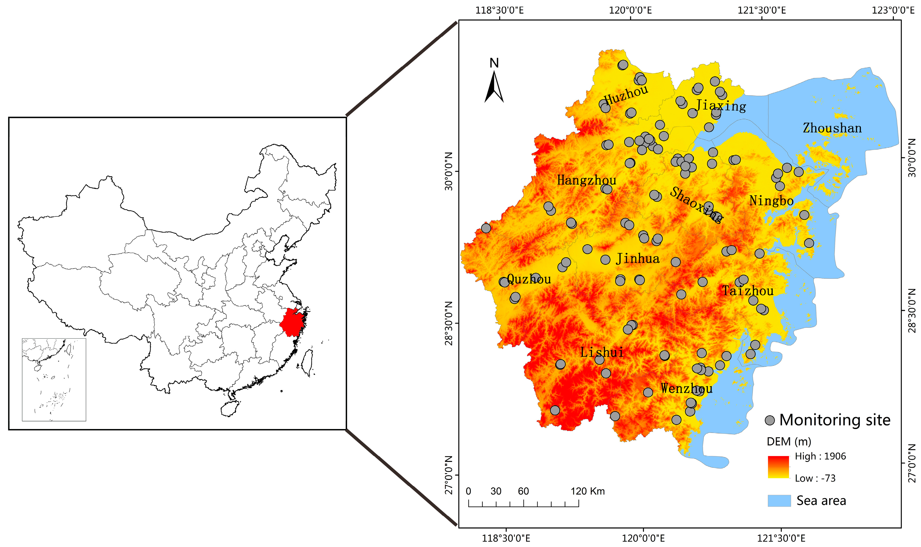
Figure 2.
Cross-validation for the four different simulation methods: (a) ordinary kriging for LUR-based data mining; (b) LUR-based ordinary kriging; (c) ordinary kriging; (d) data-mining-based ordinary kriging.
Figure 2.
Cross-validation for the four different simulation methods: (a) ordinary kriging for LUR-based data mining; (b) LUR-based ordinary kriging; (c) ordinary kriging; (d) data-mining-based ordinary kriging.

Figure 3.
Pollutant concentration simulation by the four different methods: (a) ordinary kriging for LUR-based data mining; (b) LUR-based ordinary kriging; (c) ordinary kriging; (d) data-mining-based ordinary kriging.
Figure 3.
Pollutant concentration simulation by the four different methods: (a) ordinary kriging for LUR-based data mining; (b) LUR-based ordinary kriging; (c) ordinary kriging; (d) data-mining-based ordinary kriging.


Table 1.
Landscape pattern index of different distance buffers.
| Landscape Pattern Index Category | Description (Within Each Buffer) | Buffer Distance (m) | Land Use Types | Variables Names (Example) |
|---|---|---|---|---|
| Class area (CA) | Total area of land cover types | 100, 300, 500, 800, 1000, 2000, 3000, 4000, 5000 | woodland, residence, industrial, commercial, urban greenery, transportation, agricultural, bare land, waters, roads | buffer-distance_land-use-type_landscape-pattern indexes (100_woodland_CA 300_residence_PLAND 500_industrial_LPI 800_commercial_ED 1000_urban greenery_PD 2000_transportation_CONTAG 3000_agricultural_SHDI 4000_bare land_SHEI) |
| Percent of landscape (PLAND) | The percentage of area of different patch types | |||
| Largest patch index (LPI) | Largest area of different patch types | |||
| Edge density (ED) | The length of the unit area of different patch type | |||
| Patch density (PD) | The number of different patch type of unit area | |||
| Contagion index (CONTAG) | The degree of clustering or trend of extension of different patch type | |||
| Shannon’s diversity index (SHDI) | The diversity of patch type | |||
| Shannon’s evenness index (SHEI) | The degree of inhomogeneity of different patch |
Table 2.
List of variables of modeling.
| Variables | Variables | Variables |
|---|---|---|
| Latitude | 5000_woodland_CA | 5000_residential_CA |
| DEM | 500_woodland_CA | 1000_residential_CA |
| Population density | 300_woodland_CA | 800_residential_CA |
| Wind speed | 100_woodland_CA | 500_residential_CA |
| Pressure | 5000_woodland_PLAND | 300_residential_CA |
| Relative humidity | 500_woodland_PLAND | 5000_residential_PLAND |
| Temperature | 300_woodland_PLAND | 1000_residential_PLAND |
| Rainfall | 100_woodland_PLAND | 800_residential_PLAND |
| 5000_CONTAG | 1000_woodland_PD | 500_residential_PLAND |
| 5000_SHDI | 800_woodland_PD | 300_residential_PLAND |
| 5000_SHEI | 500_woodland_PD | 800_residential_PD |
| 4000_waters_LPI | 100_woodland_PD | 5000_residential_LPI |
| 5000_transportation_LPI | 5000_woodland_LPI | 800_residential_LPI |
| 5000_roads_CA | 100_woodland_LPI | 1000_residential_LPI |
| 500_roads_CA | 500_woodland_LPI | 5000_commercial_CA |
| 5000_roads_PLAND | 300_woodland_LPI | 5000_commercial_PLAND |
| 500_roads_PLAND | 2000_woodland_ED | 300_commercial_PD |
| 5000_roads_PD | 100_woodland_ED | 2000_commercial_PD |
| 4000_roads_LPI | 5000_agricultural_CA | 5000_commercial_PD |
| 2000_roads_LPI | 5000_agricultural_PLAND | 5000_commercial_ED |
| 800_roads_LPI | 1000_agricultural_PD | 5000_commercial_LPI |
| 5000_roads_ED | 5000_residential_ED |
DEM: Digital Elevation Model.
Table 3.
Parameters of the multiple regression model with the inclusion of landscape pattern factors.
Table 3.
Parameters of the multiple regression model with the inclusion of landscape pattern factors.
| Model | Unstandardized Coefficients | Standardized Coefficients | t | Significance | |
|---|---|---|---|---|---|
| B | Std. Error | Beta | |||
| Constant | 17.802 | 19.266 | 0.924 | 0.357 | |
| Latitude | 4.202 | 0.357 | 0.498 | 11.775 | 0.000 |
| Relative humidity | −1.257 | 0.215 | −0.265 | −5.854 | 0.000 |
| 5000_residential_CA | 0.003 | 0 | 0.317 | 6.383 | 0.000 |
| 5000_CONTAG | −0.155 | 0.038 | −0.183 | −4.068 | 0.000 |
| 4000_waters_LPI | −0.111 | 0.039 | −0.114 | −2.857 | 0.005 |
| Adjust R square | 0.805 | F | 103.212 | Sig. | 0.000 |
| RMSE | 3.420 | ||||
RMSE: Root-Mean-Square Error.
Table 4.
Parameters of the multiple regression model prior to the inclusion of landscape pattern factors.
Table 4.
Parameters of the multiple regression model prior to the inclusion of landscape pattern factors.
| Model | Unstandardized Coefficients | Standardized Coefficients | t | Significance | |
|---|---|---|---|---|---|
| B | Std. Error | Beta | |||
| Constant | 38.062 | 22.921 | 1.661 | 0.099 | |
| Latitude | 4.917 | 0.448 | 0.583 | 10.975 | 0.000 |
| Relative humidity | −1.853 | 0.248 | −0.391 | −7.468 | 0.000 |
| DEM | −0.014 | 0.006 | −0.127 | −2.244 | 0.027 |
| Adjust R square | 0.681 | F | 73.342 | Sig. | 0.000 |
| RMSE | 4.680 | ||||
DEM: Digital Elevation Model; RMSE: Root-Mean-Square Error.
Table 5.
Cross-validation parameters for the four different simulation methods.
| Cross-Validation Parameters | Ordinary Kriging for LUR-Based Data Mining | LUR-Based Ordinary Kriging | Ordinary Kriging | Data-Mining-Based Ordinary Kriging |
|---|---|---|---|---|
| RMSE | 3.512 | 3.571 | 4.067 | 4.055 |
| Regression function | 8.009 + 0.809x | 7.715 + 0.819x | 8.252 + 0.798x | 9.409 + 0.772x |
© 2018 by the authors. Licensee MDPI, Basel, Switzerland. This article is an open access article distributed under the terms and conditions of the Creative Commons Attribution (CC BY) license (http://creativecommons.org/licenses/by/4.0/).
Share and Cite
MDPI and ACS Style
Yang, S.; Wu, H.; Chen, J.; Lin, X.; Lu, T. Optimization of PM2.5 Estimation Using Landscape Pattern Information and Land Use Regression Model in Zhejiang, China. Atmosphere 2018, 9, 47. https://doi.org/10.3390/atmos9020047
AMA Style
Yang S, Wu H, Chen J, Lin X, Lu T. Optimization of PM2.5 Estimation Using Landscape Pattern Information and Land Use Regression Model in Zhejiang, China. Atmosphere. 2018; 9(2):47. https://doi.org/10.3390/atmos9020047
Chicago/Turabian StyleYang, Shan, Haitian Wu, Jian Chen, Xintao Lin, and Ting Lu. 2018. "Optimization of PM2.5 Estimation Using Landscape Pattern Information and Land Use Regression Model in Zhejiang, China" Atmosphere 9, no. 2: 47. https://doi.org/10.3390/atmos9020047
Note that from the first issue of 2016, this journal uses article numbers instead of page numbers. See further details here.